High-Density UAV-LiDAR in an Integrated Crop-Livestock-Forest System: Sampling Forest Inventory or Forest Inventory Based on Individual Tree Detection (ITD)

Abstract

Lidar point clouds have been frequently used in forest inventories. The higher point density has provided better representation of trees in forest plantations. So we developed a new approach to fill this gap in the integrated crop-livestock-forest system, the sampling forest inventory, which uses the principles of individual tree detection applied under different plot arrangements. We use a UAV-lidar system (GatorEye) to scan an integrated crop-livestock-forest system with Eucalyptus benthamii seed forest plantations. On the high density UAV-lidar point cloud (>1400 pts. m²), we perform a comparison of two forest inventory approaches: Sampling Forest Inventory (SFI) with circular (1380 m² and 2300 m²) and linear (15 trees and 25 trees) plots and Individual Tree Detection (ITD). The parametric population values came from the approach with measurements taken in the field, called forest inventory (FI). Basal area and volume estimates were performed considering the field heights and the heights measured in the LiDAR point clouds. We performed a comparison of the variables number of trees, basal area, and volume per hectare. The variables by scenarios were submitted to analysis of variance to verify if the averages are considered different or equivalent. The RMSE (%) were calculated to explain the deviation between the measured volume (filed) and estimated volume (LiDAR) values of these variables. Additionally, we calculated rRMSE, Standard error, AIC, R², Bias, and residual charts. The basal area values ranged from 7.40 m² ha⁻¹ (C1380) to 8.14 m² ha⁻¹ 281 (C2300), about −5.9% less than the real value (8.65 m² ha⁻¹). The C2300 scenario was the only one whose confidence interval (CI) limits included the basal area real. For the total stand volume, the ITD scenario was the one that presented the closer values (689.29 m³) to the real total value (683.88 m³) with the real value positioned in the CI. Our findings indicate that for the stand conditions under study, the SFI approach (C2300) that considers an area of 2300 m² is adequate to generate estimates at the same level as the ITD approach. Thus, our study should be able to assist in the selection of an optimal plot size to generate estimates with minimized errors and gain in processing time.

1. Introduction

Forest plantation area is constantly increasing across the globe, and the goods and services provided by these forests are becoming tremendously diverse [1]. In this context, Brazilian forest plantations stand out with a prominent position, in which more than 10 million ha supply industries of pulp and paper, fuelwood, and solid wood products [2,3]. Brazilian forest industries demand millions of cubic meters of wood annually. Thus, fast and reliable information regarding stand structure and wood availability is crucial to ensure industrial demand [4].

Eucalypt stands are the most important source of short fiber pulp, fuelwood, and charcoal due to their fast growth and wood properties [5]. Usually, fast-growing eucalypt plantations are grown in monoculture. There is, however, a recent increase in crop-livestock-forest system area [6]. Eucalyptus trees established in crop-live-stock-forest systems are usually planted in rows, presenting lower stand density and diverse canopy structures. Consequently, defining sampling strategies for these trees becomes a challenging endeavor, resulting in a lack of literature-review based recommendations [7]. Forest inventories are considered an essential source of quantitative and qualitative information for the management of forest resources [8]. However, the traditional methods are considered complex and laborious activities, and remote sensing methods have emerged as auxiliary tools for attaining fast and reliable data [9]. In [10], the authors highlighted the main technologies for remote sensing-assisted forest inventories, and Light Detection and Ranging (LiDAR) was listed as a major player.

In particular, airborne LiDAR has emerged as one of the most promising remote sensing technologies for estimating forest attributes due to its ability to reconstruct the detailed 3D structure of the entire forest landscape using airplane-mounted high-frequency laser scanners. In this way, they might potentially overtake or assist the traditional in-situ forest inventory since they can collect more information in high resolution and accuracy in a relatively short period [11,12]. So far, this technology has been used to predict forest structural parameters, such as forest height [13,14], canopy density [15], species diversity [16], above-ground biomass [17] and even individual tree attributes [18].

Even though LiDAR can acquire horizontal and vertical information on forest structure at high spatial resolutions and vertical accuracies, it was mainly applied over small- and moderate-scale applications, owing to the financial constraints [19]. Besides that, since it is usually acquired by aircraft, the achievable density was typically between 1 to 10 points/m², depending on flight altitude and scanner configuration. Recently, LiDAR sensors have been mounted on UAVs (Unmanned Aerial Vehicle) to combine the advantages of LiDAR and UAV technology. UAV systems represent a low-cost, agile, and autonomous opportunity, making them an alternative platform to satellites and aircraft for forest inventories [20,21,22]. Furthermore, by flying at a significantly lower altitude than traditional aircraft, UAV’s systems offer the possibility of generating high-density clouds.

Forest attributes can be predicted by two main approaches using LiDAR data [23]. One of these methods is referred to as the area-based approach (ABA), which uses statistics describing the vertical distribution of LiDAR returns to estimate common forest inventory variables across a regular grid of pixels [24]. In addition, the analysis is performed in fixed sampling areas [11,25]. In the area approach the forest inventory is conducted by applying sampling techniques (SFI—sampling forest inventory). The other approach is individual tree detection (ITD), which refers to the division of the point cloud into individual trees, using a segmentation algorithm [26]. These approaches have been used primarily on forest stands with regular spacing and homogeneous crown structures, such as those composed of conifer species [27]. Recent studies, however, have investigated the performance of UAV-LiDAR data to perform the ITD approach for eucalypt stands [24]. Although comparative analyses between ABA and ITD have been developed, most have low-density LiDAR data as input. UAV-LiDAR sensors have provided high-density point clouds that can greatly contribute to improving the estimates of individual trees [28] Additionally, few studies have been concerned with proposing methodological approaches, even in traditional forest inventories, for integrated crop-livestock-forest systems.

Our main motivation for the study is to provide in the integrated crop-livestock-forest system producers with a faster and cheaper alternative for conducting forest inventories. However, we need to be sure that the technology works accurately. This question has not yet been properly investigated for in the integrated crop-livestock-forest system.

Through our study, we explore the following questions: can we improve/alter the traditional approach of forest inventory with sampling techniques in plots (in this study referred to as Forest Inventory by Sampling—SFI) to techniques that use more remote sensing technology, in this case considering point clouds of LiDAR data to measure individual tree variables as samples (in this study referred to as Individual Tree Detection—ITD) that would be multiplied by the number of trees obtained by parametric counting in point clouds? Could this change in approach provide better accuracy in the estimates generated? To answer these questions, several variables such as the number of trees, basal area, and stand volume were evaluated. To support our findings, we count on a complete census at the stand. To the best of our knowledge, this study is the first initiative to address the performance of both SFI and ITD approaches for eucalypt trees established in a crop-livestock-forest system.

2. Materials and Methods

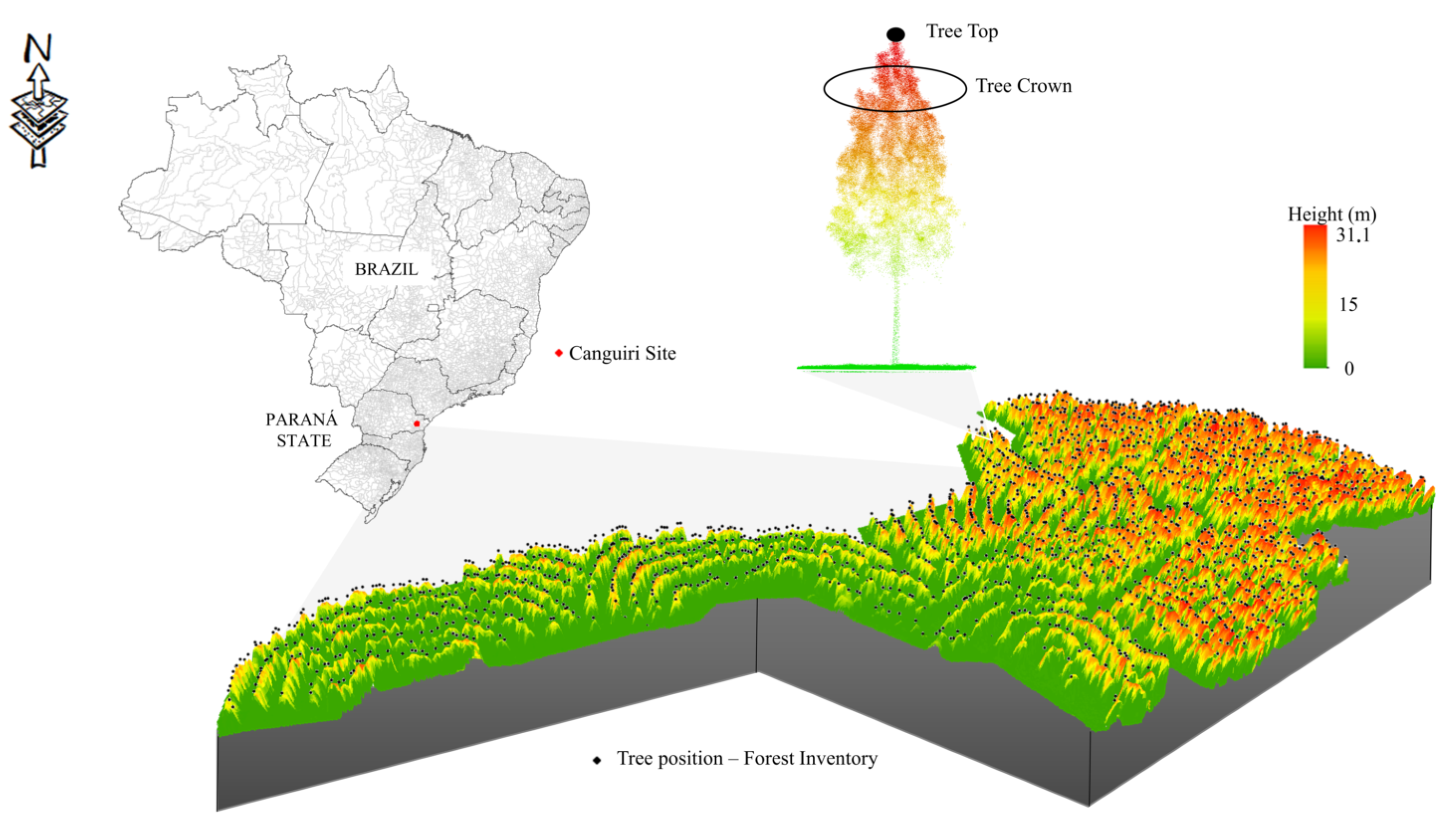
2.1. Study Area Description

This study used data from eucalypt stands (Eucalyptus benthamii Maiden et Cambage) established in a crop-livestock-forest system—iCLF (Figure 1) of age six years. These eucalypt stands are located in a 15.79 ha research trial (at the Canguiri Site) located in the municipality of Pinhais in the State of Paraná, southern Brazil (25°22′38′′ S, 49°09′05′′ W). The stands were established in Haplic Cambisols, following the Brazilian System of Soil Classification [29]. These soils correspond to Inceptisols in Soil Taxonomy—NRCS [30]. The municipality of Pinhais is encompassed by a humid subtropical climate (without dry season and with temperate summer)—Cfb, according to Köppen Classification [31]. The average elevation is 920 m above sea level, and annual rainfall is around 1550 mm. The average initial spacing was 2 m × 14 m, totaling 357 trees ha⁻¹ [32].

2.2. UAV-LiDAR Data

The UAV-LiDAR data were obtained in September 2019 with the GatorEye system [28,33], this equipment presents the following components: flight platform, mission planning, base station, and computational core [34]. The University of Florida developed the GatorEye system with the collaboration of Phoenix LiDAR Systems and Headwall Photonics.

The flight platform is a DJI Matrice 600 Pro hexacopter with a 5 km telemetry and a set of ten batteries. The Universal Ground Control Station (UGCS) software was used for mission planning control. Meanwhile, the base station used the online Trimble CenterPoint RTX post-processing platform, providing <2 cm 3D uncertainty with a 2-h collection period (and <0.25 cm in 4+ h collection). The computational core system is based on a Phoenix Scout + core with a Novatel STIM 300 IMU tactical grade and differential GNSS system. It includes a Velodyne VLP-32c LiDAR sensor, a Nano VNIR Hyperspectral Headwall sensor (640 pixels × 270 spectral bands in a 100-hertz line scan approach), a 25 MP visual sensor, and a radiometric thermal sensor. Velodyne ultra-puck sensor VLP-32c LiDAR sensor uses 32 infra-red (IR) lasers paired with IR detectors to measure objects’ distances.

The mission plan also flew slow (8 m s⁻¹) and low (45 m above ground level), and with flight lines tightly spaced (15 m apart), resulting in a sidelap cross-swath coverage of 93%. The final point density was 1500–2500 points m⁻². Data collection and point cloud specifications are further described in [33]. LiDAR flight lines were processed to standard products using the GatorEye Multi-scalar Post-Processing workflow, using the software Lastools [35] and “lidR” R package [36], which automatically merges flight lines, removes noise, and then generates rasters products and cleaned point clouds [28].

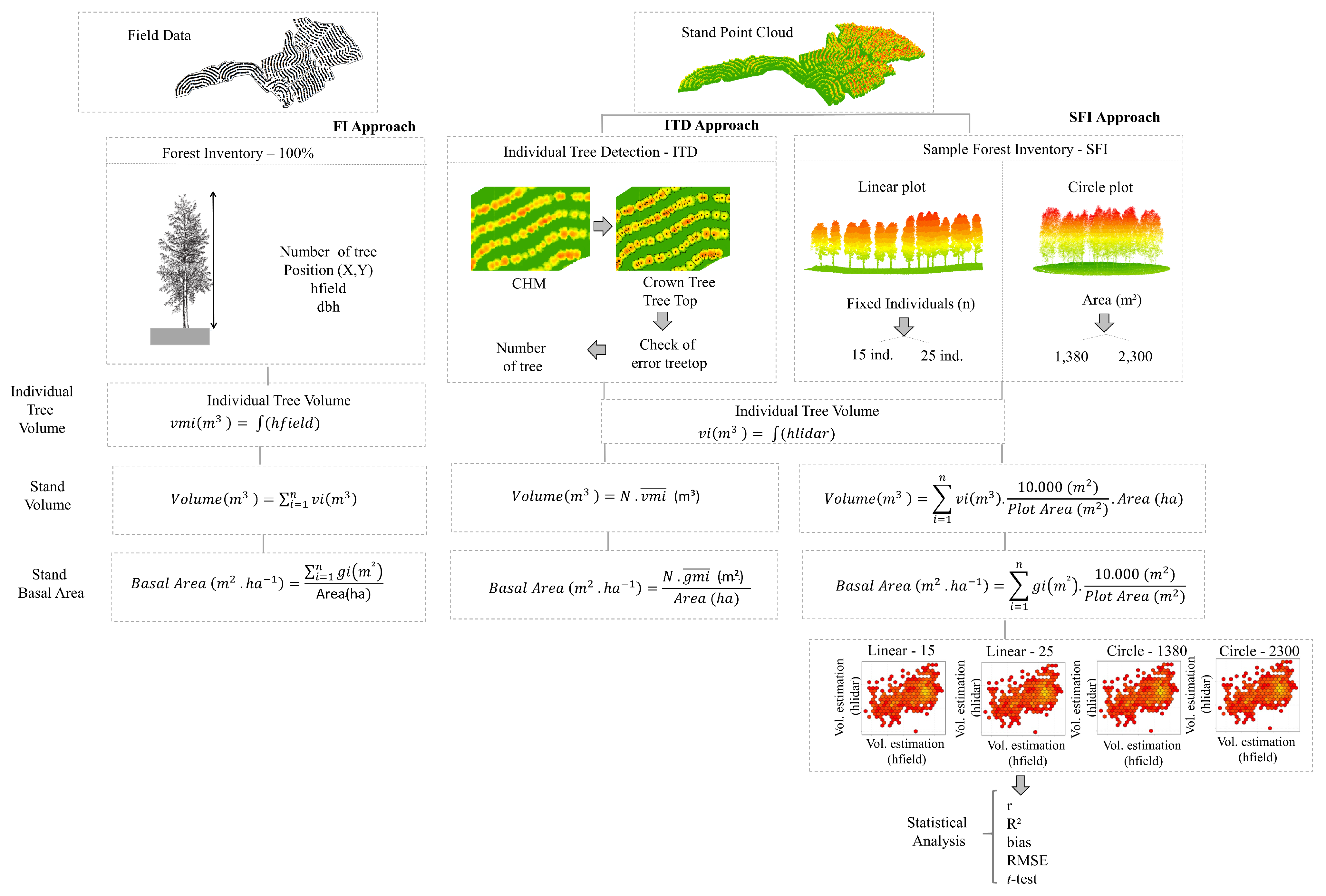
2.3. Methodological Approach

Three methodological approaches were developed (Figure 2). The first approach focused on forest inventory based on a complete census data from the field, called FI. This approach was considered as the baseline in the comparison of the generated estimates. The second and third approaches were derived from UAV-LiDAR data. The second approach was called Individual Tree Detection (ITD) where the individual volume was calculated as a function of the total tree height obtained from the point cloud (hLiDAR) variable and the number of trees was obtained by counting the trees on the point cloud. The third approach is called Sampling Forest Inventory (SFI), sample plots of different sizes and shapes were simulated and the individual tree volume was calculated as a function of the hLiDAR variable. Extrapolation to the hectare was performed using the sum of the plot volumes.

2.4. Forest Inventory Based on a Complete Census (FI)

The eucalyptus stands were assessed by forest inventory based on a complete census, in which all trees were measured with respect to their diameter at 1.3 m above the ground (dbh) and total height (ht). Tree dbh and ht were always measured using a diameter tape and a Haglöf Vertex IV hypsometer. Additionally, all trees (N = 1869) had their geographical position recorded using a GPS (Garmin model 62CSX) to build a geographic information system.

Thereafter, 30 trees were selected for volume destructive sampling. Hence, all 30 trees were felled, bucked and scaled, and measurements of stem were taken in relative heights of the total height (5%, 15%, 25%, 35%, 45%, 55%, 65%, 75%, 85%, and 95%). The individual tree volume (v) was obtained by computing the volume of each section by the Smalian formula (which involves the average cross-sectional area of the large and small ends times the log length). The individual tree volume (v) was assessed by three approaches. First, we used the destructive sampling dataset (with 30 trees) to fit a regression equation based on field-based (Forest inventory based on a complete census—FI) tree heights (hfield) as in Equation (1). After investigating the relationship between the variables, it was observed that the linear regression with the variables transformed to “ln” natural logarithm best expressed the relationship. For this reason, it was applied to all estimates in the paper (Equations (1)–(3), (12) and (13)).

$$ln\left(\widehat{v}\right)=\beta 0+\beta 1ln{\left(hfield\right)}^2.$$

(1)

In the equation, $\widehat{v}$ is the predicted total tree volume (in m³); h is the total tree height field-based data; $\beta$0 = −9.88328; $\beta$1 = 2.955584.

Individual Tree Detection (ITD)

LiDAR point-cloud was used for generating the normalized “.las” file, in addition to the Digital Terrain Model (DTM) and the Canopy Height Model (CHM) (using function grid-canopy at 0.5 m resolution). Thereafter, each tree’s position was determined by the Local Maximum Filter (LMF) within a 3 × 3 window using the find–trees function in the LidR package in R [36,37]. The find–trees function uses the CHM and the normalized LiDAR point-cloud (.las) as inputs for individual tree detection. The dalponte2016 algorithm was used to delineate and segment each tree and assign a new identification attribute (treeID). Finally, the crown of each tree was delineated using the delineate-crowns function, while LiDAR-derived total tree height (hLiDAR) was derived using tree-metrics function. In this approach the transverse area (gi) and the individual volume (vi) were estimated based on LiDAR-derived tree heights (hLiDAR) Equations (2) and (3).

$$ln(\widehat{gi})=\beta 0+\beta 1ln{\left(hLiDAR\right)}^2.$$

(2)

In the equation, $\widehat{gi}$ is the predicted transverse area (in m²); hLiDAR = total tree height UAV-LiDAR data; $\beta$0 = −6.61803; $\beta$1 = 1.34301.

$$ln(\widehat{vi})=\beta 0+\beta 1ln{\left(hLiDAR\right)}^2.$$

(3)

In the equation, $\widehat{vi}$ is the predicted total tree volume (in m³); hLiDAR = total tree height UAV-LiDAR data; $\beta$0 = −9.88328; $\beta$1 = 2.955584.

Each segmented tree was incorporated and exported in a shapefile. This shapefile was visually examined in ArcMap to check detection accuracy by overlaying each tree crown with CHM raster. Subsequently, all segmented and identified trees were counted, resulting in the approximated population density parameter (total number of trees—NITD-based). Hence, the mean individual tree volume (predicted through Equation (3) was used to compute stand volume by multiplying by the number of segmented trees to get the stand volume Equation (4). A similar approach was applied to obtain the basal area of the stand Equation (5).

$$Standvolume\left(V{\mathrm{m}}^3\right)=\sum _{i=1}^n\left(n_i\right)·\underline{v}.$$

(4)

$$BasalArea\left({\mathrm{m}}^2{\mathrm{ha}}^{-1}\right)=\frac{N·\widehat{gi}\left({\mathrm{m}}^2\right)}{Area\left(\mathrm{ha}\right)}.$$

(5)

In the equation, V is the stand volume (in m³); $n_i$ is the ith segmented tree; $\underline{v}$ is the mean individual tree volume (in m³).

The ITD approach for variable N is based on a complete census; this variable faithfully represents the population. Therefore, the calculation of the confidence interval was based on the variability that existed in the volume of individual trees. In this case, since an vmi was used for the estimation in the field, there occurred some variability.

The total estimate was obtained by multiplying the number of trees (forest inventory based on a complete census) by the average of individual tree volume Equation (6). Equation (7) was used to calculate the variance ($s_{vi}^2$), and the standard deviation ($s_{vi}$) was calculated by the square root of the variance. The standard error ($S\overline{vi}$) of sampling was calculated with Equation (8). The absolute error ($Ea$) of the forest inventory was obtained with Equation (9). Finally, the confidence interval ($CI$) for the population was calculated based on Equations (10) (lower limit) and (11) (upper limit).

$$TotalEstimation=N·\overline{vmi}.$$

(6)

$$s_{vi}^2=\frac{{\sum }_{i=1}^n{(vi-\overline{vmi})}^2}{n-1}.$$

(7)

$$S\overline{vi}=\pm \frac{s_{vi}}{\sqrt{n}}.$$

(8)

$$Ea=\pm t·S\overline{vi}.$$

(9)

$$C{I}_{lowerlimit}=N·[\overline{vmi}-t·S\overline{vi}].$$

(10)

$$C{I}_{upperlimit}=N·[\overline{vmi}+t·S\overline{vi}].$$

(11)

where: N = total number of trees; vmi = average of individual tree volume; n = number of trees; vi = individual tree volume i; n = number of plots; t = t-Student.

2.5. Sampling Forest Inventory (SFI)

A total of four different sampling strategies were designed and evaluated, being two scenarios based on circular plots (fixed area) and two with linear plots (fixed number of trees). The area of the circular plots were 1380 m² (C1380 with 35 sample units) and 2300 m² (C2300 with 35 sample units), while the linear plots contained 15 (L15) and 25 trees (L25) along planting rows. The central point of each plot was randomly allocated within the LiDAR point-cloud. In this approach the transverse area (gi) and the individual volume (vi) were estimated based on LiDAR-derived tree heights (hLiDAR) Equations (12) and (13).

$$ln(\widehat{gi})=\beta 0+\beta 1ln{\left(hLiDAR\right)}^2.$$

(12)

In the equation, $\widehat{gi}$ is the predicted transverse area (in m²); hLiDAR total tree height UAV-LiDAR data; $\beta$0 = −6.61803; $\beta$1 = 1.34301.

$$ln(\widehat{vi})=\beta 0+\beta 1ln{\left(hLiDAR\right)}^2.$$

(13)

In the equation, $\widehat{vi}$ is the predicted total tree volume (in m³); hLiDAR = total tree height UAV-LiDAR data; $\beta$0 = −9.88328; $\beta$1 = 2.955584. All trees within the plot had their volume estimated by Equation (3) and the volume of the plot resulted from the sum of these $(V_{plot}{\mathrm{m}}_3·\mathrm{plot}{\mathrm{area}}^{-1})$. Finally, it was multiplied by the area of the plot and the total volume was obtained.

The plot-level volume was computed for each SFI scenario. Measures of dispersion (variance and standard deviation) and central tendency (mean) were assessed and summarized. Subsequently, stand volume was determined by extrapolating the mean plot-level volume to the total area (Equation (14)). In addition, the variance (Equation (15)), standard error of the mean (Equation (16)), sampling error (Equation (17)), and the confidence intervals (Equations (18) and (19)) were determined following the simple random sampling (SRS) protocol [38,39].

$$TotalEstimation=Area·\overline{x}.$$

(14)

$$s_x^2=\frac{{\sum }_{i=1}^n{(X-\overline{x})}^2}{n-1}.$$

(15)

$$s\overline{x}=\pm \frac{s_x}{\sqrt{n}}.$$

(16)

$$Ea=\pm t·S\overline{x}.$$

(17)

$$C{I}_{lowerlimit}=Area·[\overline{x}-t.S\overline{x}].$$

(18)

$$C{I}_{upperlimit}=Area·[\overline{x}+t.S\overline{x}].$$

(19)

where: Area = stand area (hectare); $\overline{x}$ = average of variable per hectare; X = variable per hectare of plot i; n = number of plots; vi = individual tree volume i; n = number of trees; t—t-Student.

2.6. Statistical Analysis and Comparisons

The variables by scenarios were submitted to analysis of variance to verify if the averages are considered different or equivalent. A completely randomized design (CRD) was used, testing the following null hypothesis: $H_0$: it is a statement that there is no difference between a sample mean or proportion and a population mean or proportion. In other words, the difference is equal to 0. $H_1$: it is a claim about the population that is contradictory to $H_0$ and what we conclude when we reject $H_0$. Homogeneity of variance and normality were also tested.

The root mean square absolute and relative root mean square errors (RMSE) (%) were calculated to explain the deviation between the measured volume (estimated from hfield) and estimated volume (estimated from hLiDAR) values of these variables. Additionally, we calculated Relative Root Mean Square Error (rRMSE), Standard error, Akaike information criterion (AIC), Coefficient of Determination (R²), Bias, and residual charts [40,41,42,43]. Pearson’s correlation coefficient (r) was used to quantify the correlation between the observed and the predicted values for each predictive model [44]. An r value of 1 indicates a perfect correlation between predicted and observed values. A test of difference of means was performed for volume, basal area, and number of trees results from the different approaches in accordance with (Figure 3).

3. Results

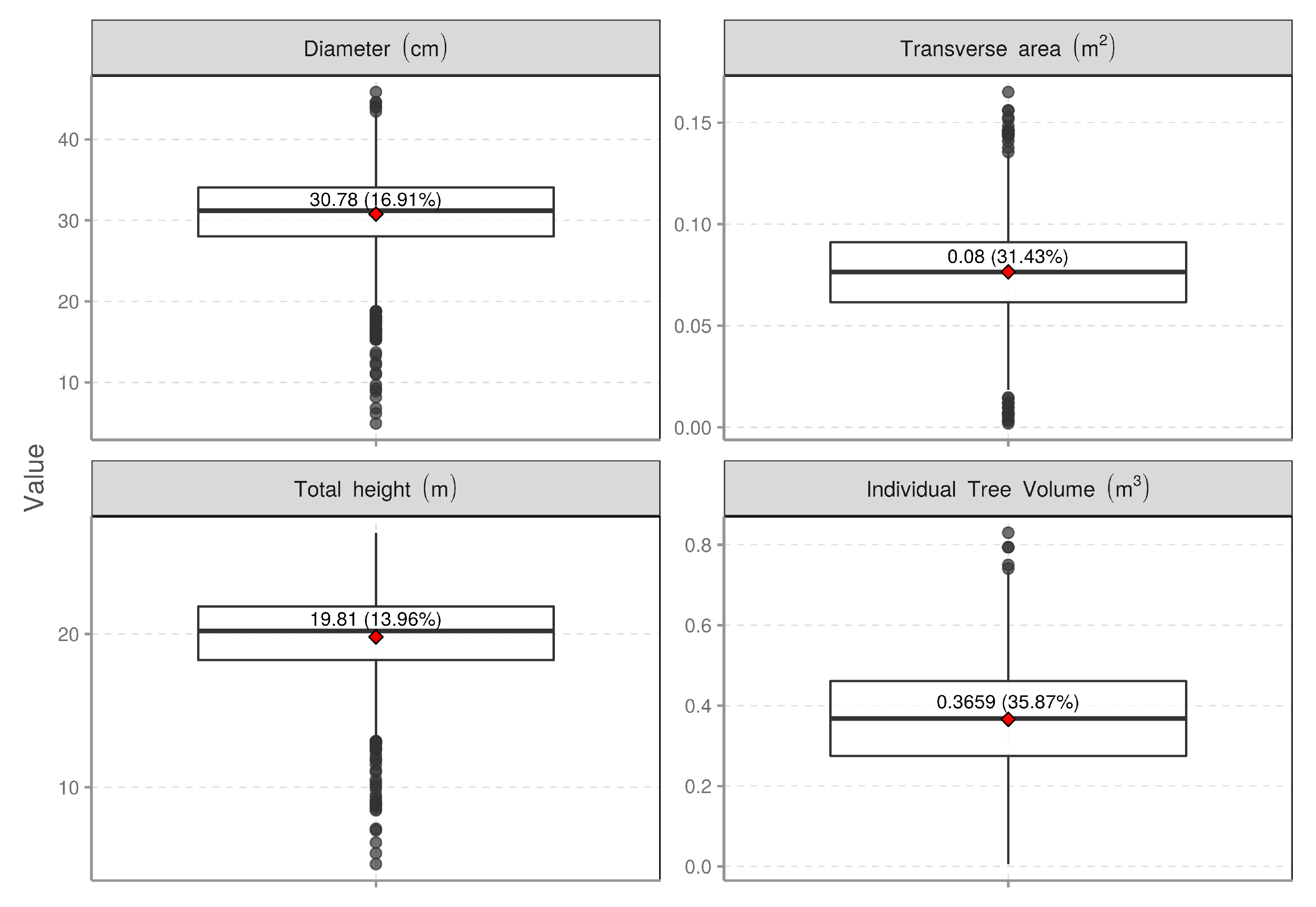
3.1. Exploratory Analysis at Stand-Level

Figure 4 contends the box-plot of dendrometric values for the stand. The average diameter of the trees in the plantation was 30.78 cm with a coefficient of variation (CV) of 16.91% and the average transverse area was 0.08 m² with a CV of 31.43%. The average total height was 19.81 m (CV = 13.96%) and the average individual volume was 0.3659 m³ (CV = 35.87%).

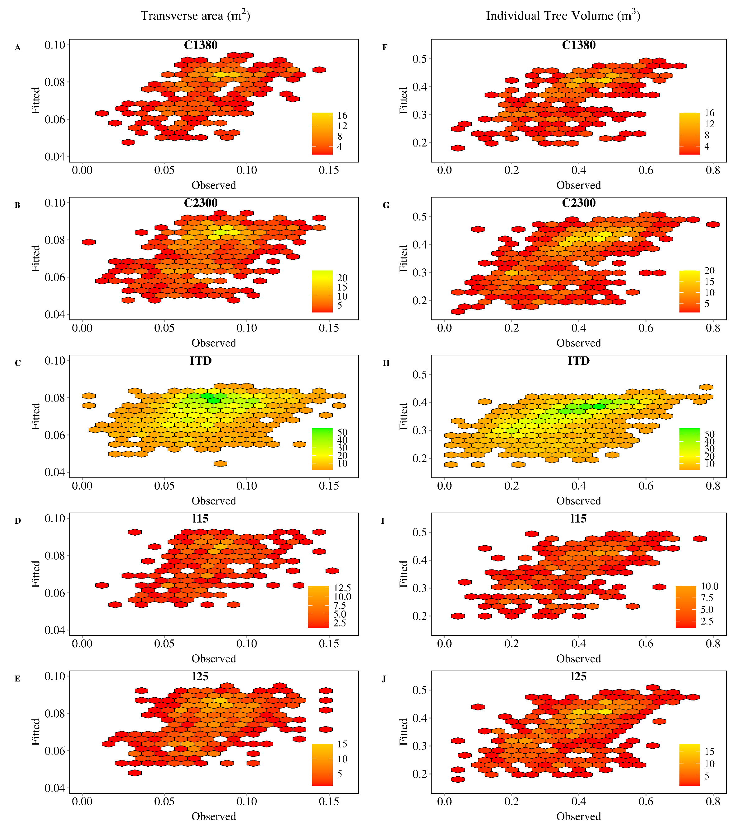
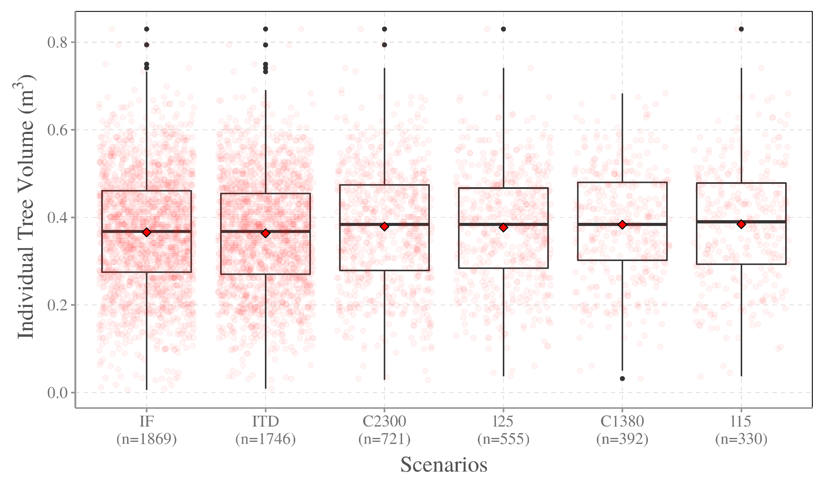
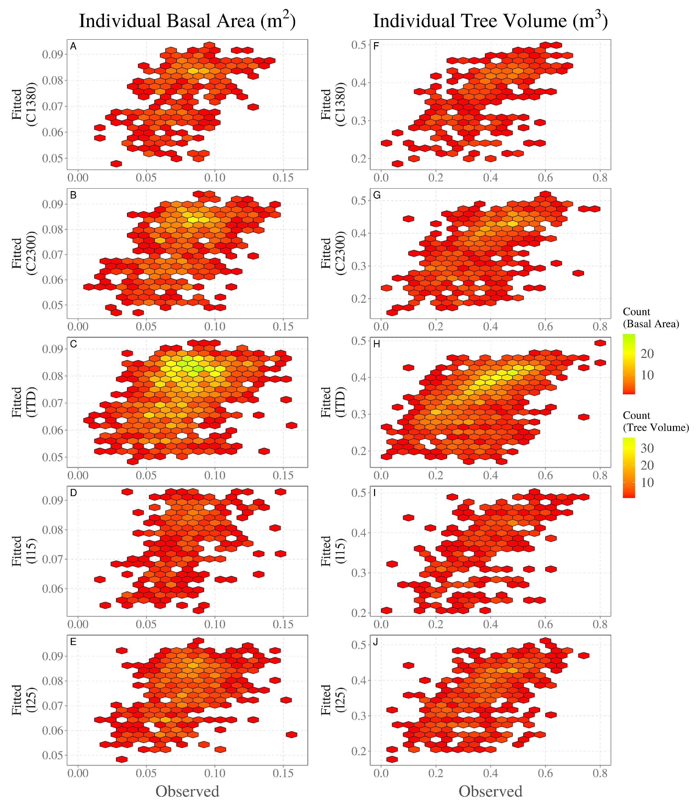
3.2. Individual Tree Volume Estimation in the Scenarios

The complete census (IF) totaled 1869 trees with an average individual volume of 0.3659 m³ (with minimum and maximum values of 0.0059 and 0.8300 m³, respectively) according to Figure 5. In general, all scenarios performed statistically similar for individual tree volume IF (vmi = 0.3659 m³), ITD (vmi = 0.3947 m³), C2300 (vmi = 0.3791 m³), L25 (vmi = 0.3769 m³), C1380 (vmi = 0.3833 m³) and L15 (vmi = 0.3843 m³). The data demonstrated homogeneity of variance and normality, and these averages of individual tree volumes showed no significant differences, so was accepted (p = 0.013). Although the sampling scenarios (Circular plots and Linear plots) had a lower number of trees sampled (ns = 721, 555, 392, 330) compared to the forest inventory based on a complete census (n = 1869), they were still able to represent the individual tree volumes. The ITD scenario, on the other hand, identifies 1746 individuals.

The performance of observed (IF) and tested scenarios for transverse areas indicated a Relative Root Mean Square Error (RMSE) between 0.0191 m² as a minimum value and 0.0217 m² as a maximum value (

Table 1. Summary of the estimation results of basal area and volume for the stand.

Variable	Scenario	R2	Syx	Syx%	RMSE	RMSE%	Bias	Bias%	r	x2	AIC	n
Transverse area	C1380	0.2433	0.0088	11.2158	0.0191	24.4770	0.0025	3.2397	0.4932	2.1181	2722.76	392
	C2300	0.2356	0.0126	16.1565	0.0202	25.9988	0.0030	3.8794	0.4854	6.1981	5103.52	721
	ITD	0.1418	0.0218	28.3185	0.0225	29.2833	0.0038	4.9757	0.3766	17.2681	−2758.33	1746
	l15	0.1935	0.0084	10.5888	0.0199	25.1861	0.0025	3.2069	0.4398	1.8080	2283.539	330
	l25	0.1850	0.0113	14.4168	0.0208	26.4420	0.0028	3.5814	0.4301	3.3561	3835.496	555
Volume	C1380	0.3614	0.0465	12.1434	0.1016	26.5015	0.0164	4.2665	0.6012	13.9608	−674.585	392
	C2300	0.4156	0.0641	16.8959	0.1031	27.1886	0.0169	4.4693	0.6447	26.5454	−1224.52	721
	ITD	0.3142	0.1060	29.1596	0.1096	30.1530	0.0217	5.9776	0.5605	84.9910	937.2128	1746
	l15	0.3479	0.0461	11.9887	0.1096	28.5159	0.0189	4.9288	0.5899	14.5701	−516,812	330
	l25	0.3390	0.0577	15.3074	0.1058	28.0754	0.0177	4.7079	0.5822	22.0331	−912.18	555

). Pearson’s correlation coefficient (r) varied between 0.3982 and 0.4932. Standard error of estimate in percentage (Syx%) varied between 10.5888 and 24.4946%. For the individual tree volume, the RMSE had values between 0.1016 m³ and 0.1096 m³. Pearson’s correlation coefficient (r) varied between 0.5730 and 0.6447. Standard error of estimate in percentage (Syx%) varied between 11.9887 and 25.5509%.

Figure 6 shows the dispersion of the transverse area (Figure 6a–e) between the observed values (IF) and the tested scenarios (ITD, C1380, C2300, L15, L25) and individual tree volume (Figure 6f–j) between the observed values (IF) and the tested scenarios (ITD, C1380, C2300, L15, L25). We notice a similar behavior among all scenarios in tending to underestimate the transverse area when using the LiDAR metrics, since the Y-axis scale has lower values.

Figure 7a–e shows the differences in basal area between each scenario evaluated (ITD, C1380, C2300, L15, L25) in comparison with field data (FI). Figure 7f–j shows the difference between individual tree volume and the scenarios tested (ITD, C1380, C2300, L15, L25).

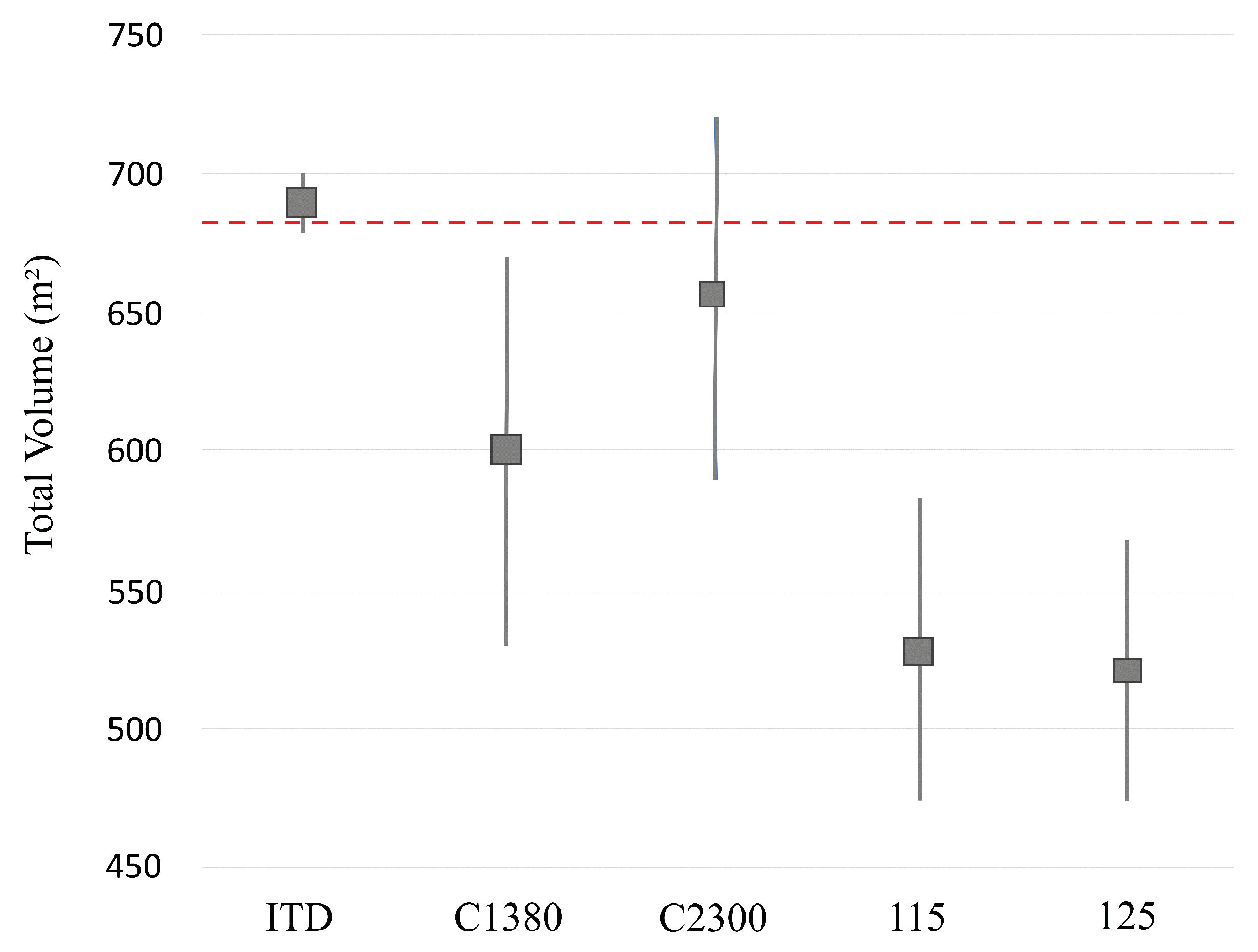
3.3. Estimates for the Forest Stand

The ITD scenario was the closest to the field values (1869) in terms of number of trees n = 1746 (with a difference of −6.58%), and in second order C2300 with n = 1728 (with a difference of −7.54%). Of these trees in the field, we have 20 forked trees and 9 trees without canopy, i.e. 1840 normal trees (forest inventory based on a complete census). Under these conditions, the differences would be reduced to −5.1 (ITD) and −6.09% (C2300).

On the forest stand scenario, (

Table 2. Summary of the estimation results of basal area and volume for the stand.

		Scenarios
Variable	Statistc	ITD	C1380	C2300	l15	l25
* Number 113 n ha−1	x(n ha−1)	106	95	104	83	84
1869	X(n)	1746	1566	1728	1371	1383
* Basal area	x (m2 ha−1)	8.13	7.40	8.14	6.54	6.57
IF 8.65 m2 ha−1	CI lower (m2 ha−1)	8.01	6.78	7.60	6.04	6.16
	CI upper (m2 ha−1)	8.25	8.01	8.68	7.04	6.98
* Volume	x (m3 ha−1)	41.67	36.29	39.62	31.84	31.51
IF 41.34 m3 ha−1	CI lower (m3 ha−1)	40.98	32.06	35.67	28.42	28.66
686.88 m3	CI upper (m3 ha−1)	42.36	40.52	43.56	35.27	34.36
	X (m3)	689.29	600.21	655.23	526.71	521.24
	CI lower (m3)	677.87	530.22	589.97	470.12	583.29
	CI upper (m3)	700.71	670.21	720.50	474.10	568.38

* Reference values IF (forest inventory based on a complete census): Number of trees per ha: 113; Number total of trees: 1869; Basal area 8.65 m² ha⁻¹; Volume by hectare: 41.34 m³ ha⁻¹; Volume by stand: 683.88 mm³.

), it was observed that the basal area values ranged from 7.40 m² ha⁻¹ (C1380) to 8.14 m² ha⁻¹ (C2300), about −5.9% less than the real value (8.65 m² ha⁻¹). It is also highlighted that all scenarios underestimated the basal area values. The C2300 scenario was the only one whose confidence interval limits included the basal area real value (8.65 m² ha⁻¹) in its amplitude (7.60 to 8.68 m² ha⁻¹).

Likewise for the total stand volume, the ITD scenario was the one that presented the closer values (689.29 m³) to the real total value (683.88 m³) with the real value positioned in the range of the confidence interval (677.87 to 700.71 m³). The C2300 scenario was ranked second with a volume of 655.23 m³ and intervals between 589.97 and 720.50 m³.

Considering the confidence intervals of the forest inventory for 95% probability (Figure 8) the C2300 and ITD scenarios were the ones with confidence intervals that contemplated the parametric mean volume, both per hectare and for total area. In the case of basal area only the c2300 approach had confidence intervals that covered the parametric value.

4. Discussion

The use of laser scanning sensors on UAV platforms has gained great prominence for forest inventory [22,28]. In this study we present an approach to measure three stand parameters (volume, number of trees, and basal area) by means of a UAV-LiDAR system for integrated crop-livestock-forest system. To date, this is the first study that presents an approach for UAV-LiDAR cloud sampling in ILPF systems. To do this, we created the SFI approach, which takes into account a simple cloud sampling system and applies the principles of the ITD approach; that is, instead of applying ITD to the entire area, we apply it only to a set of samples (plots), and subsequently expand it to the total area. We expect this approach to be a practical way for companies that are automating their FI data collection processes through UAV-LiDAR systems. The reduction of field effort, especially plot data collection, implies saving a large amount of money and faster processing with high accuracy [45]. The results obtained from this pilot study have demonstrated potential for application in forest inventories and forest management assistance.

Our results confirm that the estimates obtained using the SFI equates with the results obtained in ITD under certain conditions, and that both approaches (SFI and ITD) proved to be useful techniques showing satisfactory bias, RMSE, and Pearson’s coefficient between observed and estimated values for modeling individual volume and cross-sectional area. First, we estimated the mean volume (Figure 5) for each scenario, and found that all scenarios have mean values statistically similar to the FI. Then, we expanded to the stand the total number of individuals and noticed that only the ITD and the C2300 scenarios showed values close to the total number of individuals in the area. In this context, we realized that the critical point of the approach is related to the size of the plot that probably does not present sufficiency in the number of individuals. In addition to a probable insufficiency in the number of individuals in the plot, errors of commission and omission may have occurred because of the ITD approach, as well as adjustment parameters, and the stand structure itself. In recent years, several studies have highlighted the potential of using UAVs for vegetation mapping at small and large scales [22,28,46,47,48]. In particular using LiDAR data for ITD, accurate results have been found depending on forest conditions [49,50].

At the stand level, the results showed the same direction, the ITD approach and the C2300 scenario were the best suited to faithfully represent tree number, basal area and volume, and showed no significant differences between each other. Such a result reveals that the accuracy of UAV-LiDAR estimates increased with plot size for ILPF stands. At best, the transverse area was best served in the C1380 scenario (R² = 0.24; RMSE = 24.47%), followed by the C2300 scenario (R² = 0.23; RMSE = 25.99%), while for Volume, the best result was seen for C2300 (R² = 0.41; RMSE = 27.18%), followed by the C1380 scenario (R² = 0.36; RMSE = 26.50%). Despite a paucity of literature on ILPF stand inventory, our results for BA were consistent with previous work that showed the R² ranging from 0.29–0.57 across different species types [51].

Furthermore, evaluating and discussing the accuracy of our results in relation to established work was a complex task due to the literature for ILPF systems. However, in comparison with studies that have evaluated the influence of sample size, we note that our findings are quite comparable with the inferences made by other studies. In [45] was evaluated the impact of sample size and also modeling approaches and found that model performance was sensitive to sample size, and that an increase in R² occurred as sample size increased. In the case of our study, it can be seen that using an optimal number of sample trees from the evaluation, will provide greater accuracy, appearing to be a more efficient strategy for forest management [52,53]. It is important to comment that tree spacing in ILPF type systems is greater than in traditional stands, and that the SFI approach that takes into account larger plots may be more suitable for these conditions, given the tree spacing. While in small plots, the individuals present within this type of sampling unit appear to be insufficient to represent the stand. The total number of individuals in the area was also best represented by ITD and SFI C2300; the other approaches were not able to represent the count of individuals, most likely due to the same aspects presented.

The following aspects may have affected the results of this study. First, the insufficient number of trees contained in the plots in the SFI approach, i.e., it was possible to describe the parameters reliably only in the circular plot condition with an area of 2300 m². In addition, a potential positioning error of the subjects may also have caused some deviations in the results, the improvement of which depends on the equipment and data processing methods. GPS errors associated with tree location estimation are a common source of uncertainty that needs further investigation [54]. Also, the issue of ITD limitations with its dependence on stand structure, in our case irregular branching forms of the eucalypt species may have caused omission and commission when outlining trees, which are common errors in ITD algorithms [55,56].

Future work perspectives could address the lack of approaches for forest inventory under iCLFconditions with UAV-LiDAR, since most of the developed work is applied in homogeneous plantations at traditional spacings [45]. Furthermore, in our work we presented a perspective for forest inventory focusing on the parameters volume, number of individuals and basal area, however, upcoming work could explore for example biomass and carbon estimation and also the increments in carbon stocks of iCLF plantations in multitemporal contexts. Additional tests are therefore needed to increase confidence in the methodology and generalize it—for example, in other forest systems and also in evenly spaced stands. Alternative modeling and sampling techniques could also be explored; for instance, AI techniques could show better results since they deal better with the non-normalization of the data, as well as a bootstrapping sampling system could resample the data, generating a more robust model. Finally, we still recommend adding topographical variables in uneven terrain situations, since the DTM can be easily obtained in processing.

Finally, the overall accuracy of this study proved the feasibility of the proposed approach, and confirmed the use of a UAV as a promising alternative for inventory for an integrated crop-livestock-forest system. The SFI approach can be very useful in acquiring the stand parameters, as well as being a strategic means for processing high-density LiDAR clouds. Thus, future work with UAV-LiDAR data can benefit in acquiring forest volume at regional scales at relatively low cost.

5. Conclusions

This work compares two approaches—Sampling Forest Inventory and Forest Inventory based on a complete Census—to predict the individual mean volume and the basal area of an eucalyptus stand in a crop-livestock-forest system by using UAV-LiDAR data. Both methods allowed us to address an important barrier: tree counting and attribute estimation (volume and basal area) on wide-spaced stands.

The findings of our study indicate that for conditions prevalent in an integrated crop-livestock-forest system, the SFI approach (C2300) that considers an area of 2300 m² is suitable to generate estimates at the same level as the ITD approach.

It was found that plot sampling techniques need to have a large area to be appropriate in an integrated crop-livestock-forest system. This was the situation for the 2300 m² circular plots. Since the individual mean values were statistically equal for all approaches, the difference was caused by the number of trees captured by the plots.

Individual tree detection (ITD) approaches also proved to be suitable for generating the volume, with the values being very close to the actual values. This approach was the one that most closely matched the number of trees in the stand.

The authors recommend that future work should test the performance of applying high-density UAV-Lidar to forest inventories in traditional commercial plantations.

References

1. Payn, T.; Carnus, J.M.; Freer-Smith, P.; Kimberley, M.; Kollert, W.; Liu, S.; Orazio, C.; Rodriguez, L.; Silva, L.N.; Wingfield, M.J. Changes in planted forests and future global implications. For. Ecol. Manag. 2015, 352, 57–67. [Google Scholar] [CrossRef] [Green Version]
2. Sanquetta, C.R.; Dalla Corte, A.P.; Pelissari, A.L.; Tomé, M.; Maas, G.C.B.; Sanquetta, M.N.I. Dynamics of carbon and CO2 removals by Brazilian forest plantations during 1990–2016. Carbon Balance Manag. 2018, 13, 20. [Google Scholar] [CrossRef] [PubMed] [Green Version]
3. Indústria Brasileira de Àrvores (IbÀ). Annual Report. 2020. Available online: https://iba.org/datafiles/publicacoes/relatorios/relatorio-iba-2020.pdf (accessed on 15 September 2020).
4. Schmidt, L.N.; Sanquetta, M.N.I.; McTague, J.P.; da Silva, G.F.; Fraga Filho, C.V.; Sanquetta, C.R.; Scolforo, J.R.S. On the use of Weibull distribution in modeling and describing diameter distributions of clonal eucalypt stands. Can. J. For. Res. 2020, 50, 1050–1063. [Google Scholar] [CrossRef]
5. Silverio, F.O.; Barbosa, L.C.A.; Silvestre, A.J.D.; Pilo-Veloso, D.; Gomide, J.L. Comparative Study On The Chemical Composition Of Lipophilic Fractions From Three Wood Tissues Of Eucalyptus Species By Gas Chromatography-Mass Spectrometry Analysis. J. Wood Sci. 2007, 53, 533–540. [Google Scholar] [CrossRef]
6. Zago, L.M.S.; Ramalho, W.P.; Caramori, S. Does crop-livestock-forest systems contribute to soil quality in Brazilian Savannas? Floresta Ambiente 2019, 26, e20180343. [Google Scholar] [CrossRef]
7. Tonini, H.; Wink, C.; Silva, A.G.M.F. Sampling alternatives for eucalyptus trees in integrated crop-livestock-forest system. Floresta Ambiente 2019, 26, e20170893. [Google Scholar] [CrossRef] [Green Version]
8. Lafiti, H.; Heurich, M. Multi-scale remote sensing-assisted forest inventory: A glimpse of the state-of-the-art and future prospects. Remote. Sens. 2019, 11, 1260. [Google Scholar]
9. Kangas, A. Model-based inference. In Forest Inventory, Methods and Applications. Managing Forest Ecosystems; Springer: Dordrect, The Netherlands, 2006; Chapter 3; Volume 10, pp. 39–52. [Google Scholar]
10. White, J.; Coops, N.C.; Wulder, M.A.; Vastaranta, M.; Hilker, T.; Tompaski, P. Remote sensing technologies for enhancing forest inventories: A review. Can. J. Remote Sens. 2016, 42, 619–641. [Google Scholar] [CrossRef] [Green Version]
11. Næsset, E. Predicting forest stand characteristics with airborne scanning laser using a practical two-stage procedure and field data. Remote Sens. Environ. 2002, 80, 88–99. [Google Scholar] [CrossRef]
12. Asner, G.P.; Mascaro, J. Mapping tropical forest carbon: Calibrating plot estimates to a simple LiDAR metric. Remote Sens. Environ. 2014, 140, 614–624. [Google Scholar] [CrossRef]
13. Nilsson, M. Estimation of tree heights and stand volume using an airborne LiDAR system. Remote Sens. Environ. 1996, 56, 1–7. [Google Scholar] [CrossRef]
14. Zimble, D.A.; Evans, D.L.; Carlson, G.C.; Parker, R.C.; Grado, S.C.; Gerard, P.D. Characterizing vertical forest structure using small-footprint airborne LiDAR. Remote Sens. Environ. 2003, 87, 171–182. [Google Scholar] [CrossRef] [Green Version]
15. Latifi, H.; Heurich, M.; Hartig, F.; Müller, J.; Krzystek, P.; Jehl, H.; Dech, S. Estimating over-and understorey canopy density of temperate mixed stands by airborne LiDAR data. For. Int. J. For. Res. 2016, 89, 69–81. [Google Scholar] [CrossRef] [Green Version]
16. Hernández-Stefanoni, J.L.; Dupuy, J.M.; Johnson, K.D.; Birdsey, R.; Tun-Dzul, F.; Peduzzi, A.; López-Merlín, D. Improving species diversity and biomass estimates of tropical dry forests using airborne LiDAR. Remote Sens. 2014, 6, 4741–4763. [Google Scholar] [CrossRef] [Green Version]
17. Rex, F.E.; Corte, A.P.D.; Machado, S.D.A.; Silva, C.A.; Sanquetta, C.R. Estimating Above-Ground Biomass of Araucaria angustifolia (Bertol.) Kuntze Using LiDAR Data. Floresta Ambiente 2019, 26. [Google Scholar] [CrossRef]
18. Bayat, B.; van der Tol, C.; Yang, P.; Verhoef, W. Extending the SCOPE model to combine optical reflectance and soil moisture observations for remote sensing of ecosystem functioning under water stress conditions. Remote Sens. Environ. 2019, 221, 286–301. [Google Scholar] [CrossRef]
19. Lim, K.; Treitz, P.; Wulder, M.; St-Onge, B.; Flood, M. LiDAR remote sensing of forest structure. Prog. Phys. Geogr. 2003, 27, 88–106. [Google Scholar] [CrossRef] [Green Version]
20. Dandois, J.P.; Olano, M.; Ellis, E.C. Optimal altitude, overlap, and weather conditions for computer vision UAV estimates of forest structure. Remote Sens. 2015, 7, 13895–13920. [Google Scholar] [CrossRef] [Green Version]
21. Sankey, T.; Donager, J.; McVay, J.; Sankey, J.B. UAV LiDAR and hyperspectral fusion for forest monitoring in the southwestern USA. Remote Sens. Environ. 2017, 195, 30–43. [Google Scholar] [CrossRef]
22. Cunha Neto, E.M.; Rex, F.E.; Veras, H.F.P.; Moura, M.M.; Sanquetta, C.R.; Käfer, P.S.; Sanquetta, M.N.I.; Zambrano, A.M.A.; Broadbent, E.N.; Corte, A.P.D. Using high-density UAV-LiDAR for deriving tree height of Araucaria Angustifolia in an Urban Atlantic Rain Forest. Urban For. Urban Green. 2021, 63, 127197. [Google Scholar] [CrossRef]
23. Shinzato, E.T.; Shimabukuro, Y.E.; Coops, N.C.; Tompalski, P.; Gasparoto, E.A. Integrating area-based and individual tree detection approaches for estimating tree volume in plantation inventory using aerial image and airborne laser scanning data. iFor. Biogeosci. 2017, 10, 296–302. [Google Scholar] [CrossRef] [Green Version]
24. Picos, J.; Bastos, G.; Míguez, D.; Alonso, L.; Armesto, J. Individual tree detection in a eucalyptus plantation using unmanned aerial vehicle (UAV)-LiDAR. Remote Sens. 2020, 12, 885. [Google Scholar] [CrossRef] [Green Version]
25. Jeronimo, S.M.A.; Kane, V.R.; Churchill, D.J.; McGaughey, R.J.; Franklin, J.F. Aplicando a detecção de árvores individuais LiDAR ao manejo de paisagens florestais estruturalmente diversas. J. For. 2018, 116, 336–346. [Google Scholar]
26. Cosenza, D.N.; Soares, V.P.; Leite, H.G.; Gleriani, J.M.; Amaral, C.H.d.; GrippJúnior, J.; Silva, A.A.L.d.; Soares, P.; Tomé, M. Airborne laser scanning applied to eucalyptus stand inventory at individual tree level. Pesqui. Agropecu. 2018, 53, 1373–1382. [Google Scholar] [CrossRef]
27. Zheng, W.; Chen, J.; Hao, Z.; Shi, J. Comparative analysis of the chloroplast genomic information of Cunninghamia lanceolata (Lamb.) Hook with sibling species from the Genera Cryptomeria D. Don, Taiwania Hayata, and Calocedrus Kurz. Int. J. Mol. Sci. 2016, 17, 1084. [Google Scholar] [CrossRef] [PubMed] [Green Version]
28. Dalla Corte, A.P.; Souza, D.V.; Rex, F.E.; Sanquetta, C.R.; Mohan, M.; Silva, C.A.; Zambrano, A.A.; Prata, G.; de Almeida, D.R.A.; Trautenmüller, J.W.; et al. Forest inventory with high-density UAV-LiDAR: Machine learning approaches for predicting individual tree attributes. Comput. Electron. Agric. 2020, 179, 105815. [Google Scholar] [CrossRef]
29. Empresa Brasileira de Pesquisa Agropecuária (EMBRAPA). Sistema Brasileiro de Classificação de Solos, 3rd ed.; Empresa Brasileira de Pesquisa Agropecuária: Brasília, Brazil, 2013; 353p. [Google Scholar]
30. United States Department of Agriculture. Natural Resources Conservation Service. Keys to Soil Taxonomy, 11th ed.; United States Department of Agriculture: Washington, DC, USA, 2010; 346p. [Google Scholar]
31. Alvares, C.A.; Stape, J.L.; Sentelhas, P.C.; Gonçalves, J.L.M.; Sparovek, G. Köppen’s climate classification map for Brazil. Meteorol. Z. 2013, 22, 711–728. [Google Scholar] [CrossRef]
32. Porfírio-da-Silva, V.; Medrado, M.J.S.; Nicodemo, M.L.F.; Dereti, R.M. Arborização de Pastagens com Espécies Florestais Madeiras: Implantação e Manejo; Embrapa Florestas: Colombo, Brasil, 2010; 48p. [Google Scholar]
33. Dalla Corte, A.P.; Rex, F.E.; de Almeida, D.R.A.; Sanquetta, C.R.; Silva, C.A.; Moura, M.M.; Wilkinson, B.; Zambrano, A.M.A.; da Cunha Neto, E.M.; Veras, H.F.P.; et al. Measuring individual tree diameter and height using GatorEye high-density UAV-LiDAR in an integrated crop-livestock-forest system. Remote Sens. 2020, 12, 863. [Google Scholar] [CrossRef] [Green Version]
34. Broadbent, E.N.; Almeyda Zambrano, A.M.; Omans, G.; Adler, B.; Alonso, P.; Naylor, D.; Chenevert, G.; Murtha, T.; Prata, G.; de Almeida, D.R.A.; et al. The GatorEye Uninhabited Flying Laboratory: Sensor Fusion for 4D Ecological Analysis through Custom Hardware and Algorithm Integration. Available online: www.gatoreye.org (accessed on 5 May 2021).
35. Isenburg, M. “LAStools—Efficient LiDAR Processing Software” (Version 1.8, Licensed). Available online: http://rapidlasso.com/LAStools (accessed on 11 November 2019).
36. Roussel, J.-R.; Auty, D. Airborne LiDAR Data Manipulation and Visualization for Forestry Applications R Package Version 3.1.2. 2021. Available online: https://cran.r-project.org/package=lidR (accessed on 21 August 2021).
37. Popescu, S.C.; Wynne, R.H. Seeing the trees in the forest. Photogramm. Eng. Remote Sens. 2013, 70, 589–604. [Google Scholar] [CrossRef] [Green Version]
38. Kangas, A.; Maltamo, M. Forest Inventory, Methodology and Applications; Springer: Dordrect, The Netherlands, 2009; 362p. [Google Scholar]
39. Kershaw, J.A.; Weiskittel, A.R.; Lavigne, M.B.; McGarrigle, E. An imputation/copula-based stochastic individual tree growth model for mixed species Acadian forests: A case study using the Nova Scotia permanent sample plot network. For. Ecosyst. 2017, 4, 1–13. [Google Scholar] [CrossRef] [Green Version]
40. Kvålseth, T.O. Cautionary note about R2. Am. Stat. 1985, 39, 279–285. [Google Scholar]
41. Pretzsch, H. Forest dynamics, growth, and yield. In Forest Dynamics, Growth and Yield; Springer: Berlin/Heidelberg, Germany, 2009; pp. 1–39. [Google Scholar]
42. Kuhn, M.; Johnson, K. Applied Predictive Modeling; Springer: Chicago, IL, USA, 2013; 810p. [Google Scholar]
43. Tanaka, S.; Takahashi, T.; Nishizono, T.; Kitahara, F.; Saito, H.; Iehara, T.; Awaya, Y. Stand volume estimation using the k-NN technique combined with forest inventory data, satellite image data and additional feature variables. Remote Sens. 2015, 7, 378–394. [Google Scholar] [CrossRef] [Green Version]
44. Zhang, J.; Chen, W.; Sun, P.; Zhao, X.; Ma, Z. Prediction of protein solvent accessibility using PSO-SVR with multiple sequence-derived features and weighted sliding window scheme. BioData Min. 2015, 8, 3. [Google Scholar] [CrossRef] [PubMed] [Green Version]
45. Silva, V.S.D.; Silva, C.A.; Mohan, M.; Cardil, A.; Rex, F.E.; Loureiro, G.H.; Klauberg, C. Combined impact of sample size and modeling approaches for predicting stem volume in eucalyptus spp. forest plantations using field and LiDAR data. An. Acad. Bras. Ciênc. 2020, 12, 1438. [Google Scholar]
46. Martínez-de Dios, J.R.; Merino, L.; Caballero, F.; Ollero, A. Automatic forest-fire measuring using ground stations and unmanned aerial systems. Sensors 2011, 11, 6328–6353. [Google Scholar] [CrossRef] [PubMed] [Green Version]
47. Panagiotidis, D.; Abdollahnejad, A.; Surový, P.; Chiteculo, V. Determining tree height and crown diameter from high-resolution UAV imagery. Int. J. Remote Sens. 2017, 38, 2392–2424. [Google Scholar] [CrossRef]
48. Mohan, M.; Silva, C.A.; Klauberg, C.; Jat, P.; Catts, G.; Cardil, A.; Dia, M. Individual tree detection from unmanned aerial vehicle (UAV) derived canopy height model in an open canopy mixed conifer forest. Forests 2017, 8, 340. [Google Scholar] [CrossRef] [Green Version]
49. Silva, C.A.; Klauberg, C.; Hudak, A.T.; Vierling, L.A.; Liesenberg, V.; Carvalho, S.P.E.; Rodriguez, L.C. A principal component approach for predicting the stem volume in Eucalyptus plantations in Brazil using airborne LiDAR data. For. Int. J. For. Res. 2016, 89, 422–433. [Google Scholar] [CrossRef]
50. Liang, X.; Litkey, P.; Hyyppa, J.; Kaartinen, H.; Vastaranta, M.; Holopainen, M. Automatic stem mapping using single-scan terrestrial laser scanning. Meteorol. Z. 2012, 22, 711–728. [Google Scholar] [CrossRef]
51. Jevšenak, J.; Skudnik, M. A random forest model for basal area increment predictions from national forest inventory data. For. Ecol. Manag. 2021, 479, 118601. [Google Scholar] [CrossRef]
52. Hou, Z.; Mehtätalo, L.; McRoberts, R.E.; Ståhl, G.; Tokola, T.; Rana, P.; Siipilehto, J.; Xu, Q. Remote sensing-assisted data assimilation and simultaneous inference for forest inventory. Remote Sens. Environ. 2019, 234, 111431. [Google Scholar] [CrossRef]
53. Maltamo, M.; Mehtätalo, L.; Vauhkonen, J.; Packalén, P. Predicting and calibrating tree attributes by means of airborne laser scanning and field measurements. Can. J. For. 2012, 42, 1896–1907. [Google Scholar] [CrossRef]
54. Lisein, J.; Pierrot-Deseilligny, M.; Bonnet, S.; Lejeune, P. A photogrammetric workflow for the creation of a forest canopy height model from small unmanned aerial system imagery. Forests 2013, 4, 922–944. [Google Scholar] [CrossRef] [Green Version]
55. Goerndt, M.E.; Monleon, V.J.; Temesgen, H. Relating forest attributes with area- and tree-based light detection and ranging metrics for Western Oregon. West. J. Appl. For. 2010, 25, 105–111. [Google Scholar] [CrossRef] [Green Version]
56. Véga, C.; Durrieu, S. Multi-level filtering segmentation to measure individual tree parameters based on LiDAR data: Application to a mountainous forest with heterogeneous stands. Int. J. Appl. Earth Obs. Geoinf. 2011, 13, 646–656. [Google Scholar] [CrossRef] [Green Version]
Figure 1. Study area location and stand characterization in the State of Paraná, southern Brazil.
Drones 06 00048 g001
Figure 2. Methodological approaches tested and illustrative diagram of UAV-LiDAR point cloud and ITD processing. (a) UAV-LiDAR point cloud pre-processing; (b) Generation of Digital Terrain Model (DTM) and Digital Surface Model (DSM); (c) Generation of Canopy Height Model (CHM); (d) Individual tree detection (ITD); (e) LiDAR-derived tree height (hLiDAR) using ITD dat; (f) Extract hLiDAR; (g) Clip of samples plots.
Drones 06 00048 g002
Figure 3. Point cloud processing diagram for the different approaches and analyses performed.
Drones 06 00048 g003
Figure 4. Box-plot for the variables diameter (cm), transverse area (m2), total height (m), and volume (m3) for the stand.
Drones 06 00048 g004
Figure 5. Box-plot for the individual tree volumes in different scenarios. Where: Black points represent outlier values; Red points represent average values; Pink points represent the observations in the scenarios; IF = forest inventory based on a complete census; ITD = individual tree detection; C2300 = circular plots had areas of 2300 m2; L25 = linear plots had fixed tree numbers of 25 individuals; C1380 = circular plots had areas of 1380 m2; L15 = linear plots had fixed tree numbers of 15 individuals.
Drones 06 00048 g005
Figure 6. Dispersion count between observed (IF) and the tested scenarios for transverse area and individual tree volume. Where: Counts represents maps the number of cases to the hexagon fill.
Drones 06 00048 g006
Figure 7. Differences between each scenario evaluated compared to the field data (FI).
Drones 06 00048 g007
Figure 8. Means and confidence intervals for the variables basal area, volume per hectare, and total volume. The red line represents the parametric values (based on a complete census).
Drones 06 00048 g008