Autonomous Surveying of Plantation Forests Using Multi-Rotor UAVs

Abstract

Modern plantation forest procedures still rely heavily on manual data acquisition in the inventory process, limiting the quantity and quality of the collected data. This limitation in collection performance is often due to the difficulty of traversing the plantation forest environment on foot. This work presents an autonomous system for exploring plantation forest environments using multi-rotor UAVs. The proposed method consists of three parts: waypoint selection, trajectory generation, and trajectory following. Waypoint selection is accomplished by estimating the rows’ locations within the environment and selecting points between adjacent rows. Trajectory generation is completed using a non-linear optimization-based constant speed planner and the following is accomplished using a model predictive control approach. The proposed method is tested extensively in simulation against various procedurally generated forest environments, with results suggesting that it is robust against variations within the scene. Finally, flight testing is performed in a local plantation forest, demonstrating the successful application of our proposed method within a complex, uncontrolled environment.

1. Introduction

Modern plantation forestry is an industry with the explicit goal of maximizing the yield of high-quality wood within a managed area. One part of plantation forest management is the forest inventory process used to estimate the volume of merchandisable timber within a plot of trees. Successful application of this will provide the forester with data to identify any issues with the volumetric growth rate and to make an informed decision regarding the forest harvest date. In New Zealand, forest inventories are conducted using the regression-based analysis technique MARVL [1], where systematic sampling is used to select small groups of trees for extrapolating data regarding the entire forest. This sampling process is known as cruising and is generally completed on foot using manual means [2], which is subject to cost and labor availability limitations. In pursuit of higher accuracies and more frequent surveys, modern methods have moved towards better parameter estimation methods with plot imputation [3], which calibrates large-scale aerial surveys using ground data. Some existing forms of data collection used are Airborne Laser Scanning (ALS) [4,5], Terrestial or Mobile Laser Scanning (TLS/MLS) [6,7] to collect the aerial and ground calibration data.

Unfortunately, the under-canopy environment is a hostile environment for humans and ground-based robots due to uneven terrain, branching, and undergrowth, all of which are seen in the plantation forests shown in Figure 1. The presence of these obstacles means that ground-based traversal within plantation forests is heavily impeded, resulting in slow and expensive under-canopy data acquisition. Fortunately, recent advancements in UAV technologies have produced low-cost, high-agility multi-rotor UAVs suitable for operation within complex environments such as plantation forests. With new sensors and processing methods capable of accurately capturing surrounding spatial information in real-time, multi-rotor UAVs carrying these sensors are rapidly gaining popularity in recent literature as remote sensors.

Existing literature regarding the operation of UAVs within under-canopy environments can be approximately split into two categories; the first category generally focuses on the mapping or data extraction aspects, and the second consists of works related to enabling autonomous flight or navigation within the forest. In general, works related to data capture in this area use manual flight with either LiDAR [8,9,10], or Stereo Vision/Structure from Motion [11,12,13]. These works usually aim to produce a survey-grade map so that parameters such as tree count, diameter at breast height, and tree taper can be extracted. The second set of works consists of those attempting to fly in forests autonomously; production of survey-grade maps and extraction of parameters are secondary in these works, with the main focus on safely traversing through the forest. Literature regarding the autonomous navigation of multi-rotor UAVs within under-canopy environments is relatively scarce, likely due to the niche use case and lack of advanced see and avoid capabilities of commercial multi-rotor systems. Nevertheless, projects such as [14] used a Hokuyo UTM-30LX 2D Planar LiDAR and an Artificial Potential Field (APF) controller for obstacle avoidance with a target velocity vector. A similar approach is followed in [15] using the same 2D LiDAR setup with a vector field-based controller for navigation. Both of these systems achieved autonomous flight between two rows of trees without collision. Similarly, [16,17] both also use a rigidly mounted 2D LiDAR for environmental sensing, coupled with GraphSLAM [18] for motion estimation in the environment. However, all of the previously noted projects only attempt to localize and implement see-and-avoid systems as opposed to fully navigating the environment for a complete survey.

Outside of the forestry space, general-purpose trajectory planning and exploration is an active area of research in robotics. In particular, optimization-based methods are rapidly gaining popularity as they can rapidly produce safe, dynamically feasible trajectories. The general methodology followed is to formulate a cost function related to the trajectory, its derivatives, and some form of collision penalty. Various approaches are used throughout literature, for example, discrete waypoints [19], high-order polynomials with quadratic programming [20], b-splines with a local [21] or global [22] map, fixed-duration piecewise polynomials [23], and safe-corridors [24,25,26]. In particular, [20,22,24] demonstrate the ability to traverse unknown forest environments without collision autonomously but still require manual waypoint selection. General exploration of unknown environments is also an active area of research with many existing works; for example, [27,28] use a two-tiered approach, where frontiers are first extracted, and the order they are visited is decided by solving a traveling salesman problem. In [29], a library of motion primitives is used to search for positions with maximum information gain, while in [30,31,32] the search is instead conducted using rapidly-exploring random-trees (RRT) to sample the already explored region. More recently, probabilistic roadmaps (PRM) have also been explored in [33]. Unfortunately, generalized exploration methods often do not offer the best coverage performance, as shown in our previous paper [34].

This paper details the development of a UAV platform capable of autonomously exploring under-canopy environments within plantation forests to produce faster surveys. To achieve this goal, the navigation strategy outlined in our previous work [34] is extended to function in the absence of any structural assumptions about the forest. Specifically, the contributions of this work are as follows:

• A method for online waypoint placement for autonomous coverage planning in plantation forests
• A nonlinear optimization-based trajectory generation method to rapidly plan constant-speed, dynamically feasible, and safe trajectories within complex environments
• Experimental flight testing results in both simulation and a local plantation forest to verify the proposed method

Towards these contributions, Section 2 details the flown UAV hardware and methodologies used for autonomous navigation within the plantation. Section 3 details simulation environments and experiments used to determine the theoretical performance of the proposed system. Finally Section 4 details flight tests performed in an outdoor plantation environment to validate the proposed methods.

2. Materials and Methods

Because autonomous flight within plantation forests is a novel task, no sufficiently compact off-the-shelf hardware capable of carrying an appropriate LiDAR with sufficient onboard computer and endurance exists. As a result, a prototype multi-rotor UAV has been developed for flight testing of the proposed methodology, mainly out of necessity as it would allow a significantly larger margin of error before any collisions occurred. Unfortunately, the smaller UAV and comparatively heavy payload result in somewhat poor endurance, which can only be improved with lighter sensors or batteries with higher energy density. Figure 2 shows this survey UAV, consisting of a quadrotor with slightly tilted propellers for increased yaw authority. A Livox MID-70 LiDAR, along with an Intel Realsense T265 completes the sensor setup, and an Intel NUC handles onboard processing for autonomous flight. ROS Noetic [35] is used as the middleware for the software implementation, and R3Live [36] is used for pose estimation.

For clarity, the notation $\left\{F_X\right\}$, $\left\{F_Y\right\}$, $\left\{F_Z\right\}$ represents the right-hand X, Y, and Z axes in the ENU frame F. Position, orientation, and transformations to frame $\left\{Y\right\}$ from with respect to frame $\left\{X\right\}$ is denoted as ${}^Y{P}_X$, ${}^Y{R}_X$, and ${}^Y{T}_X$ respectively. The inertial frame $\left\{I\right\}$ is used as the fixed world frame, while $\left\{B\right\}$ defines the location of the flight controller. While additional fixed LiDAR and camera frames are used during the computation of pose estimates and mapping information, they are excluded for clarity.

For autonomous navigation, three tasks must be completed: waypoint selection, trajectory generation, and trajectory following. The first task generates the sequence of waypoints to be visited to explore the environment fully, the second task produces a collision-free and dynamically feasible flight plan to reach the goal, and the last task executes the generated trajectory. An overview of the proposed system is shown in Figure 3.

To ensure robust operations within any plantation environment, the proposed method does not use any priori information regarding the structure of the plantation environment. All mapping data used in a single flight is generated onboard and online during that flight using ranging data from the onboard LiDAR, and pose estimates are generated using R3Live. This work does not use Global Navigation Satellite Systems (GNSS) due to the lack of sufficient accuracy without a clear line of sight to the sky.

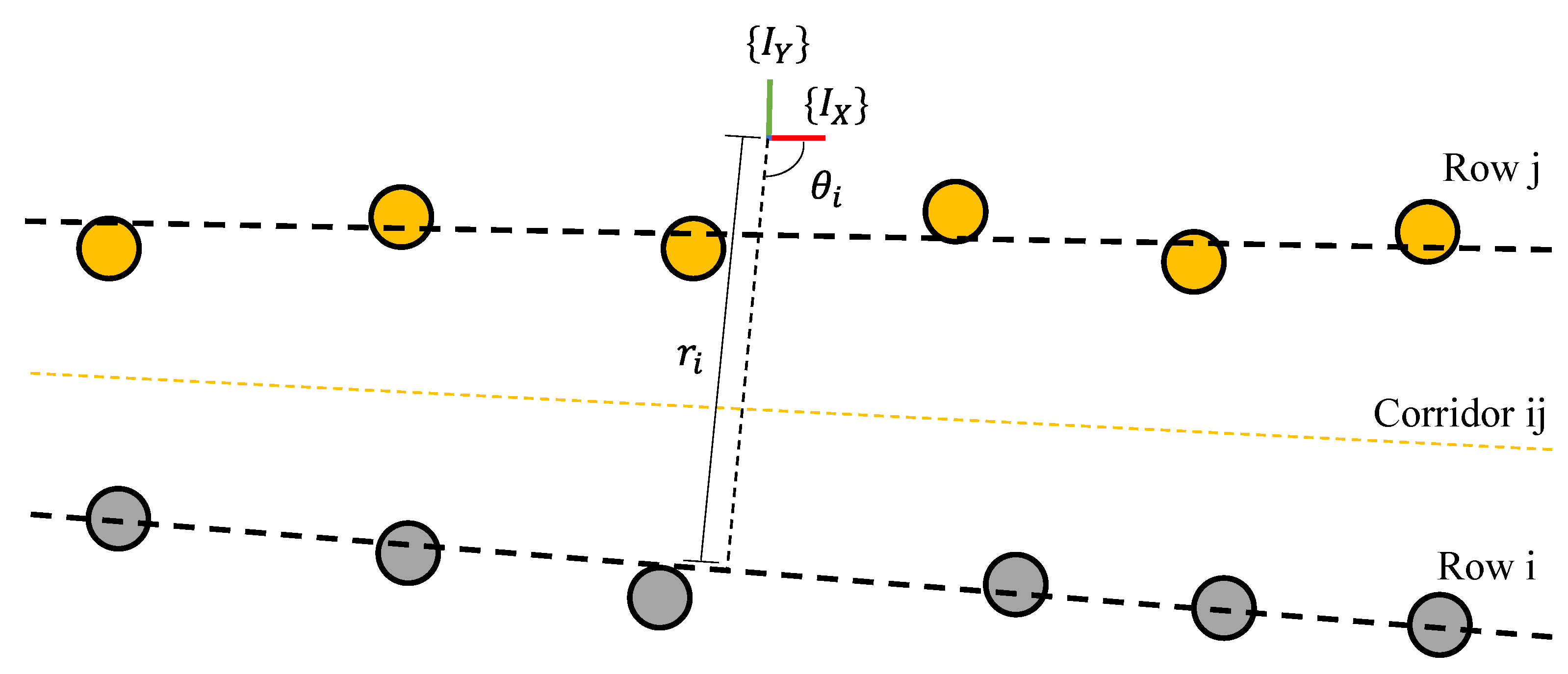
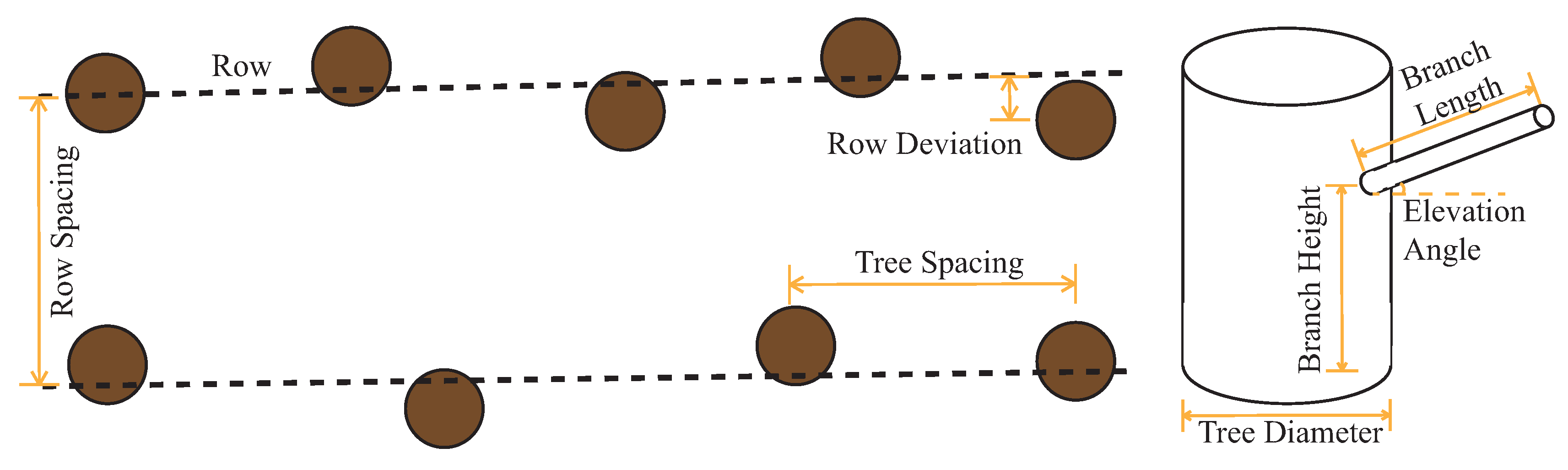
2.1. Waypoint Generation

Typical New Zealand plantation forests consist of Radiata pine ideally planted on a regularly spaced square grid to allocate an approximately equal land area to each tree. However, planting in a grid pattern is difficult, so real plantations are typically established on a row-by-row basis where trees are sequentially planted in parallel rows. This planting process produces distinct rows of trees with relatively consistent spacing between them but no consistent structure in the orthogonal direction, the effects of which can be seen in Figure 4.

Our previous work [34] introduces the concept of using a lawnmowing pattern aligned with the row direction to produce faster surveys, as shown in Figure 5. This work extends this concept to enable outdoor operation in realistic forests with irregular spaced rows. This task aims to produce a set of waypoints along the corridor between two adjacent rows of trees and to generate a new set of waypoints when the trajectory follower finishes executing the desired trajectory. The process of determining goal waypoints broadly consists of ground plane estimation and removal, tree clustering, row extraction, and finally, waypoint placement. It should be noted that while multi-UAV systems have the potential to greatly increase the coverage area through partitioning of the exploration space, they are outside of the scope of this work.

The first task of this process is ground plane estimation to remove the influence of ground elevation in the clustering process. The ground mesh is first estimated using Cloth Simulation Filter (CSF) [37] with the global occupancy grid serving as the input point cloud. Ground elevation can then be removed from the global point cloud by subtracting the corresponding estimated elevation, resulting in all estimated ground points occupying an elevation of 0m. Next, individual parallel rows of trees are identified through clustering to produce an estimate of the flight corridor between adjacent rows. A slice can then be taken from the elevation corrected point cloud and flattened to form a planar view of the forest at the current UAV altitude. DBSCAN [38] is then used to cluster these points to produce a list of estimated tree locations ${\mathit{C}}_{\mathit{s}}$. A search-based approach is used to determine the most likely direction of rows; consider the scenario presented in Figure 6, the stem locations can be collapsed along $\left\{I_X\right\}$ to form distinct clusters, as shown.

Given the good alignment of the row direction with $\left\{I_X\right\}$, distinct clusters will be observed in the collapsed state as shown in Figure 6a. Alternatively, if the row alignment is poor, the case in Figure 6b will be present, with fewer large clusters present in the scene. Thus, the most probable row direction consists of the direction that minimizes the spread of each present cluster. Using the sum of the spread of each cluster as a cost function, a search can be performed to determine the best alignment between $\left\{I_X\right\}$ and the estimated row directions. The functions for this are shown in Equations (1) and (2), optimizing for minimum cost.

$$\begin{array}{c}argminJ\left(\theta \right)=\frac{n_c}{n_v}\sum _{j=0}^{n_c}{((\max \left({\mathit{L}}_{\mathit{j}}\right)-\min \left({\mathit{L}}_{\mathit{j}}\right))/n_j)}^2\\ \mathrm{where}\end{array}$$

(1)

$$\mathit{L}=DBSCAN({\mathit{C}}_{\mathit{s}}\times \left[\begin{array}{c}sin\left(\theta \right)\\ cos\left(\theta \right)\end{array}\right]);{\mathit{C}}_{\mathit{s}}=\left[\begin{array}{cc}{x}_1& y_1\\ x_2& y_2\\ ⋮\\ x_{n_c}& y_{n_c}\end{array}\right][x_i,y_i]={}^{C_i}{P}_I$$

(2)

where ${\mathit{L}}_{\mathit{j}}$ denotes the list of transformed tree locations corresponding to cluster j, $n_j$ denotes the number of trees in cluster j, $n_v$ denotes the number of clusters with more than five trees, and $n_c$ denotes the number of clusters. Since row estimates are generated based on identified cluster information, the accuracy of the $\theta$ estimate does not need to be high. Because this work does not consider initial traversal to the survey starting location, an assumption is made that the inertial frame $\left\{I_x\right\}$ is approximately aligned with the row direction. Therefore, a coarse search is performed for $\theta \in [-{30}^{\circ },{30}^{\circ }]$ in 1° increments. The cluster labels from the minimum cost $\theta$ value are used to label the unmodified tree locations C, resulting in clusters of tree locations corresponding to independent rows. Finally, a least-squares fit is used to determine the estimated rows present within the scene and converted into the $r,\theta$ representation, as shown in Equations (3) and (4).

Let $\mathit{x}=\left[\begin{array}{c}m\\ c\end{array}\right]$ be the least squared solution to Ax = B

$$\mathit{A}=\left[\begin{array}{cc}{x}_1& 1\\ x_2& 1\\ ⋮\\ x_n& 1\end{array}\right];\mathit{B}=\left[\begin{array}{c}{y}_1\\ y_2\\ ⋮\\ y_n\end{array}\right]\mathrm{For}\mathit{L}=\{{\mathit{L}}_{\mathbf{1}},{\mathit{L}}_{\mathbf{2}},\cdots ,{\mathit{L}}_{\mathit{n}}\},x_i,y_i\in {\mathit{L}}_{\mathit{j}}$$

$$\theta =atan2(1,-m)$$

(3)

$$r=c\times sin\left(\theta \right)$$

(4)

As all segmented rows are approximately parallel, their relative position in the environment can be determined by sorting the list of rows by their associated r. Consider the environment shown in Figure 7, consisting of two approximately parallel rows ordered by r. Defining

$$\begin{array}{c}{r}_{ij}=0.5(r_i+r_j)\end{array}$$

(5)

$$\begin{array}{c}{\theta }_{ij}=0.5({\theta }_i+{\theta }_j)\end{array}$$

(6)

where $r_{ij},{\theta }_{ij}$ defines the estimated parameters of the traversal corridor between the tree rows defined by $r_i,r_j$. Since each corridor needs to be traversed at least once to fully explore the environment, the traversal order for N corridors then becomes $\{r_{12},r_{23},\cdots ,r_{N-1,N}\}$. Lastly, a set of waypoints can be established for traversal down a single corridor using Equations (7)–(9).

$$\begin{array}{c}\mathrm{Let}{\mathit{w}}_{\mathit{s}}={\{0,Y\left(0\right),Z(0,Y\left(0\right))+Z_r\}}^T,{\mathit{w}}_{\mathit{e}}={\{0,Y\left(m\right),Z(m,Y\left(m\right))+Z_r\}}^T\end{array}$$

$$\begin{array}{c}Y\left(x\right)=x\times tan({90}^{\circ }-{\theta }_{ij})+\frac{r_{ij}}{sin\left({\theta }_{ij}\right)}\end{array}$$

(7)

$$\begin{array}{c}{\mathit{w}}_{\mathit{i}}=\left|{\mathit{w}}_{\mathit{d}}\right|\times m_{inc}+{\mathit{w}}_{\mathit{s}}\mathrm{For}i>0,i\le \frac{m}{m_{inc}}\end{array}$$

(8)

$$\begin{array}{c}{\mathit{w}}_{\mathit{d}}=\left\{\begin{array}{cc}{\mathit{w}}_{\mathit{e}}-{\mathit{w}}_{\mathit{s}}\hfill & mod(i,2)=1\hfill \\ {\mathit{w}}_{\mathit{s}}-{\mathit{w}}_{\mathit{e}}\hfill & \mathrm{otherwise}\hfill \end{array}\right.\end{array}$$

(9)

where $Z(x,y)$ is the estimated ground elevation at $\{I_x,I_y\}=\{x,y\}$, $Z_r$ is the reference altitude above ground, $m_{inc}$ is the spacing between successive waypoints, $w_i$ denotes the ith waypoint down a single corridor, and $w_s,w_e$ denotes the start and end coordinates for a single corridor. Each successive corridor is traversed in the reverse direction to remove the need to return before each traversed row. The generated list of waypoints is passed to the trajectory planner, where any occupied waypoints are skipped; the traversal of a single corridor is considered complete when the entire generated trajectory has been fully executed, or no additional waypoints can be visited. Exploration is terminated when the required number of rows is surveyed, and a waypoint at $\{0,0,Z(0,0\left)\right\}$ is sent to command a return to the origin.

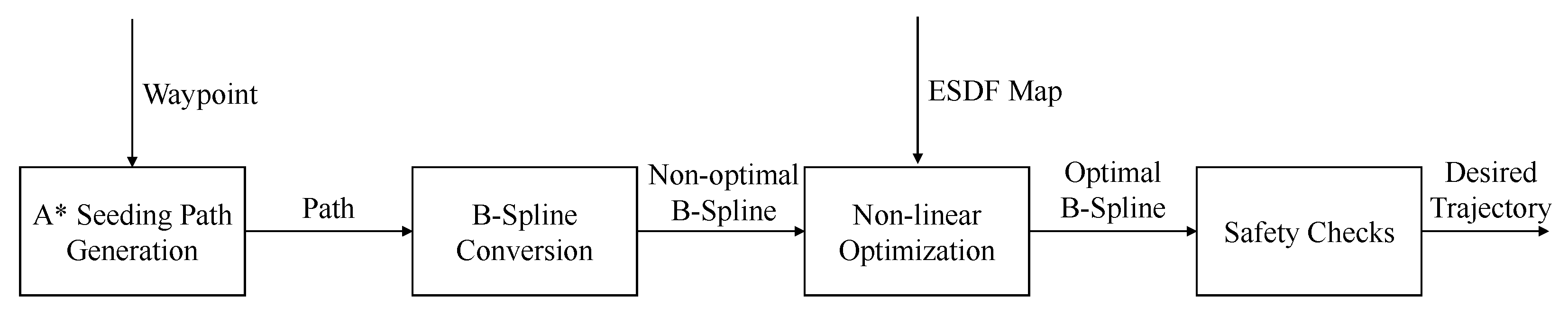
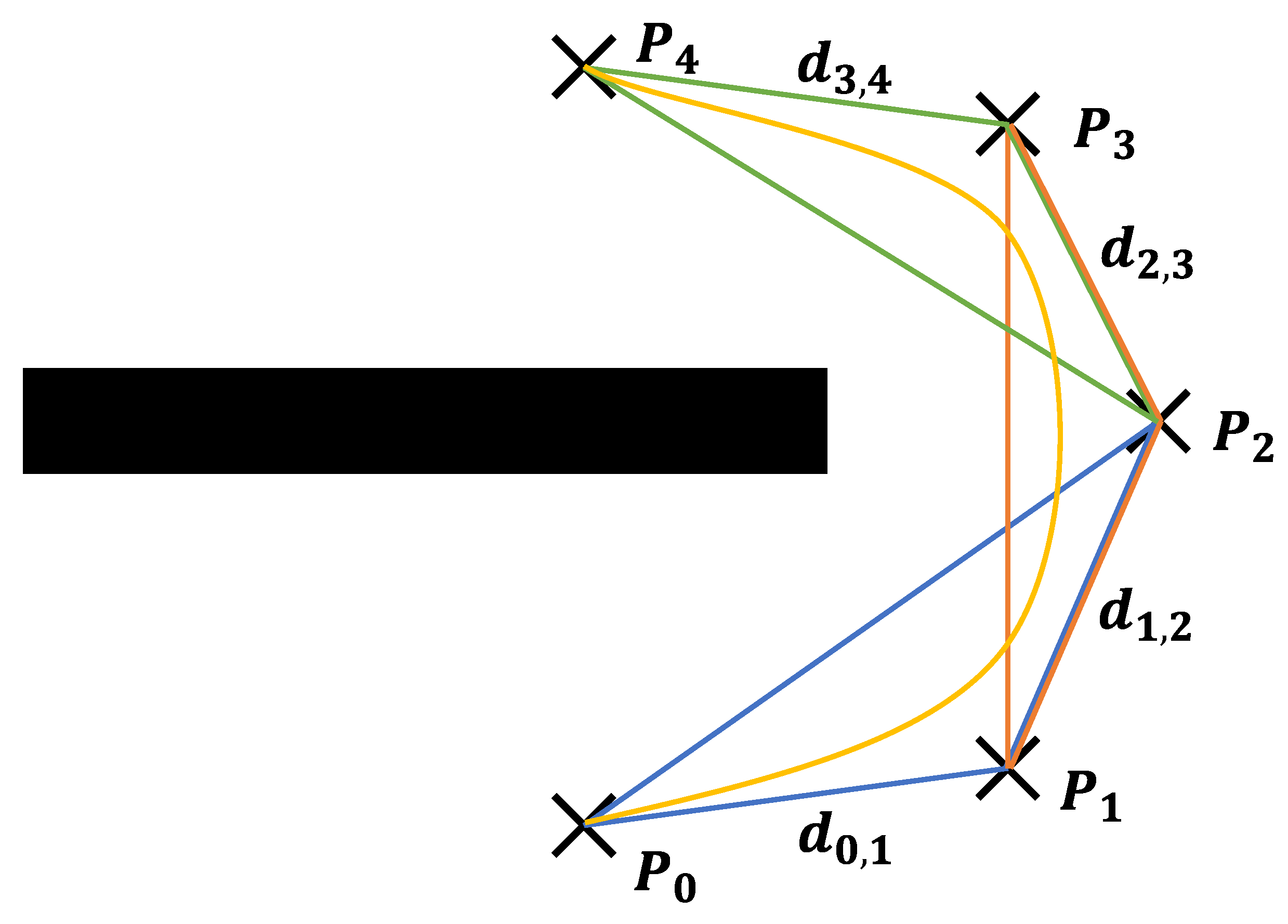
2.2. Trajectory Generation

The trajectory planner performs three tasks; maintaining an up-to-date global map of the environment, generating the actual flight trajectory, and finally replanning if the trajectory becomes unsafe. The pipeline overview is presented in Figure 8 and uses an optimization-based approach to generate high-quality trajectories rapidly. In line with many other optimization-based trajectory planners, a Euclidean Signed Distance Field (ESDF) is used for mapping information. The ESDF is built online with point cloud data from the MID-70 LiDAR using FIESTA [39].

Trajectories are represented as uniform clamped B-Splines, which are often used to define smooth curves using a small number of discrete points. A B-Spline is defined by the evenly spaced knot vector $\mathit{t}$ with interval $t_{int}$ and control points ${\mathit{P}}_{\mathbf{0}},{\mathit{P}}_{\mathbf{1}},\cdots {\mathit{P}}_{\mathit{n}}$ where ${\mathit{P}}_{\mathit{i}}$ represents a position in 3D space such that ${\mathit{P}}_{\mathit{i}}\in {\mathbb{R}}^3$, where:

$$\begin{array}{c}\mathit{t}=\{t_0,t_1,\cdots t_m\},t_{i+1}-t_i=t_{int};i\in [0,m-1]\end{array}$$

(10)

$$\begin{array}{c}\mathit{P}=\{{\mathit{P}}_{\mathbf{0}},{\mathit{P}}_{\mathbf{1}},\cdots {\mathit{P}}_{\mathit{n}}\}\end{array}$$

(11)

Departing from how B-Splines are typically defined, the knot vector is not constrained to $[0,1)$ and is instead defined such that $t_i\in [0,t_m)$. This definition of the knot vector is convenient because it allows for direct time allocation of the trajectory during optimization. B-Splines offer some beneficial properties in the context of trajectory planning, particularly C^N-1 continuity, and the strong convex hull property. A degree 3 B-Spline guarantees C² continuity at all points, which means that the trajectory is guaranteed to be continuous up to the 2nd derivative. The convex hull property also guarantees that any points of the spline will fall within the convex hull formed by the neighboring control points. Specifically, if $t\in [t_i,t_i+1)$, all points in that piecewise portion of the B-Spline are contained entirely in the convex hull formed by control points $P_{i-2},P_{i-1},P_i$. These properties greatly simplify the enforcement of collision constraints and dynamic limits.

The first step in the trajectory generation process is producing a seeding path, with the only requirement being that this path is collision-free and approximately optimal, since the shape and dynamic properties of the trajectory will be heavily modified during optimization. It should be noted, however, that this solution should ideally be close to the optimal path to increase the probability of the optimized trajectory converging on the global minima instead of less optimal local minima. Because these requirements are very loose, an A* search [40] in 3D using 26-way connectivity is performed with the Manhattan distance heuristic to rapidly generate a traversal path to the goal. For speed reasons, the A* search grid has the same voxel resolution as the ESDF (0.2m), allowing direct ESDF lookups to be used for occupancy checking. The output of this search is a discrete set of poses $\mathit{O}$ which encodes $n_o$ discrete positions in the inertial frame $\left\{I\right\}$ containing a collision-free path to the goal, namely

$$\mathit{O}={\{{\mathit{o}}_1,{\mathit{o}}_2,\cdots ,{\mathit{o}}_{n_o}\}}^T\mathrm{where}{\mathit{o}}_i=\left\{{}^{o_i}{P}_I\right\}$$

(12)

The generated path is used to seed the initial trajectory by creating a B-Spline with control points $\mathit{P}=\mathit{O}$, spaced equally at time interval $t_{int}$, initially set to 0.1 s.

It should be noted that A* is used in this work only for ease of implementation, therefore many other polynomial-time path-finding algorithms such as D* Lite, $\theta$*, JPS, Kinodynamic A*, etc. can be used in place of A* to generate the initial seeding path. However, probabilistic methods such as RRT(*) are less suitable as any initial solutions tend to be poor quality, and compute times are less predictable depending on the source and quality of available randomness, both of which affect the generation time and quality of the resulting trajectory.

Once the seeding B-Spline is created, the next step is to refine the trajectory to satisfy safety and dynamic constraints, as the only guarantee at this part of the process is collision safety. To refine the quality of this seeding trajectory, a non-linear optimization problem can be formulated around the B-Spline’s control points and time interval. Leveraging Google Ceres’ [41] Levenberg-Marquardt solver as a least-squares solver, the cost function $F\left(\mathit{x}\right)$ is defined as:

$$F\left(\mathit{x}\right)=F_{collision}\left(\mathit{x}\right)+F_{velocity}\left(\mathit{x}\right)+F_{acceleration}\left(\mathit{x}\right)+F_{time}\left(\mathit{x}\right)+F_{continuity}\left(\mathit{x}\right)$$

(13)

where the parameter vector $\mathit{x}$ is defined as:

$$\mathit{x}=\{{\mathit{P}}_0,{\mathit{P}}_1,{\mathit{P}}_2,\cdots ,t_{int}\}$$

(14)

Because the B-Splines are uniform with a fixed interval of $t_{int}$ between each successive control point, the trajectory can be re-timed during the optimization process by including the time interval as an optimization parameter. This decouples the time of the trajectory with the number of waypoints, allowing for more flexibility in the number of control points used. The inclusion of $F_{continuity}\left(\mathit{x}\right)$ is used to enforce end-to-end continuity when multiple waypoints are provided to the planner; this is set to 0 when only a single waypoint is supplied. When a single trajectory consists of multiple sequentially visited waypoints, the optimization problem becomes one with multiple end-to-end joined B-Splines, which appends additional control points and time intervals to the parameter vector, namely

$$\mathit{x}=\{{\mathit{P}}_{0,0},{\mathit{P}}_{0,1},\cdots ,{\mathit{P}}_{1,0},{\mathit{P}}_{1,1},\cdots ,t_{in{t}_0},t_{in{t}_1},\cdots \}$$

(15)

where ${\mathit{P}}_{i,j}$ denotes the ith control point, and $t_{in{t}_j}$ denotes the time interval of the jth B-Spline.

Collision constraints in the planner are formulated by exploiting the strong convex hull property to guarantee a safe trajectory without needing to conduct expensive collision checks across the entire trajectory. Consider the scenario presented in Figure 9, where a degree 3 B-Spline trajectory tightly wraps around a corner. The initial portion of the B-Spline must be contained within the triangle formed by ${\mathit{P}}_0$ to ${\mathit{P}}_2$. Suppose the distance between any two control points ${\mathit{P}}_i$ and ${\mathit{P}}_j$ is denoted $d_{i,j}$, the convex hull of the initial portion is guaranteed to collision-free if the ESDF distance at ${\mathit{P}}_i$ is greater than ${\sum }_{j=i}^{i+1}{d}_{j,j+1}$. Unfortunately, calculating $d_{i,j}$ becomes expensive quickly as it needs to be recomputed at every step, so a relaxed variant of this constraint is used; $d_{i,j}$ is assumed to be the same as the voxel grid resolution. Given voxel resolution $d_{vox}$, the seeding control points $\mathit{O}$ are separated by $d_{vox}$ due to the A* search resolution; as the seeding path is non-optimal, the actual distance between control points post-optimization will likely be less than $d_{vox}$. Therefore, it is likely that the trajectory will be collision-free as long as the ESDF distance $d_{ESDF}^{{\mathit{P}}_i}$ at every ${\mathit{P}}_i$ is greater than at least two times $d_{vox}$. Therefore, collision threshold $d_{col}$ can be used as a tuning factor trading off speed for safety; smaller values allow the UAV to take faster routes at the expense of a higher probability of unsafe trajectories. To prevent the execution of unsafe trajectories, a collision check is performed at discrete intervals, and the trajectory is rejected if any point fails this check. The collision cost is, therefore, defined as:

$$\begin{array}{c}{\mathit{F}}_{collision}\left(\mathit{x}\right)=\sum _{i=0}^n\left(G\left({\mathit{P}}_i\right)\right)\end{array}$$

(16)

$$\begin{array}{c}G\left({\mathit{P}}_i\right)=\left\{\begin{array}{cc}{W}_{collision}{(\left(d_{col}\right)-d_{ESDF}^{{\mathit{P}}_i})}^2\hfill & \mathrm{if}{d}_{ESDF}^{{\mathit{P}}_i}<d_{col}\hfill \\ 0\hfill & \mathrm{otherwise}\hfill \end{array}\right.\\ d_{col}\ge 2\times d_{vox}\end{array}$$

(17)

where $W_{collision}$ is the collision weight.

Velocity constraints are handled as a combination of initial/final state constraints, maximum velocity constraints, and speed constraints, namely:

$$F_{velocity}\left(\mathit{x}\right)=F_{initialVel}\left(\mathit{x}\right)+F_{finalVel}\left(\mathit{x}\right)+F_{speed}\left(\mathit{x}\right)+F_{maxVel}\left(\mathit{x}\right)$$

(18)

Because the B-Spline is C² continuous, the velocity at any point can be determined by inspecting the derivative of the B-Spline. The control point defining the velocity profile at index i can be computed based on the position control points ${\mathit{P}}_i$ and ${\mathit{P}}_{i+1}$ using the derivative of the position B-Spline. Because the convex hull property similarly constrains the velocity B-Spline, the profile’s maximum velocity is also constrained by the magnitude of the velocity control points. The velocity control points are defined by:

$$\begin{array}{c}{\mathit{P}}_i^{vel}=\frac{3}{int}({\mathit{P}}_{i+1}-{\mathit{P}}_i)\\ \mathrm{where}\\ int=\left\{\begin{array}{cc}{t}_{in{t}_i}\times (i+1)\hfill & \mathrm{if}i<3\hfill \\ t_{in{t}_i}\times (n-i-1)\hfill & \mathrm{if}i>(n-4)\hfill \\ t_{in{t}_i}\times 3\hfill & \mathrm{otherwise}\hfill \end{array}\right.\end{array}$$

(19)

Therefore, the velocity state at control point ${\mathit{P}}_i$, and the initial and final velocity can be constrained by Equation (20). The velocity weight $W_{velState}$ is set to a relatively large value to encourage constant speed traversal in the environment.

$$\begin{array}{c}{F}_{velState}(P_i^{vel},V_{ref})={\mathit{W}}_{velState}\left|\right|{\mathit{P}}_i^{vel}-{\mathit{V}}_{ref}{\left|\right|}^2\end{array}$$

(20)

$$\begin{array}{c}{F}_{initialVel}\left(\mathit{x}\right)=F_{velState}({\mathit{P}}_0^{vel},{\mathit{V}}_{initial})\end{array}$$

(21)

$$\begin{array}{c}{F}_{finalVel}\left(\mathit{x}\right)=F_{velState}({\mathit{P}}_{n-1}^{vel},{\mathit{V}}_{final})\end{array}$$

(22)

Because forest surveying is the intended use case of this trajectory planner, there is an additional speed constraint to encourage a constant trajectory speed for more even coverage of the environment. The speed constraint is implemented by $F_{speed}$, which penalizes the planner when the speed at any particular control point differs from the desired survey speed.

$$F_{speed}\left(\mathit{x}\right)=\sum _{i=0}^{n-1}{W}_{speed}\left(\right||{\mathit{P}}_{\mathit{i}}^{\mathit{vel}}\left|\right|-S_{ref})$$

(23)

where $S_{ref}$ is the scalar reference speed for the survey. Finally, the maximum velocity can be constrained by defining:

$$\begin{array}{c}{\mathit{F}}_{velMax}\left(\mathit{x}\right)=\sum _{i=0}^{n-1}sw{\mathit{W}}_{velMax}\left(\right|{\mathit{P}}_i^{vel}{|-{\mathit{V}}_{max})}^2\\ sw=\left\{\begin{array}{cc}1\hfill & \mathrm{if}\left|\right|{\mathit{P}}_i^{vel}\left|\right|>{\mathit{V}}_{max}\hfill \\ 0\hfill & \mathrm{otherwise}\hfill \end{array}\right.\end{array}$$

(24)

where ${\mathit{W}}_{velMax}$ is the velocity feasibility penalty weight; deliberately set large to discourage trajectories that violate dynamic limits.

Similarly, the acceleration B-Spline is simply the derivative of the velocity B-Spline, and the convex hull property still applies. Therefore, the acceleration control points and, by extension, maximum accelerations are defined as:

$$\begin{array}{c}{\mathit{P}}_i^{acc}=\frac{2}{in{t}_h}\left({\mathit{P}}_{i+1}^{vel}\right)-\frac{2}{in{t}_l}\left({\mathit{P}}_i^{vel}\right)\\ in{t}_l=\left\{\begin{array}{cc}{t}_{in{t}_i}\times i\hfill & \mathrm{if}i<3\hfill \\ t_{in{t}_i}\times (n-i)\hfill & \mathrm{if}i>(n-3)\hfill \\ t_{in{t}_i}\times 2\hfill & \mathrm{otherwise}\hfill \end{array}\right.\\ in{t}_h=\left\{\begin{array}{cc}{t}_{in{t}_i}\times (i+1)\hfill & \mathrm{if}(i-1)<3\hfill \\ t_{in{t}_i}\times (n-i-1)\hfill & \mathrm{if}i>(n-4)\hfill \\ t_{in{t}_i}\times 2\hfill & \mathrm{otherwise}\hfill \end{array}\right.\end{array}$$

(25)

The maximum acceleration is constrained to dynamic limits by:

$$\begin{array}{c}{\mathit{F}}_{accMax}\left(\mathit{x}\right)=\sum _{i=0}^{n-2}sw{\mathit{W}}_{accMax}\left(\right|{\mathit{P}}_i^{acc}{|-{\mathit{A}}_{max})}^2\\ sw=\left\{\begin{array}{cc}1\hfill & \mathrm{if}\left|\right|{\mathit{P}}_i^{acc}\left|\right|>{\mathit{A}}_{max}\hfill \\ 0\hfill & \mathrm{otherwise}\hfill \end{array}\right.\end{array}$$

(26)

where ${\mathit{W}}_{accMax}$ is the acceleration feasibility penalty weight; deliberately set large to discourage the optimizer from exceeding dynamic limits.

Lastly, continuity constraints must also be added to ensure smoothness when multiple B-Splines define the trajectory. For this, it is important to guarantee the B-Splines are continuous up to the second derivative at the joints. Thus, the overall continuity cost function can be defined as:

$${\mathit{F}}_{continuity}\left(\mathit{x}\right)={\mathit{F}}_{velCont}\left(\mathit{x}\right)+{\mathit{F}}_{accCont}\left(\mathit{x}\right)$$

(27)

Note that it is unnecessary to add a position constraint in the continuity cost function; let ${\mathit{P}}_i^j$ denote control point i of B-Spline j. Because the B-Spline is clamped, it is sufficient to set ${\mathit{P}}_0^{i+1}={\mathit{P}}_{n_i}^i$ for $i\in [0,n_s-1]$ to guarantee end-to-end position constraints. The optimization can then proceed by using ${\mathit{P}}_{n_i}^i$ in place of ${\mathit{P}}_0^{i+1}$. Velocity and acceleration constraints are handled similarly to initial and final velocity constraints, namely:

$$\begin{array}{c}{\mathit{F}}_{velCont}\left(\mathit{x}\right)=\sum _{i=0}^{n_s-1}{\mathit{W}}_{velCont}\left|\right|{\mathit{P}}_{n_i-1}^{ve{l}_i}-{\mathit{P}}_0^{ve{l}_i+1}\left|\right|\end{array}$$

(28)

$$\begin{array}{c}{\mathit{F}}_{accCont}\left(\mathit{x}\right)=\sum _{i=0}^{n_s-1}{\mathit{W}}_{accCont}\left|\right|{\mathit{P}}_{n_i-1}^{ac{c}_i}-{\mathit{P}}_0^{ac{c}_i+1}\left|\right|\end{array}$$

(29)

Because the planning process uses an incrementally built ESDF for collision safety, trajectories may become unsafe when new obstacles are observed and added to the map. Collision checks are therefore continuously performed at 20Hz on the currently executing trajectory to ensure the safety of the UAV. Since the ESDF encodes the distance to the nearest obstacles, the trajectory is collision-free as long as $d_{ESDF}^{\mathit{C}\left(t\right)}>d_{uav}+d_{tolerance}$ for $t\in [0,t_m]$ is guaranteed, where $d_{ESDF}^{\mathit{C}\left(t\right)}$ is the ESDF distance at point $\mathit{C}\left(t\right)$, $d_{uav}$ is the radius of the UAV, and $d_{tolerance}$ is the collision tolerance. In general, the thresholds are set such that $d_{col}>d_{uav}+d_{tolerance}$ to reduce the probability of a generated trajectory failing the collision check.

If a new collision is found, the trajectory can be split into two portions; the committed and uncommitted portion, as shown in Figure 10. The committed portion consists of two seconds of the trajectory immediately following the current time, and the remainder of the trajectory is the uncommitted portion. Modifying the committed portion of the trajectory generally requires aggressive control inputs from the trajectory follower and, therefore, should be avoided unless there is an immediate collision threat. The uncommitted portion, however, can be modified at any time without impacting control.

If the collision lies within the committed portion, the current trajectory is immediately aborted by splicing a soft-stop trajectory one second into the future. This soft-stop splice consists of a fixed number of control points with the start and end clamped to the splice location. Following this, a new trajectory is then generated from the current location to reach the goal waypoint. A less disruptive trajectory splice can be performed if the collision lies in the uncommitted portion. In this mode, a new trajectory is generated at the transition point between the committed and uncommitted portions such that the initial state of the newly optimized trajectory matches the currently executing trajectory at the splice point. This freshly generated trajectory can then be seamlessly spliced into the uncommitted portion of the current trajectory and does not produce a performance penalty, as the splice occurs outside of the control horizon.

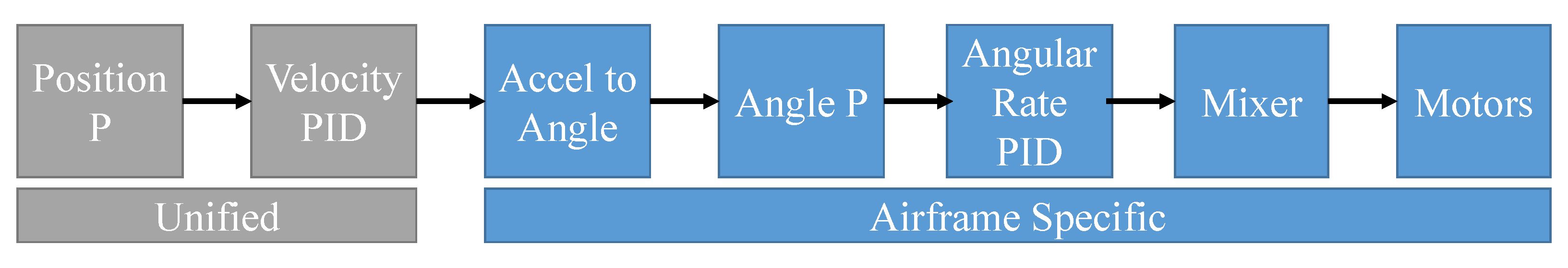
2.3. Trajectory Following

Once a trajectory has been generated, the UAV needs to be able to execute the generated trajectory accurately. Because of the groundwork laid in Section 2.2, it can be assumed that a collision-free, dynamically feasible trajectory is available ahead of time. A Model Predictive Control (MPC) trajectory controller using velocity setpoints for multi-rotor UAVs is used. The trajectory follower used is outlined in our previous paper [42]; therefore, this section will only briefly summarize the method. ACADO toolkit’s [43] code generation tool is used to generate an efficient solver that is run every timestep for the MPC implementation. In contrast to classical control methods for trajectory tracking, which are reactive in nature and can only attempt to minimize the current error, MPC is predictive, and attempts to minimize both the current and future error. This allows the controller to more accurately track complex trajectories that are known ahead of time.

The aim of this controller is to drive the body frame $\left\{B\right\}$ along a trajectory in SE3 space described by one or more B-Splines $\mathit{C}\left(t\right)$ in the inertial frame $\left\{I\right\}$ such that $\mathit{C}\left(t\right)={}^B{P}_I^{sp}$ at time t. Consider a simplified version of the cascaded controller shown below in Figure 11. The controller can effectively be split into two portions, the unified portion acting in inertial frame $\left\{I\right\}$, and the airframe-specific portions acting in body frame $\left\{B\right\}$. In many existing works, setpoints are injected at the angular rate level as each additional control loop produces additional latency. This work injects the setpoint at the velocity loop, producing distinct advantages. First, the setpoint is injected into the unified portion of the controller, so any airframes capable of tracking arbitrary velocity setpoints can be controlled without any modifications. Furthermore, attitude states no longer need to be tracked, as all control now occurs in the inertial frame.

Assuming the velocity loop is tuned appropriately, the entire airframe-specific portion can be collapsed into a first-order approximation, namely:

$$\begin{array}{c}\frac{\dot{{}^B{\mathit{P}}_I}}{\dot{{}^B{\mathit{P}}_I^{sp}}}=\frac{1}{\mathit{\tau }s+1}\\ \mathit{\tau }={\{{\tau }_X,{\tau }_Y,{\tau }_Z\}}^T\end{array}$$

(30)

where $\dot{{}^B{\mathit{P}}_I}$ is the velocity of body frame $\left\{B\right\}$ in inertial frame $\left\{I\right\}$, $\dot{{}^B{\mathit{P}}_I^{sp}}$ is the velocity setpoint, and $\mathit{\tau }\in {\mathbb{R}}^3$ is a vector of the velocity time constants in the body frame $\left\{B\right\}$. The overall architecture of the controller is presented in Figure 12, with position and velocity control provided by PX4’s internal controllers and feedback via PX4’s ECL.

The state vector $\mathit{x}$, and the system outputs $\mathit{y}$ is defined as:

$$\mathit{x}=\mathit{y}={\{{}^B{\mathit{P}}_I,\dot{{}^B{\mathit{P}}_I},\dot{{}^B{\mathit{P}}_I^{sp}}\}}^T$$

(31)

where $\dot{{}^B{\mathit{P}}_I}\in {\mathbb{R}}^3$ is the derivative of the position vector ${}^B{\mathit{P}}_I$, and ${\dot{{}^B{\mathit{P}}_I}}^{sp}$ is the reference velocity from the trajectory planner. The control input to the system is defined as:

$$\mathit{u}=\left\{\ddot{{}^B{\mathit{P}}_I^{sp}}\right\}$$

(32)

where ${\ddot{{}^B{\mathit{P}}_I}}^{sp}$ is the derivative of the velocity setpoint. Furthermore the reference trajectory can be packaged to define the reference system state ${\mathit{x}}^{ref}$ and ${\mathit{u}}^{ref}$:

$$\begin{array}{c}{\mathit{x}}^{ref}\left(t\right)={\{{}^B{\mathit{P}}_I^{ref},\dot{{}^B{\mathit{P}}_I^{ref}},\dot{{}^B{\mathit{P}}_I^{ref}}\}}^T=\{\mathit{C}\left(t\right),\dot{\mathit{C}\left(t\right)},\dot{\mathit{C}\left(t\right)}\}\end{array}$$

(33)

$$\begin{array}{c}{\mathit{u}}^{ref}\left(t\right)=\left\{{\ddot{{}^B{\mathit{P}}_I}}^{ref}\right\}=\left\{\ddot{\mathit{C}\left(t\right)}\right\}\end{array}$$

(34)

where $\ddot{{}^B{\mathit{P}}_I^{ref}}$, $\dot{{}^B{\mathit{P}}_I^{ref}}$, and ${}^B{\mathit{P}}_I^{ref}$ are the reference acceleration, velocity, and position of the reference trajectory $\mathit{C}\left(t\right)$ at time t.

The UAV model is formulated using the transfer function outlined in Equation (30), namely.

Let ${\mathit{A}}_{\mathit{m}},{\mathit{B}}_{\mathit{m}},{\mathit{C}}_{\mathit{m}},{\mathit{D}}_{\mathit{m}}$ describe the linear state-space system

$$\begin{array}{c}\dot{\mathit{x}}={\mathit{A}}_{\mathit{m}}\mathit{x}+{\mathit{B}}_{\mathit{m}}\mathit{u}\end{array}$$

(35)

$$\begin{array}{c}\mathit{y}={\mathit{C}}_{\mathit{m}}\mathit{x}+{\mathit{D}}_{\mathit{m}}\mathit{u}\\ {\mathit{A}}_{\mathit{m}}=\left[\begin{array}{ccc}0& \mathit{I}& 0\\ 0& -{\mathit{\tau }}_{\mathit{inv}}\mathit{I}& {\mathit{\tau }}_{\mathit{inv}}\mathit{I}\\ 0& 0& 0\end{array}\right]{\mathit{B}}_{\mathit{m}}=\left[\begin{array}{c}0\\ 0\\ \mathit{I}\end{array}\right]{\mathit{C}}_{\mathit{m}}=\left[\begin{array}{ccc}\mathit{I}& 0& 0\\ 0& \mathit{I}& 0\\ 0& 0& \mathit{I}\end{array}\right]{\mathit{D}}_{\mathit{m}}=0\end{array}$$

(36)

where $\mathit{I}\in {\mathbb{R}}^{3\times 3}$ is the 3 by 3 identity matrix, ${\mathit{\tau }}_{\mathit{inv}}\in {\mathbb{R}}^3$ is the element-wise inverse of vector $\mathit{\tau }$, and each 0 represents a 3-by-3 matrix of zeros. Let the sample time of the MPC controller be $t_s$ and the length of the optimization horizon be $t_s\times N$ where N is the number of samples; the optimization problem is formulated as:

$$\begin{array}{c}\mathrm{let}{\mathit{x}}_{\mathit{k}}^{\mathit{ref}}={\mathit{x}}^{ref}(k\times t_s),{\mathit{u}}_{\mathit{k}}^{\mathit{ref}}={\mathit{u}}^{ref}(k\times t_s)\\ argminJ\left(\mathit{x}\right)=\sum _{k=0}^{N-1}\left({\left({\mathit{x}}_{\mathit{k}}-{\mathit{x}}_{\mathit{k}}^{\mathit{ref}}\right)}^T\mathit{Q}\left({\mathit{x}}_{\mathit{k}}-{\mathit{x}}_{\mathit{k}}^{\mathit{ref}}\right)\right.+\left.{\left({\mathit{u}}_{\mathit{k}}-{\mathit{u}}_{\mathit{k}}^{\mathit{ref}}\right)}^T\mathit{R}\left({\mathit{u}}_{\mathit{k}}-{\mathit{u}}_{\mathit{k}}^{\mathit{ref}}\right)\right)\\ +{\left({\mathit{x}}_{\mathit{N}}-{\mathit{x}}_{\mathit{N}}^{\mathit{ref}}\right)}^T\mathit{P}\left({\mathit{x}}_{\mathit{N}}-{\mathit{x}}_{\mathit{N}}^{\mathit{ref}}\right)\\ \mathrm{subject}\mathrm{to}\\ {\mathit{x}}_{k+1}={\mathit{A}}_d{\mathit{x}}_{\mathit{k}}+B_d{\mathit{u}}_{\mathit{k}}\\ -{\mathit{v}}_{max}\le \dot{{}^B{\mathit{P}}_I^{ref}}\le {\mathit{v}}_{max}\\ -{\mathit{a}}_{max}\le \ddot{{}^B{\mathit{P}}_I^{ref}}\le {\mathit{a}}_{max}\end{array}$$

(37)

where ${\mathit{A}}_d$ and ${\mathit{B}}_d$ are the discrete-time variants of the state and input matrices ${\mathit{A}}_{\mathit{m}}$ and ${\mathit{B}}_{\mathit{m}}$, ${\mathit{x}}_k$ and ${\mathit{u}}_k$ is the predicted system state vector and control input vector at sample k. $\mathit{Q}\in {\mathbb{R}}^{9x9}$ and $\mathit{R}\in {\mathbb{R}}^{3x3}$ are the system state and control input weighting matrices, respectively, and are generally diagonal. $\mathit{P}\in {\mathbb{R}}^{9x9}$ is the solution to the algebraic Riccati equation. Vectors ${\mathit{v}}_{\mathit{max}}\in {\mathbb{R}}^3$ and ${\mathit{a}}_{\mathit{max}}\in {\mathbb{R}}^3$ are used to enforce hard limits on the velocity setpoint $\dot{{}^B{\mathit{P}}_I^{ref}}$ and rate of change of velocity setpoint $\ddot{{}^B{\mathit{P}}_I^{ref}}$.

To strike a balance between trajectory tracking performance and required onboard compute, the MPC formulation in this work uses sample time $t_s=0.1$ s and control and prediction horizon of 2 s, producing a total of $N=20$ steps in each optimization. To compensate for the relatively short optimization horizon, the controller is run at 50Hz using positions linearly interpolated along the reference trajectory.

The formulation outlined so far does not control the UAV’s yaw angle, as the UAV’s position and yaw angle are assumed to be decoupled. In reality, the yaw angle of the UAV must be continuously controlled to point in the direction of travel to guarantee safety. A simple P controller is used to control the yaw angle of the UAV and determined via Equation (38).

$$\dot{{\psi }^{sp}}=K_{\psi }({\psi }^{sp}-\psi )$$

(38)

where $\psi$ is the current yaw angle of the UAV, ${\psi }^{sp}$ is the yaw setpoint, $K_{\psi }$ is the yaw P gain, and $\dot{{\psi }^{sp}}$ is the yaw rate setpoint.

The yaw setpoint ${\psi }^{sp}$ is set such that the sensor is pointed towards the Euclidean center of the trajectory section between 1 to 2 s in the future, as shown in Equation (39).

$$\begin{array}{c}\mathrm{let}\mathit{V}\left(\mathit{t}\right)=\sum _{i=t+1}^{t+2}\left(\mathit{C}\left(t\right)\right)\\ {\psi }^{sp}=atan2(\mathit{V}\left(t\right)\left[1\right],\mathit{V}\left(t\right)\left[0\right])\end{array}$$

(39)

where $\mathit{V}\left(t\right)\left[1\right]$ is the y-axis value, and $\mathit{V}\left(t\right)\left[0\right]$ is the x-axis value of $\mathit{V}\left(t\right)$.

Because it is impossible to guarantee that the sensor is pointed in the correct direction without using an infinitely large yaw gain, a stall event is inserted when the setpoint leaves the horizontal FOV of the sensor. When this happens, the trajectory follower momentarily commands a zero velocity setpoint at the current position, and the yaw controller is given time to reorient the sensor. Trajectory tracking is resumed as soon as the sensor is oriented in the correct direction.

2.4. Runtime

It should be noted that the operating speed of the proposed method is generally limited by the availability of onboard computers, as safety of the UAV is dependent on the method continuously performing collision checks and generating new trajectories. In general, the most time-consuming task is the maintenance of the ESDF map, as a large number of voxels have to be sequentially updated. During simulation, the average optimization time for a single trajectory is approx. 30 ms, and varies with the length of the trajectory, while trajectory tracking takes approx. 250 us per step. In the event that faster cycle times are required, the resolution of the ESDF map or maximum sensor range, and the number of control points in the B-Spline could be reduced at the expense of requiring larger collision tolerances.

3. Simulation Tests

Simulation testing is conducted using Gazebo with PX4’s Software-In-The-Loop (SITL) environment via a simulated MID-70 sensor attached to the 3DR Iris model. The environments used for simulation are procedurally generated using the parameters acquired in [34], outlined in

Table 1. Summary of parameters extracted from plantation forest point clouds.

Parameter	Distribution Type	Mean(m)/a	SD(m)/b
Row spacing (m)	Gaussian	4.42	0.37
Row deviation (m)	Gaussian	0.01	0.78
Tree spacing (m)	Gamma	2.61	2.24
Branch length (Low-branching) (m)	Gamma	2.94	0.37
Branch length (High-branching) (m)	Gamma	7.31	0.37
Branch height (m)	Gaussian	4.76	1.01
Branch Elevation Angle (rad)	Gaussian	0.23	0.62
Tree diameter (m)	Gaussian	0.52	0.14

. A simplified view of these parameters in a forest environment are shown in Figure 13. A simulated ground plane is produced using Perlin Noise [44] to create cases with various terrain conditions. Three metrics are used to quantify the degree of each potential obstacle present in the environment, namely the amount of branching, the slope of the ground, and the roughness of the ground. Each of these metrics represents a relative comparison in difficulty, with higher values indicating a more challenging environment for traversal.

3.1. Branching

Aside from the stems, the most significant considered source of obstacles are low-hanging branches in the environment; branches that directly intrude on the available space between two rows of stems produce significantly more impact than those parallel to the rows. In particular, diagonal branches have a more significant effect than vertical or horizontal branches by creating larger zones where the UAV cannot traverse. Therefore, the branching metric is defined as the normalized sum of rectangular areas occupied in the perpendicular direction of the row as outlined in Equation (40).

Let ${\theta }_j,{\varphi }_j,l_j$ be the elevation and azimuth angle, and length of branch j

$$D_B\left(T\right)=\frac{1}{numTree}\sum _{i=0}^{numTree}\left(\sum _{j=0}^{numBranch}(sin\left({\varphi }_j\right){\left(l_j\right)}^{2}sin\left({\theta }_j\right)cos\left(\theta \right))\right)$$

(40)

where $numTree$ is the number of trees in the environment, and $numBranch$ is the number of branches corresponding to tree i.

3.2. Slope and Roughness

Since elevation changes heavily influence row segmentation and waypoint selection, any slope in the environment will increase the traversal difficulty. To define metrics describing the slope and roughness of each simulation testing environment. Consider a general plane representation

$$Z(x,y)=ax+by+c$$

(41)

where $a,b,c$ are dimensionless constants representing a least-squares fit of a plane in 3D space. Consider the ground plane as a list of i tuples $G=(x_0,y_0,z_0),(x_1,y_1,z_1),\cdots (x_i,y_i,z_i)$. The slope difficulty metric is described in Equation (42).

Let Ax = b be an over-constrained system

$$\begin{array}{c}\mathit{A}\in {\mathbb{R}}^{i\times 3},x\in {\mathbb{R}}^3,b\in {\mathbb{R}}^i\\ \mathrm{where}\\ \mathit{A}=\left[\begin{array}{ccc}{x}_0& y_0& 1\\ x_1& y_1& 1\\ & ⋮& \\ x_i& y_i& 1\end{array}\right]\mathit{x}=\left[\begin{array}{c}a\\ b\\ c\end{array}\right]\mathit{b}=\left[\begin{array}{c}{z}_0\\ z_1\\ ⋮\\ z_i\end{array}\right]\end{array}$$

$$D_s\left(G\right)=atan\left(\sqrt{a^2+b^2}\right)$$

(42)

Roughness is defined as the RMS of the difference between the plane’s estimated elevation at position $(x,y)$ compared to the actual ground elevation. The roughness of the ground plane is therefore defined as

$$D_r\left(G\right)=\sqrt{\sum _{k=0}^i\left({(F_z(x_k,y_k)-\left(z_k\right))}^2\right)}$$

(43)

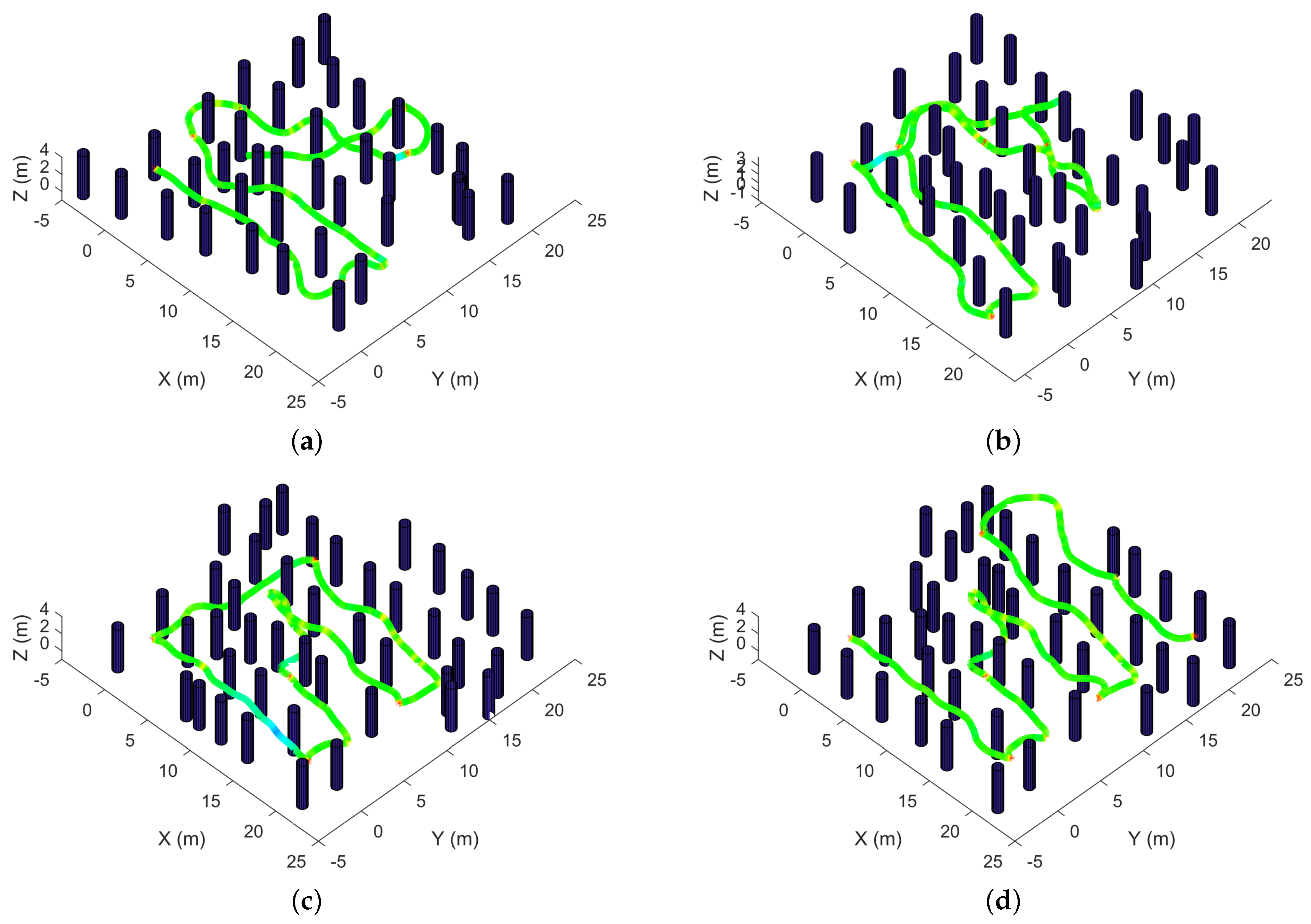
3.3. Simulation Environments

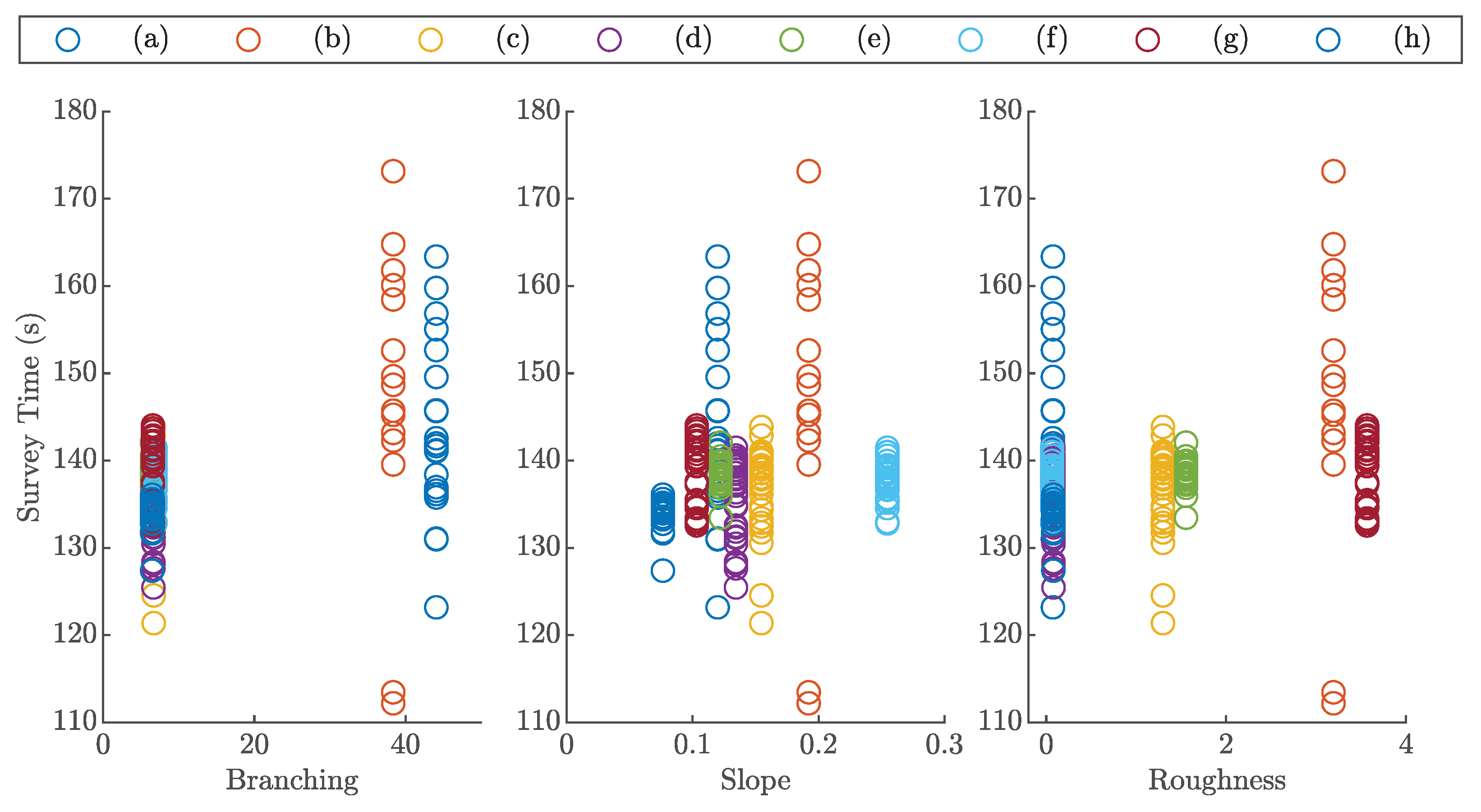
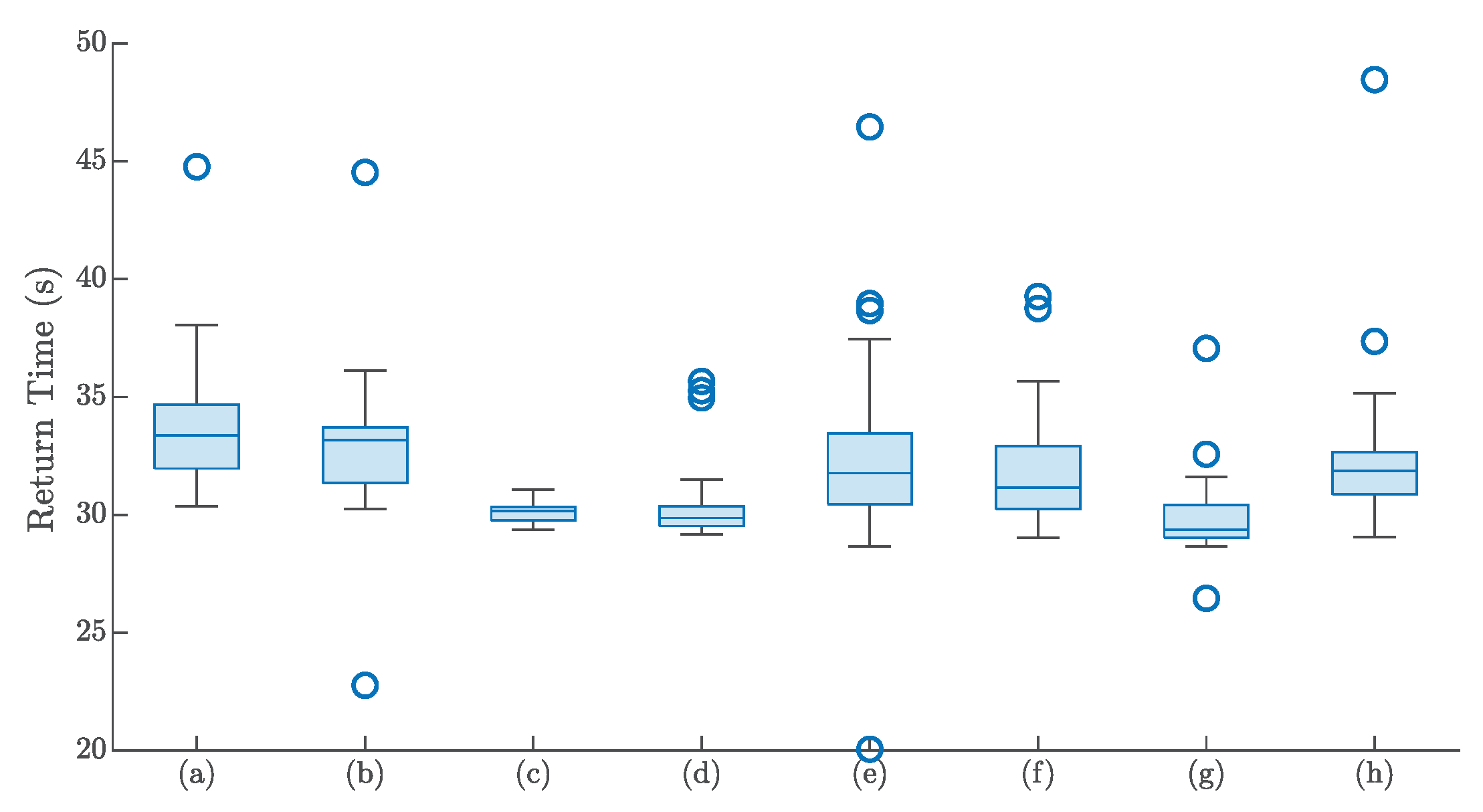
A set of eight simulation environments are selected from a large pool of generated environments, each representing a specific combination of difficulty metrics. These environments are shown in Figure 14, and the metrics describing each one is outlined in

Table 2. Summary of parameters of the generated forest environments shown in Figure 14.

Label	Branching	Roughness	Slope	Type
(a)	44.1	0.074	0.120	High Branching
(b)	38.4	3.19	0.192	Mixed Difficult
(c)	6.68	1.30	0.154	Mixed Medium
(d)	6.66	0.081	0.134	Medium Slope
(e)	6.45	1.55	0.122	Medium Roughness
(f)	6.91	0.065	0.255	High Slope
(g)	6.57	3.57	0.103	High Roughness
(h)	6.48	0.079	0.076	Baseline

. In particular, test case (h) is the baseline test case with low branching, slope, and roughness. Test cases (a), (d)–(g) are picked to examine the effects of branching, slope, and roughness alone, as each case is picked to minimize the other two difficulty metrics. Lastly, test cases (b) and (c) test the overall performance when subject to mixed test cases.

3.4. Survey Time

The first set of simulated tests is conducted to examine the effects on survey time of the proposed method against changes in the environment. In this series of experiments, the simulated UAV is initially placed between two rows and tasked to explore five corridors, with a traversal distance of 20 m down each corridor for an overall survey area of approx. 22 m by 22 m with a target survey speed of 1m/s. Once the traversal of the required number of corridors is complete, the UAV is tasked with returning to the starting location. To separate overhead effects from the UAV returning to the origin and traversal down the five corridors, the recorded time is split into the survey and return phases, which are timed separately. The time taken for the survey phase of each test environment is shown in Figure 15, the sensitivity of survey times to each difficulty metric is shown in Figure 16, and the return times are in Figure 17. To prevent samples that do not fully explore the environment from skewing the results with faster surveys, surveys that do not observe every tree are marked as failed and not included. The final survey results are tabulated in

Table 3. Summary of survey time for each test environment.

Label	Trails	Incomplete	Mean (s)	SD (s)	Min (s)	Max (s)
(a)	26	4	143	10.0	123	163
(b)	26	11	147	16.9	112	173
(c)	28	1	137	5.2	121	144
(d)	30	0	136	4.5	125	141
(e)	30	0	139	1.5	133	142
(f)	28	0	138	2.3	133	141
(g)	29	0	139	3.7	133	144
(h)	26	0	134	1.7	127	136
Theoretical Minimum *	-	0	120	0	120	-

.

Inspection of Figure 15 shows that aside from environments (a) and (b), the proposed method produces similar survey times, both in mean and spread for all other test environments. In particular, the worst performing environment (c) produces a 3.7% increase in mean survey time and an approx. 200% increase in standard deviation compared to the baseline environment (h). The mixed difficulty samples (a) and (b), however, produce noticeably higher mean and standard deviation increases of 6.7%/9.7% and 488%/894% respectively, with a corresponding increase in the number of incomplete surveys. Since environments (a) and (b) are the only ones with increased branching, this suggests that branching is the only parameter out of the three tests that affect traversal performance. Figure 16 supports this finding as there appears to be no visible correlation between survey time, slope, or roughness, and only a weak correlation with branching is seen. Little variation is seen in the return times outlined in Figure 17, with differences across operating environments likely arising from differences in the test scenes. This suggests that the proposed method is robust against various environmental conditions.

3.5. Coverage

The second important metric to evaluate for performance is the coverage of the environment, particularly the number of observed points corresponding to each tree. Thus, this series of experiments explores the sensitivity of coverage performance to varying environments for the proposed methods. Recorded data from the flights outlined in Section 3.4 are used to determine the number of points in a 1m by 1m square centered at the reference location of each tree. To eliminate run-to-run variation, the densities around each tree in the environment is averaged across all runs, providing the results shown in Figure 18 and

Table 4. Summary of coverage for each test environment.

Label	Mean (s)	SD (s)	Min (s)	Max (s)
(a)	2055	687	1099	3453
(b)	757	492	139	2218
(c)	1477	600	532	2629
(d)	1188	748	137	3551
(e)	1830	797	707	3894
(f)	1540	617	631	3044
(g)	1094	289	435	1500
(h)	1625	682	699	3400

. Figure 19 shows the distribution of coverage within each test environment. Points from the return portion of the flight are not included to avoid inflating coverage of trees observable from the return path.

Inspecting Table 4 shows two groups of mean coverages. The first of these groups consists of those with high mean points (>1400/stem) consisting of test environments (a), (c), (e), (f), and (h), and the second group consists of low mean points (<1200/stem) consisting of environments (b), (d), (g). Except for sample (d), both samples (b) and (g) consist of high-roughness environments. This suggests that this difference can be partially attributed to the limited LiDAR FOV, as rough terrain would likely result in more LiDAR points striking the ground within the FOV of any forward-facing inclines. This is supported by Figure 18, which shows a decrease in coverage with increasing roughness, but no clear correlation to the other two parameters.

All test environments appear to offer relatively even coverage when looking at Figure 19. Interestingly, however, the spread of coverage does not appear to be governed by roughness, as the high-roughness test case (g) offers the lowest standard deviation and visually the most consistent point density around each tree. Similarly, samples (b) and (d) appear to have a low point count but offer relatively similar coverage across all observed stems. Nevertheless, all trees within the environment have been observed at least once, suggesting that the proposed method generally produces good coverage across various test conditions.

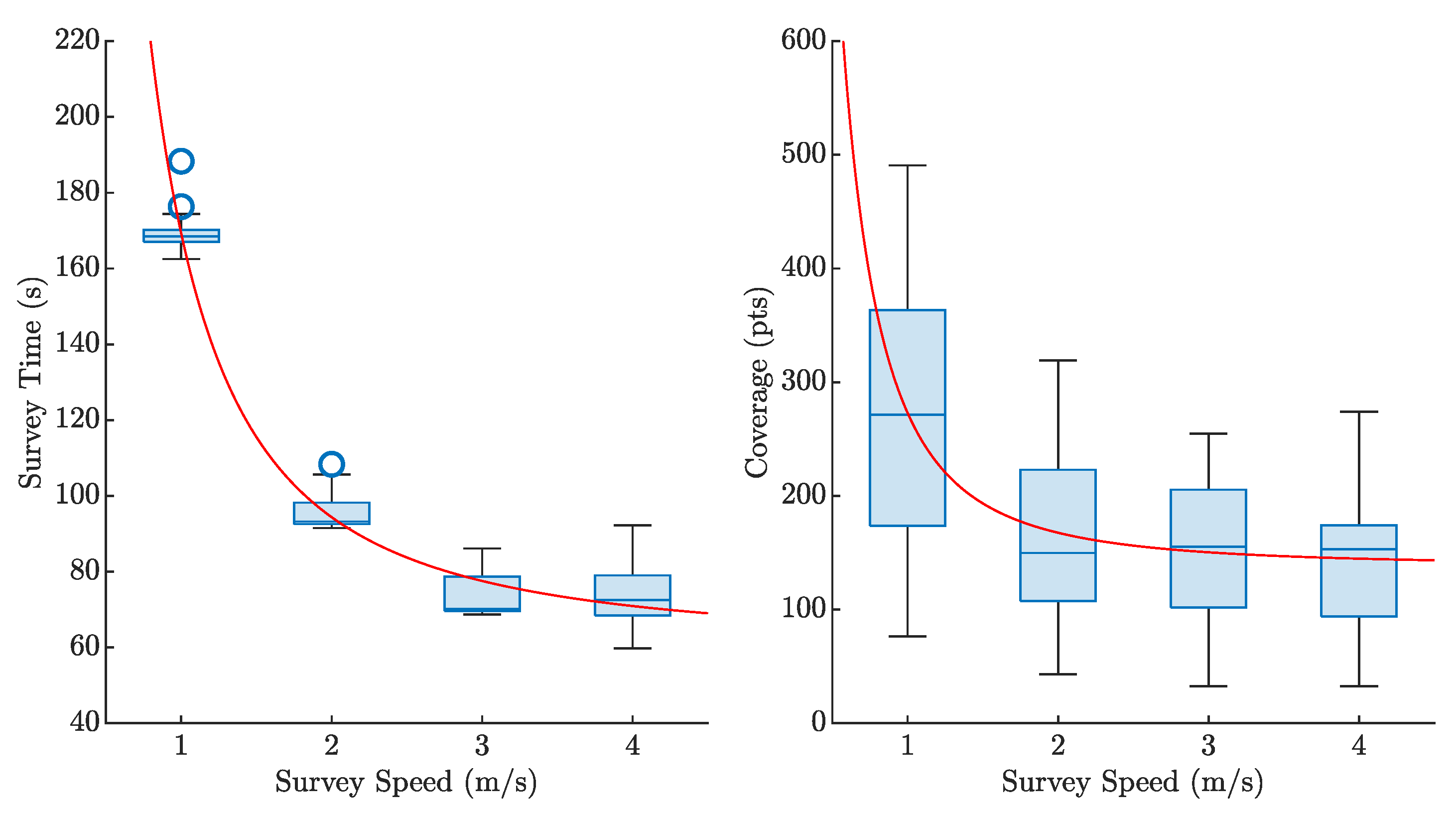
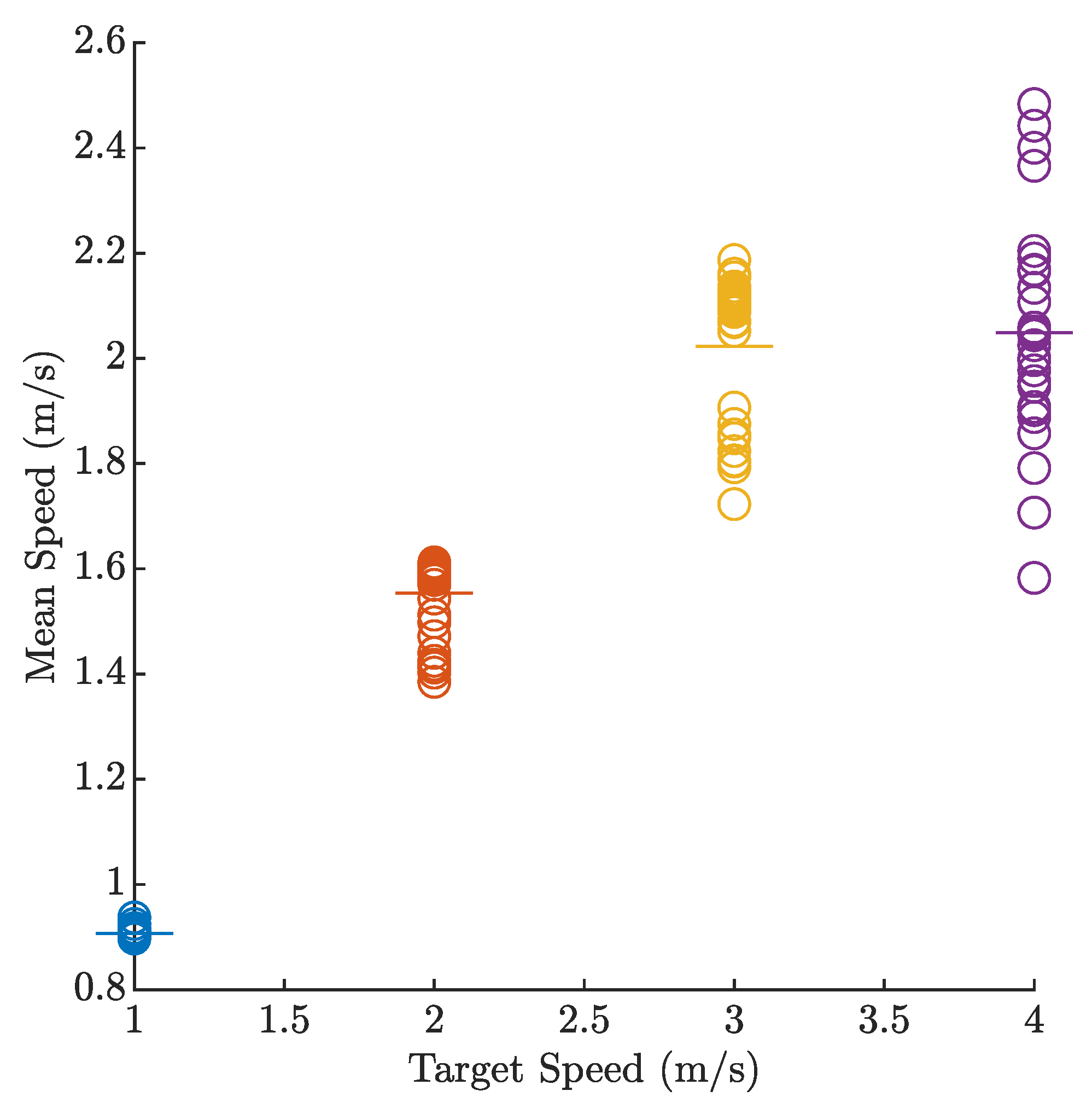
3.6. Effects of Survey Speed

As one of the planner’s objectives is to produce fixed-speed trajectories, an additional tuning factor is the target survey speed. In this series of tests, the proposed method is used on the baseline test environment (g) and tasked to explore the environment at target speeds between 1 m/s to 4 m/s in 1 m/s increments. Figure 20 shows the resulting survey time and tree coverages. Expectedly, survey time and coverage decrease logarithmically as the survey speed increases, with a decrease of 44% between target speeds of 1 m/s and 2 m/s, decreasing to 23% between 2 ms/ and 3 m/s, and no decrease between 3 m/s and 4 m/s. Environment coverage shows the same trend, with a reduction of approx. 39% between survey speeds of 1 m/s and 2 m/s, but no further noticeable decreases from speeds of 2 m/s and beyond.

Interestingly, the spread of survey times at a survey speed of 4 m/s is significantly higher when compared to at 3 m/s, with an increased spread of 88%. However, effects on the coverage appear to be relatively small at survey speeds above 2 m/s with little change in both coverage, mean, and spread. The increase in the spread and mean survey time between target speeds of 3 m/s and 4 m/s likely arises from the planner producing more unsafe trajectories from unobserved obstacles. This effect can be seen in Figure 21; the average speed of the survey does not increase at a target speed of 4 m/s compared to 3 m/s, but the spread of mean speeds is larger. In all cases, the actual mean speed is lower than the target speed, with the deficit increasing with increasing target speed.

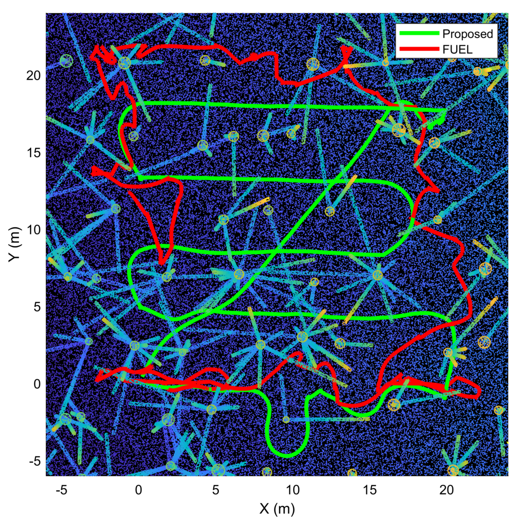
3.7. Comparison to Existing Methods

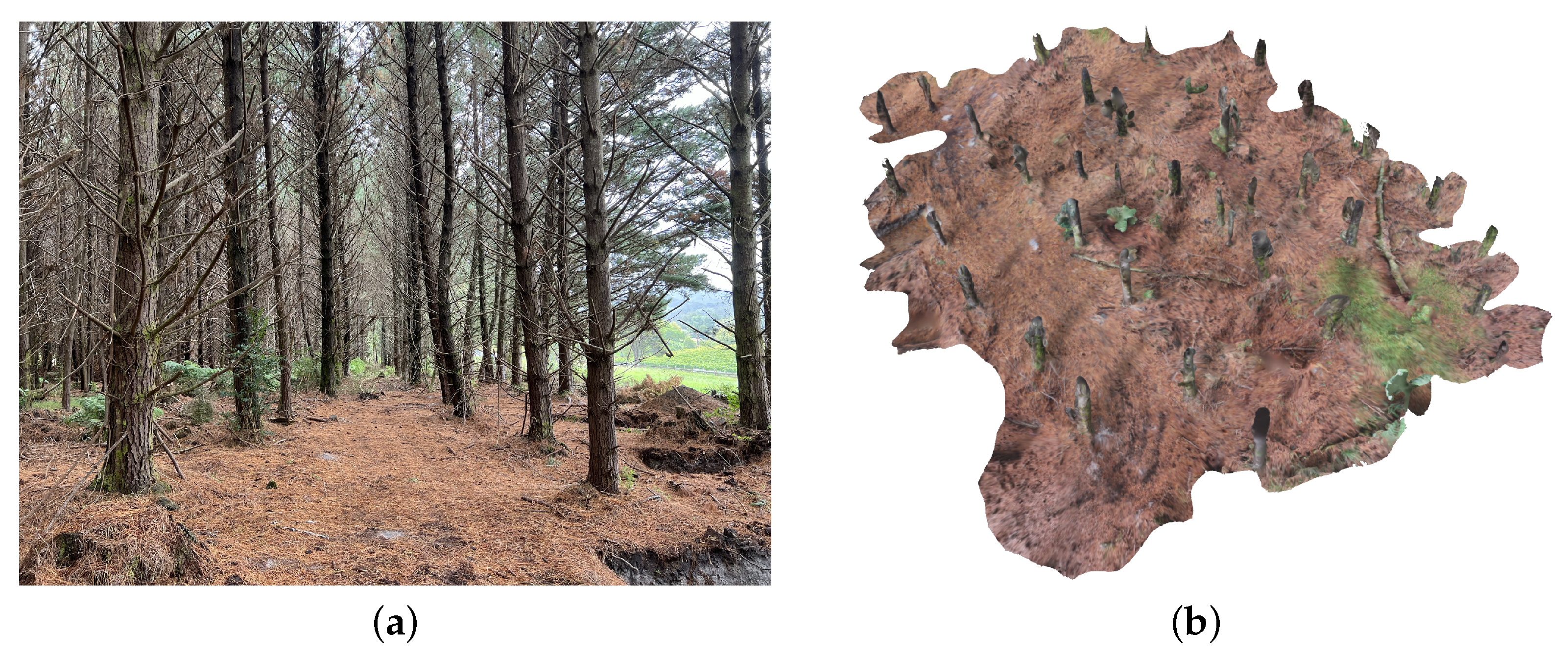
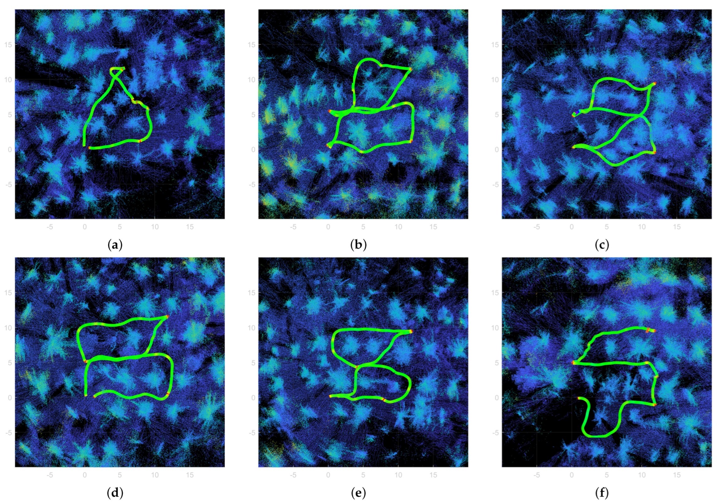
Finally, to examine the relative performance of the proposed method against other state-of-the-art exploration planners, an experiment is conducted using FUEL [28] to fully explore the same 22 m by 22 m area in environment (a) as the earlier trials. To ensure consistency between the two tests, the sensor model used in FUEL is updated to match that of the Livox MID-70, and the maximum velocity is limited to 1 m/s. Figure 22 shows the path taken within the environment for the two methods, with the proposed method completing the survey in 169 s, while FUEL took 306 s for completion. This disparity appears to be a result of FUEL needing to explicitly observe the entire environment, which results in a large amount of yaw action and traversal near the boundaries of the exploration volume as a result of the low FOV sensor. This manifests as a less consistent survey path shown in red in Figure 22. In contrast, the proposed method allows for longer straight sections, which allows the UAV to traverse at the target speed of 1 m/s for longer. This experiment demonstrates the performance advantage the proposed traversal method achieves against a high-performance generalized exploration method.

4. Flight Tests

Flight testing is performed at a local Pinus Radiata plantation to validate the proposed surveying method. The test site shown in Figure 23 is located in Riverhead Forest, Auckland, New Zealand (−36.725286, 174.547957) and consists of seven parallel rows spaced approximately 4.5 m apart with flat terrain. While there is little undergrowth in the environment, the environment is unpruned and contains many branches down to ground level. Despite branching, sufficient space exists between adjacent rows of trees to allow traversal down and between rows. The presence of trees in the middle of traversed rows produces some corridors which are not continuous.

Ten flights are conducted to evaluate the method, four of which are large-scale flights intending to cover the entire survey environment. The other six consists of small-scale flights covering smaller areas to test multiple different initial conditions. In addition to the survey and return times outlined previously, these trials also evaluate the number of attempted and completed corridors. These are defined as:

• Attempted corridors—the number of identified corridors and an attempt to traverse these corridors have been made
• Completed corridors—the number of correctly traversed corridors

4.1. Large Flights

Simplified views of the four flights are presented in Figure 24, and top-down views of the flight path overlaid on the reconstructed pointcloud for each flight is shown in Figure 25. Metrics summarizing the performance of each test flight is shown in

Table 5. Summary of large scale flight tests.

Label	Attempted	Completed	Survey Time (s)	Return Time (s)
(a)	3	2	114.5	-
(b)	4	3	135.5	25.5
(c)	4	4	106.4	18.7
(d)	5	5	157.8	-

. Of the four flights performed, tests (b) and (c) successfully returned to the origin, while (a) and (d) performed a partial and no return from the loss of the pose estimate. The UAV successfully selects waypoints and navigates between three to five corridors within the environment in all four cases. In particular, cases (a) and (b) show more complex routes around multiple trees rather than the mainly straight routes seen while traversing down a single corridor. This verifies the capability of the planner to produce safe trajectories with correctly placed waypoints when operating in a complex plantation environment.

Looking instead at the speed distribution along the survey path, the UAV maintains the target survey speed of 1 m/s throughout most traversal tests. A significant decrease in survey speed occurs at the last waypoint of each corridor, with smaller drops in regions with less free space and spaces with a large number of obstacles. The speed profile for the survey (d) shown in Figure 26 illustrates these events, with significant drops in survey speed occurring at approximately 30 s, 45 s, 80 s, and 120 s from the start of the survey and more minor fluctuations between these points. The large drops to near zero speed correspond with the end of each corridor and encompass the time taken to produce new waypoints in the neighboring corridor and generate a new trajectory. The smaller decreases in speed are likely caused by one of two things: FOV constraints reducing flight speed until the LiDAR is oriented in the correct direction, or trajectory splice events causing small local discontinuities in the trajectory. Overall, these experiments suggest that the proposed method can often correctly estimate the position of the rows of trees, and the trajectory planner and follower can successfully generate and execute safe trajectories for the survey. However, there is room for improvement of efficiency through optimizing regions with slow survey speed.

4.2. Small Flights

Since the size of the test plot is limited, a set of six small flights through the environment is conducted to examine the robustness of the proposed method against different initial conditions. A random starting point with sufficient adjacent rows to complete the survey is selected for each trial. In each task, the UAV uses the proposed method to traverse approx. 12 m down each corridor, with the complete survey consisting of three corridors. The total survey area for each of the trails is approx. 14 m by 14 m. Top-down views of each flight within the reconstructed point cloud are shown in Figure 27, and a performance summary is outlined in

Table 6. Summary of small scale flight tests.

Label	Attempted	Completed	Survey Time (s)	Return Time (s)
(a)	3	3	49.8	15.3
(b)	3	3	66.7	20.4
(c)	3	3	61.8	20.2
(d)	3	3	62.9	23.1
(e)	3	3	52.6	20.4
(f)	3	3	69.7	-

.

All flights successfully traversed the target area, providing complete coverage of the trees within the approx. 14 m by 14 m bounding square. In particular, test cases (a), (c), and (f) consist of initial conditions where the UAV is unable to traverse down every corridor in a straight path continuously, and safe trajectories are generated and executed in each case. Aside from (f), all tests produced and executed a safe return trajectory. Furthermore, experiments (a), (c), and (f) demonstrate initial conditions where straight line traversal is not possible due to obstacles present. In all cases, the planner successfully determined a safe trajectory to navigate around these obstacles and complete the survey. These flight experiments demonstrate the robustness of the proposed method against varying conditions and untraversable regions within the scene.

5. Conclusions

This paper presents a system for autonomous exploration of plantation forests using multi-rotor UAVs. First, a method for navigation waypoint generation using estimated tree row positions from occupancy data is presented. Next, a non-linear optimization-based approach is proposed to generate smooth, constant velocity survey trajectories using B-Splines and an ESDF map to create dynamically feasible and collision-free trajectories in complex environments. Lastly, an MPC trajectory tracker is implemented to follow the generated trajectories. Simulation testing is performed using eight procedurally generated forests replicating spacing information from real plantation forests, completing 22 m by 22 m surveys in approx. 140 s. These results demonstrate the proposed method’s ability to operate in various environments and initial conditions. Lastly, four large-scale and six small-scale flight tests are successfully performed within a local plantation forest, demonstrating our proposed method’s correct row identification, waypoint placement, and navigation capabilities.

The results of this research pave the way for fully autonomous navigation in plantation forests, with potential extension into other row-based environments such as orchards or vineyards. While this study explores the autonomous navigation problem during the survey aspect, the current iteration of the system still requires manual traversal to reach the starting point of the survey. Therefore, future work could consist of investigations into long-range traversal methods allowing for arbitrary starting positions, i.e., from outside of the forest. Furthermore, alternative methods for waypoint generation and/or row segmentation could be explored for additional survey speeds or accuracy. Finally, other navigation methods such as machine-learning-based end-to-end approaches could be explored for potential performance gains in this application.

References

1. Deadman, M.W.; Goulding, C.J. A method for assessment of recoverable volume by log types. N. Z. J. For. Sci. 1979, 9, 225–239. [Google Scholar]
2. Interpine Innovation. PlotSafe Overlapping Feature Crusing Forest Inventory Procedures; Interpine Innovation: Rotorua, New Zealand, 2007; p. 49. [Google Scholar]
3. Hudak, A.T.; Crookston, N.L.; Evans, J.S.; Hall, D.E.; Falkowski, M.J. Nearest neighbor imputation of species-level, plot-scale forest structure attributes from LiDAR data. Remote Sens. Environ. 2008, 112, 2232–2245. [Google Scholar] [CrossRef]
4. Puliti, S.; Dash, J.P.; Watt, M.S.; Breidenbach, J.; Pearse, G.D. A comparison of UAV laser scanning, photogrammetry and airborne laser scanning for precision inventory of small-forest properties. For. Int. J. For. Res. 2020, 93, 150–162. [Google Scholar] [CrossRef]
5. Mielcarek, M.; Kamińska, A.; Stereńczak, K. Digital Aerial Photogrammetry (DAP) and Airborne Laser Scanning (ALS) as Sources of Information about Tree Height: Comparisons of the Accuracy of Remote Sensing Methods for Tree Height Estimation. Remote Sens. 2020, 12, 1808. [Google Scholar] [CrossRef]
6. Bauwens, S.; Bartholomeus, H.; Calders, K.; Lejeune, P. Forest inventory with terrestrial LiDAR: A comparison of static and hand-held mobile laser scanning. Forests 2016, 7, 127. [Google Scholar] [CrossRef]
7. Kukko, A.; Kaijaluoto, R.; Kaartinen, H.; Lehtola, V.V.; Jaakkola, A.; Hyyppä, J. Graph SLAM correction for single scanner MLS forest data under boreal forest canopy. ISPRS J. Photogramm. Remote Sens. 2017, 132, 199–209. [Google Scholar] [CrossRef]
8. Wang, Y.; Kukko, A.; Hyyppä, E.; Hakala, T.; Pyörälä, J.; Lehtomäki, M.; El Issaoui, A.; Yu, X.; Kaartinen, H.; Liang, X.; et al. Seamless integration of above- and under-canopy unmanned aerial vehicle laser scanning for forest investigation. For. Ecosyst. 2021, 8, 10. [Google Scholar] [CrossRef]
9. Hyyppä, E.; Hyyppä, J.; Hakala, T.; Kukko, A.; Wulder, M.A.; White, J.C.; Pyörälä, J.; Yu, X.; Wang, Y.; Virtanen, J.P.; et al. Under-canopy UAV laser scanning for accurate forest field measurements. ISPRS J. Photogramm. Remote Sens. 2020, 164, 41–60. [Google Scholar] [CrossRef]
10. Hyyppä, J.; Yu, X.; Hakala, T.; Kaartinen, H.; Kukko, A.; Hyyti, H.; Muhojoki, J.; Hyyppä, E. Under-Canopy UAV Laser Scanning Providing Canopy Height and Stem Volume Accurately. Forests 2021, 12, 856. [Google Scholar] [CrossRef]
11. Del Perugia, B.; Krisanski, S.; Taskhiri, M.S.; Turner, P. Below-canopy UAS photogrammetry for stem measurement in radiata pine plantation. Proc. Remote Sens. Agric. Ecosyst. Hydrol. 2018, 11, 1078309. [Google Scholar] [CrossRef]
12. Krisanski, S.; Taskhiri, M.S.; Turner, P. Enhancing Methods for Under-Canopy Unmanned Aircraft System Based Photogrammetry in Complex Forests for Tree Diameter Measurement. Remote Sens. 2020, 12, 1652. [Google Scholar] [CrossRef]
13. Kuželka, K.; Surový, P. Mapping Forest Structure Using UAS inside Flight Capabilities. Sensors 2018, 18, 2245. [Google Scholar] [CrossRef] [PubMed]
14. Jiang, S. Towards Autonomous Flights of an Unmanned Aerial Vehicle (UAV) in Plantation Forests. Master’s Thesis, The University of Auckland, Auckland, New Zealand, 2016. [Google Scholar]
15. Chiella, A.C.B.; Machado, H.N.; Teixeira, B.O.S.; Pereira, G.A.S. GNSS/LiDAR-Based Navigation of an Aerial Robot in Sparse Forests. Sensors 2019, 19, 4061. [Google Scholar] [CrossRef]
16. Chisholm, R.A.; Cui, J.; Lum, S.K.Y.; Chen, B.M. UAV LiDAR for below-canopy forest surveys. J. Unmanned Veh. Syst. 2013, 1, 61–68. [Google Scholar] [CrossRef]
17. Cui, J.Q.; Lai, S.; Dong, X.; Liu, P.; Chen, B.M.; Lee, T.H. Autonomous navigation of UAV in forest. In Proceedings of the 2014 International Conference on Unmanned Aircraft Systems, ICUAS 2014—Conference Proceedings, Orlando, FL, USA, 27–30 May 2014. [Google Scholar] [CrossRef]
18. Thrun, S.; Montemerlo, M. The graph SLAM algorithm with applications to large-scale mapping of urban structures. Int. J. Robot. Res. 2006, 25, 403–429. [Google Scholar] [CrossRef]
19. Zucker, M.; Ratliff, N.; Dragan, A.D.; Pivtoraiko, M.; Klingensmith, M.; Dellin, C.M.; Bagnell, J.A.; Srinivasa, S.S. CHOMP: Covariant Hamiltonian optimization for motion planning. Int. J. Robot. Res. 2013, 32, 1164–1193. [Google Scholar] [CrossRef]
20. Oleynikova, H.; Burri, M.; Taylor, Z.; Nieto, J.; Siegwart, R.; Galceran, E. Continuous-time trajectory optimization for online UAV replanning. In Proceedings of the IEEE International Conference on Intelligent Robots and Systems 2016, Daejeon, Korea, 9–14 October 2016; pp. 5332–5339. [Google Scholar] [CrossRef]
21. Usenko, V.; Von Stumberg, L.; Pangercic, A.; Cremers, D. Real-time trajectory replanning for MAVs using uniform B-splines and a 3D circular buffer. In Proceedings of the IEEE International Conference on Intelligent Robots and Systems, Vancouver, BC, Canada, 24–28 September 2017; pp. 215–222. [Google Scholar] [CrossRef]
22. Zhou, B.; Pan, J.; Gao, F.; Shen, S. RAPTOR: Robust and Perception-Aware Trajectory Replanning for Quadrotor Fast Flight. IEEE Trans. Robot. 2021, 37, 1992–2009. [Google Scholar] [CrossRef]
23. Mellinger, D.; Kumar, V. Minimum snap trajectory generation and control for quadrotors. In Proceedings of the IEEE International Conference on Robotics and Automation, Shanghai, China, 9–13 May 2011; pp. 2520–2525. [Google Scholar] [CrossRef]
24. Tordesillas, J.; Lopez, B.T.; How, J.P. FASTER: Fast and Safe Trajectory Planner for Flights in Unknown Environments. In Proceedings of the 2019 IEEE/RSJ International Conference on Intelligent Robots and Systems (IROS), Macau, China, 3–8 November 2019; pp. 1934–1940. [Google Scholar] [CrossRef]
25. Deits, R.; Tedrake, R. Efficient mixed-integer planning for UAVs in cluttered environments. In Proceedings of the IEEE International Conference on Robotics and Automation, Seattle, WA, USA, 26–30 May 2015; pp. 42–49. [Google Scholar] [CrossRef]
26. Gao, F.; Wang, L.; Zhou, B.; Zhou, X.; Pan, J.; Shen, S. Teach-Repeat-Replan: A Complete and Robust System for Aggressive Flight in Complex Environments. IEEE Trans. Robot. 2020, 36, 1526–1545. [Google Scholar] [CrossRef]
27. Meng, Z.; Qin, H.; Chen, Z.; Chen, X.; Sun, H.; Lin, F.; Ang, M.H. A Two-Stage Optimized Next-View Planning Framework for 3-D Unknown Environment Exploration, and Structural Reconstruction. IEEE Robot. Autom. Lett. 2017, 2, 1680–1687. [Google Scholar] [CrossRef]
28. Zhou, B.; Zhang, Y.; Chen, X.; Shen, S. FUEL: Fast UAV Exploration using Incremental Frontier Structure and Hierarchical Planning. IEEE Robot. Autom. Lett. 2021, 6, 779–786. [Google Scholar] [CrossRef]
29. Dharmadhikari, M.; Dang, T.; Solanka, L.; Loje, J.; Nguyen, H.; Khedekar, N.; Alexis, K. Motion Primitives-based Path Planning for Fast and Agile Exploration using Aerial Robots. In Proceedings of the 2020 IEEE International Conference on Robotics and Automation (ICRA), Paris, France, 31 May–31 August 2020; pp. 179–185. [Google Scholar] [CrossRef]
30. Bircher, A.; Kamel, M.; Alexis, K.; Oleynikova, H.; Siegwart, R. Receding Horizon “Next-Best-View” Planner for 3D Exploration. In Proceedings of the 2016 IEEE International Conference on Robotics and Automation (ICRA), Stockholm, Sweden, 16–21 May 2016; pp. 1462–1468. [Google Scholar] [CrossRef]
31. Schmid, L.; Pantic, M.; Khanna, R.; Ott, L.; Siegwart, R.; Nieto, J. An Efficient Sampling-Based Method for Online Informative Path Planning in Unknown Environments. IEEE Robot. Autom. Lett. 2020, 5, 1500–1507. [Google Scholar] [CrossRef]
32. Papachristos, C.; Khattak, S.; Alexis, K. Uncertainty-aware receding horizon exploration and mapping using aerial robots. In Proceedings of the 2017 IEEE International Conference on Robotics and Automation (ICRA), Singapore, 29 May–3 June 2017; pp. 4568–4575. [Google Scholar] [CrossRef]
33. Xu, Z.; Deng, D.; Shimada, K. Autonomous UAV Exploration of Dynamic Environments Via Incremental Sampling and Probabilistic Roadmap. IEEE Robot. Autom. Lett. 2021, 6, 2729–2736. [Google Scholar] [CrossRef]
34. Lin, T.J.; Stol, K.A. Faster Navigation of Semi-Structured Forest Environments using Multi-Rotor UAVs. Robotica 2022. submitted. [Google Scholar]
35. Stanford Artificial Intelligence Laboratory. Robotic Operating System. Available online: https://www.ros.org (accessed on 15 June 2022).
36. Lin, J.; Zhang, F. R3LIVE: A Robust, Real-Time, RGB-Colored, LiDAR-Inertial-Visual Tightly-Coupled State Estimation and Mapping Package. In Proceedings of the 2022 International Conference on Robotics and Automation (ICRA), Philadelphia, PA, USA, 23–27 May 2022; pp. 10672–10678. [Google Scholar] [CrossRef]
37. Zhang, W.; Qi, J.; Peng, W.; Wang, H.; Xie, D.; Wang, X.; Yan, G. An Easy-to-Use Airborne LiDAR Data Filtering Method Based on Cloth Simulation. Remote Sens. 2016, 8, 501. [Google Scholar] [CrossRef]
38. Ester, M.; Kriegel, H.P.; Sander, J.; Xu, X. A Density-Based Algorithm for Discovering Clusters in Large Spatial Databases with Noise; AAAI Press: Palo Alto, CA, USA, 1996; pp. 226–231. [Google Scholar]
39. Han, L.; Gao, F.; Zhou, B.; Shen, S. FIESTA: Fast Incremental Euclidean Distance Fields for Online Motion Planning of Aerial Robots. In Proceedings of the IEEE International Conference on Intelligent Robots and Systems, Macau, China, 3–8 November 2019; pp. 4423–4430. [Google Scholar] [CrossRef]
40. Hart, P.E.; Nilsson, N.J.; Raphael, B. A Formal Basis for the Heuristic Determination of Minimum Cost Paths. IEEE Trans. Syst. Sci. Cybern. 1968, 4, 100–107. [Google Scholar] [CrossRef]
41. Agarwal, S.; Mierle, K.; Team, T.C.S. Ceres Solver. Available online: https://github.com/ceres-solver/ceres-solver (accessed on 15 June 2022).
42. Lin, T.J.; Stol, K.A. Fast Trajectory Tracking of Multi-Rotor UAVs using First-Order Model Predictive Control. In Proceedings of the 2021 Australian Conference on Robotics and Automation (ACRA), Melbourne, Australia, 6–8 December 2021. [Google Scholar]
43. Houska, B.; Ferreau, H.J.; Diehl, M. ACADO toolkit—An open-source framework for automatic control and dynamic optimization. Optim. Control Appl. Methods 2011, 32, 298–312. [Google Scholar] [CrossRef]
44. Perlin, K. An Image Synthesizer. In Proceedings of the SIGGRAPH ’85: 12th Annual Conference on Computer Graphics and Interactive Techniques, San Francisco, CA, USA, 22–26 July 1985; Association for Computing Machinery: New York, NY, USA, 1985; pp. 287–296. [Google Scholar] [CrossRef]
Figure 1. Examples of plantation forests which are (a) traversable, and (b) untraversable on foot in Kaingaroa Forest, Rotorua, New Zealand. Note the presence of an available flight corridor in both environments.
Drones 06 00256 g001
Figure 2. UAV used for flight testing. The carried payload consists of a Livox MID-70 LiDAR, Intel Realsense T265, and an Intel NUC. The body and inertial frames are denoted as { B } and { I } respectively.
Drones 06 00256 g002
Figure 3. Overall task flow during the survey process. Pose estimation and mapping are not within the scope of this work.
Drones 06 00256 g003
Figure 4. Horizontal slice of a point cloud in a typical New Zealand plantation forest with rows labeled. Note the lack of consistent structure in the orthogonal direction.
Drones 06 00256 g004
Figure 5. Approximate survey plan consisting of a lawnmowing pattern aligned with plantation rows.
Drones 06 00256 g005
Figure 6. Top-down views of (a) good, and (b) poor alignment between { I X } and the principle row directions of the plantation forest.
Drones 06 00256 g006
Figure 7. Sample environment consisting of two rows with r , θ labeled. The dotted yellow line denotes the traversable corridor.
Drones 06 00256 g007
Figure 8. Overall trajectory planner pipeline.
Drones 06 00256 g008
Figure 9. Worst case B-Spline collision scenario with degree 3. The trajectory is guaranteed to be collision-free if the three convex hulls shown in blue, orange, and green are obstacle free.
Drones 06 00256 g009
Figure 10. Top down view of a typical replanning event, showing the elements of a newly observed obstacle and a splice event.
Drones 06 00256 g010
Figure 11. Simplified version of the forward paths of the cascaded multi-rotor controller with unified and airframe-specific portions highlighted.
Drones 06 00256 g011
Figure 12. Proposed controller structure.
Drones 06 00256 g012
Figure 13. Illustration of parameters modeled in Table 1.
Drones 06 00256 g013
Figure 14. Simulation test environments. The three numbers in the subfigure captions correspond to the branching, roughness, and slope metrics.
Drones 06 00256 g014
Figure 15. Summary of survey time for each test environment. Trials that did not produce full coverage are not included. Circles denote outliers in the survey time.
Drones 06 00256 g015
Figure 16. Effects on survey time with varying test environments.
Drones 06 00256 g016
Figure 17. Summary of return times for each test environment with incomplete trials removed.
Drones 06 00256 g017
Figure 18. Effects on coverage when the three test parameters are varied.
Drones 06 00256 g018
Figure 19. Averaged coverage maps for trials in environments (ah), normalized to the maximum of each specific sample. Blue hues indicate trees with fewer observed points, and green hues indicate more observed points. Non-uniformity is shown as the difference in hues.
Drones 06 00256 g019
Figure 20. Effects on survey time (left) and coverage (right) with varying speed. Exponential fit through all results is shown as a red line.
Drones 06 00256 g020
Figure 21. Plot of mean speed vs. target survey speed. Note the plateau in mean speed at 3 m/s and 4 m/s. The averaged mean speed across all samples for each target speed is indicated by a horizontal line.
Drones 06 00256 g021
Figure 22. Path taken for complete coverage for the proposed method and FUEL.
Drones 06 00256 g022
Figure 23. (a) Single row view of the plantation site used for flight testing, note the presence of some low-hanging branches, and (b) 3D scan of the proposed test site showing the survey region; the scan area is approx. 25 m by 30 m.
Drones 06 00256 g023
Figure 24. Simplified views of the large-scale test flights (ad), the path followed is shown as a solid line overlaid with stem locations within the environment. Greener hues indicate a flight speed closer to the 1 m/s target speed, while red hues indicate slower speeds taken.
Drones 06 00256 g024
Figure 25. Top-down views of large-scale test flights (ad), with the path taken overlaid on the reconstructed point cloud.
Drones 06 00256 g025
Figure 26. Plot of estimated speed during trial (d).
Drones 06 00256 g026
Figure 27. Top-down views of path taken during small-scale test flights (af) overlaid on the reconstructed point clouds. The path taken during the survey is shown as the line.
Drones 06 00256 g027