
Automated Sortie Scheduling Optimization for Fixed-Wing Unmanned Carrier Aircraft and Unmanned Carrier Helicopter Mixed Fleet Based on Offshore Platform


Abstract
1. Introduction
2. Related Works
2.1. Fleet Sortie Scheduling
2.2. Hybrid Flow Shop Problem
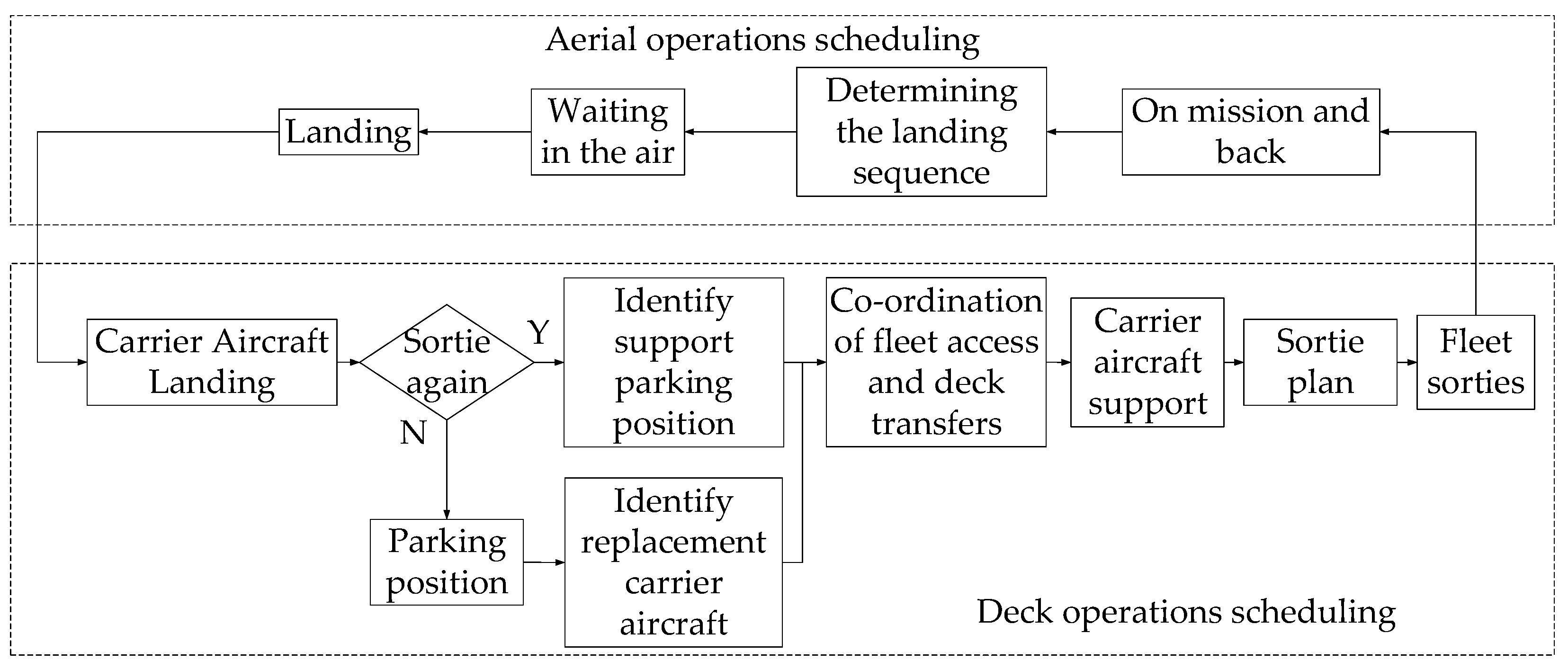
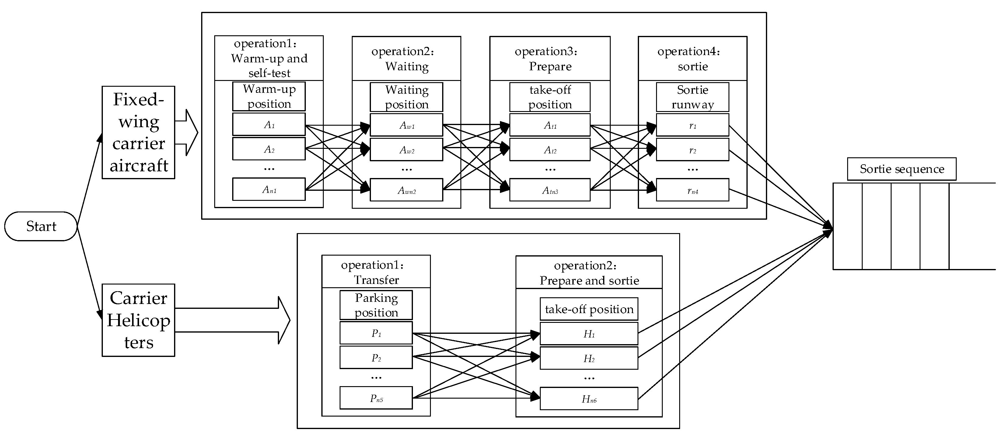
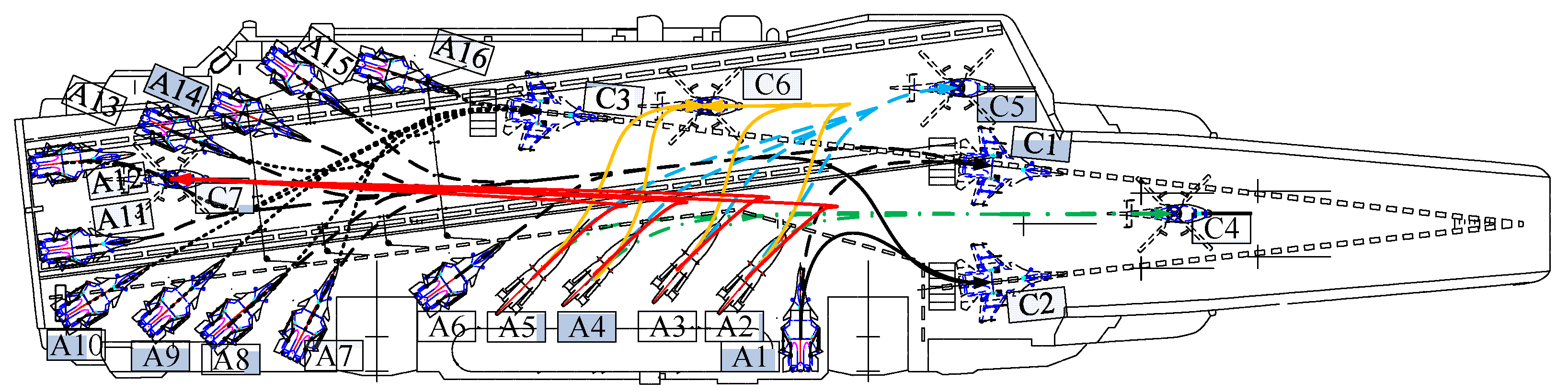
3. Description of the Problem
- Warm-up and self-test. According to the requirements of fixed-wing carrier engines, a warm-up and self-test are required before take-off, to confirm whether the performance indicators of the engine are normal. This stage generally requires 2–3 min. Because of the design characteristics of the carrier structure, some positions cannot operate aircraft warm-ups, as the fixed-wing aircraft tail flames would cause ablation of the carrier structure: therefore, some aircraft need to be transferred at this stage.
- Waiting behind the deflector. When the aircraft completes the engine warm-up and self-test, it is transferred to the take-off position. If the target take-off position already exists, the aircraft will be transferred to the waiting position behind the target take-off position: as this stage involves deck transit, transit collision avoidance constraints must be considered, to prevent collisions due to interference in the path of the carrier aircraft.
- Preparation at the take-off position. Once the aircraft has reached the target take-off position, it can be prepared for take-off.
- Take-off. When the carrier aircraft has completed all preparations, it waits for the take-off order, and completes it.
- Transfer to take-off position. After the helicopter has completed its support, it can be transferred to the target take-off position: this stage requires consideration of the transit path blocking, aircraft position interference, and transit collision avoidance constraints. The road conditions determine the timing of the helicopter transfer, and the helicopter must wait in the original parking position when there is a helicopter in the target position.
- Take-off preparation and take-off. Once the helicopter has reached the target take-off position, preparations are made for take-off, such as rotor deployment, navigation calibration, and control system self-testing. After completing this series of tasks, the helicopter can wait for the take-off command to execute the take-off, which takes approximately 5 min.
- Warm-up position constraints. As mentioned above, a fixed-wing aircraft needs to be transferred first, for aircraft that are unable to complete engine warm-up in their initial position. The transfer must be operated when no warm-up position is available, after the other aircraft has left the parking position.
- Transport collision avoidance restraints, to ensure that no collisions occur during the carrier aircraft transfer process.
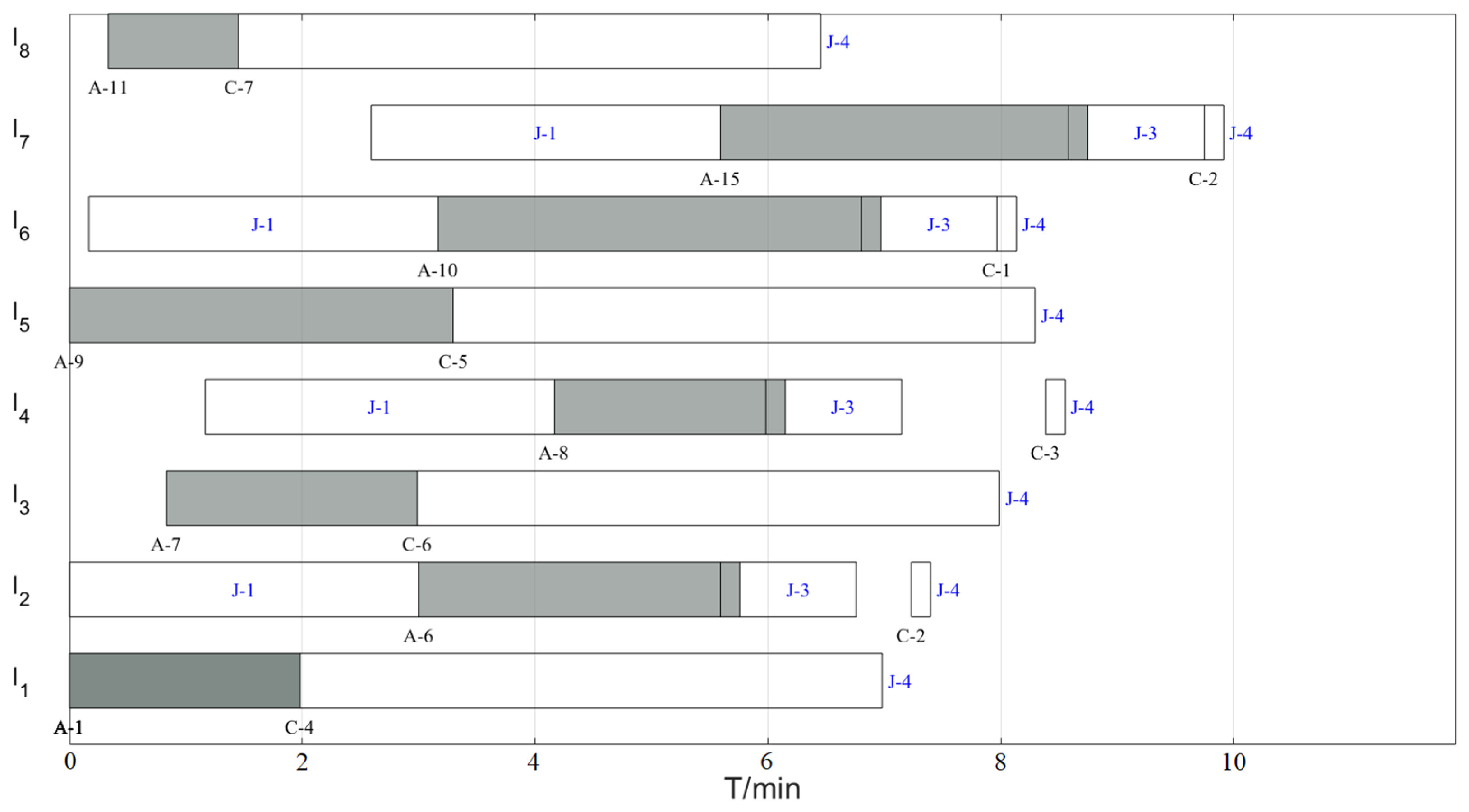
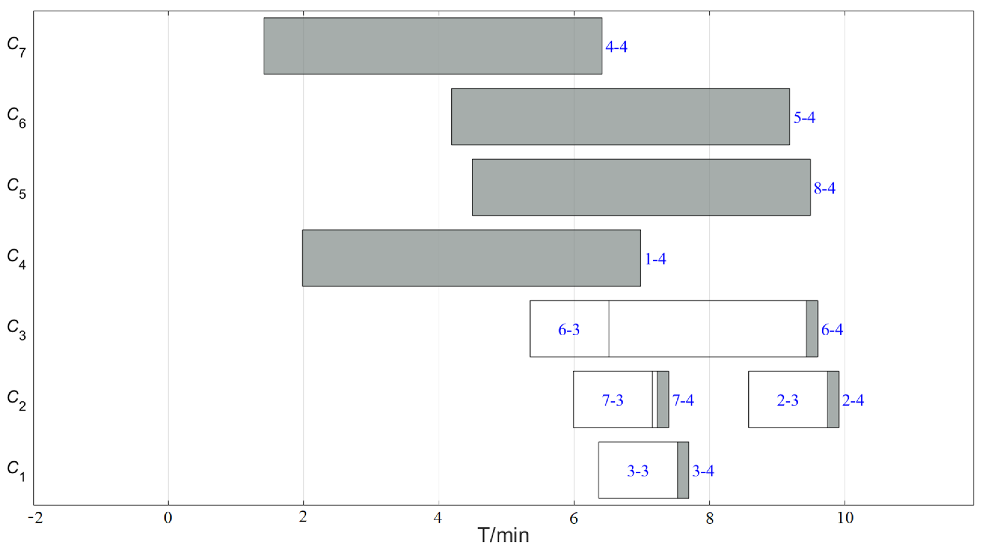
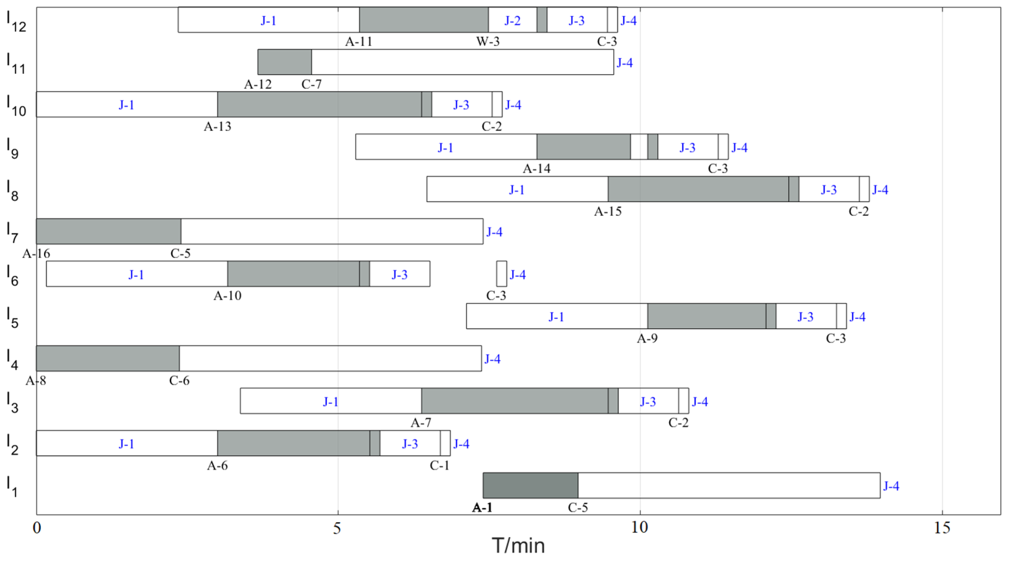
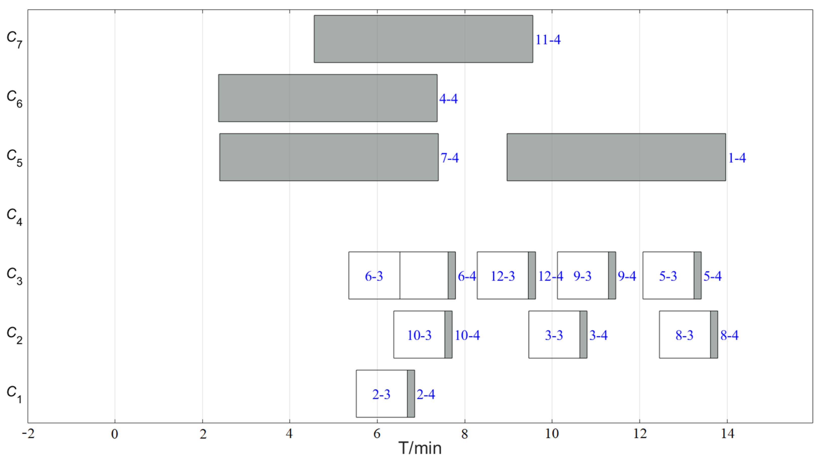
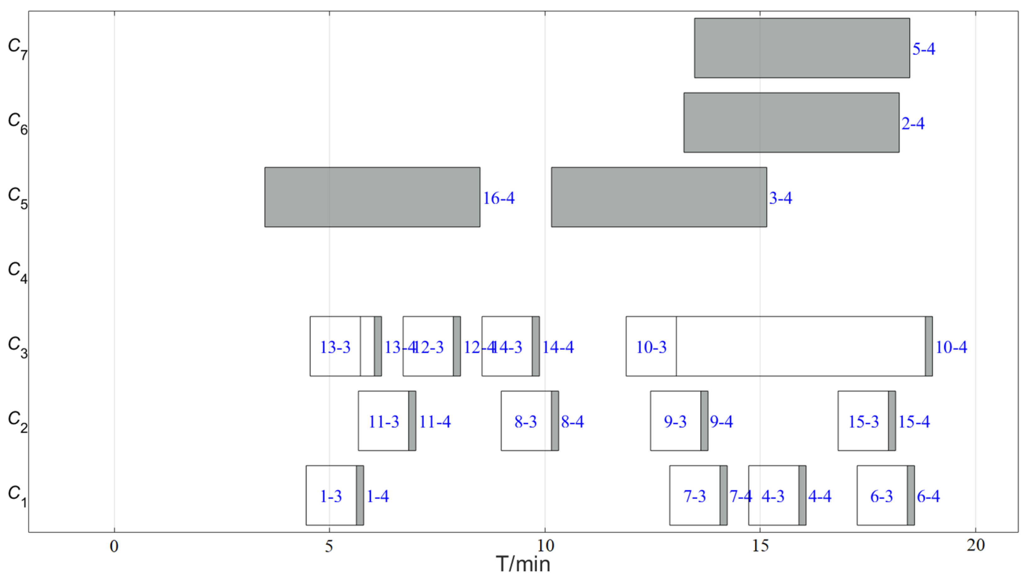
- Blockage of transit path by parking position. As shown in Figure 3, for helicopter take-off position C7, all helicopters selecting the C7 take-off position will interfere with the carrier aircraft A12, A13, and A14. Only after the A12, A13, and A14 carrier aircraft take off will the taxi to take-off position for C7 be clear.
- Runway incursion constraint. As shown in Figure 3, if a carrier aircraft is parked at the C1 take-off position or the waiting position behind it, it will invade the take-off runway of the C3 take-off position, which will cause C3 to be unable to take off. Similarly, the carrier helicopters parked at the C4 take-off position occupy the runways corresponding to the C1, C2, and C3 take-off positions, and the carrier helicopters parked at the C6 take-off position occupy the runway corresponding to the C3 take-off position.
- Take-off interval constraint. After a fixed-wing carrier aircraft takes off, its take-off wake disturbs the airflow field on the carrier surface, which leads to a higher risk for subsequent aircraft take-off, and the deflector plate behind the fixed-wing carrier aircraft take-off position also needs to be reset and cooled. For helicopters, it takes time to reach a safe distance from the carrier after take-off; therefore, after a carrier aircraft has taken off, a period of time must be allowed for the next carrier aircraft to take off, to ensure safe sortie.
- Operational flow constraint. Fixed-wing aircraft and carrier helicopters are required to complete their respective take-off procedures in a specific sequence before they can sortie.
- Take-off weight constraint. When the take-off weight of the carrier aircraft exceeds a certain limit, the take-off must be performed at the C3 take-off position with a longer glide distance, to ensure that the carrier aircraft achieves the required speed when leaving the deck.
- Take-off position selection constraint. As fixed-wing aircraft and helicopters have different types of take-off positions, they need to be constrained in the selection of take-off positions.
4. Path Library and Mathematical Formulation
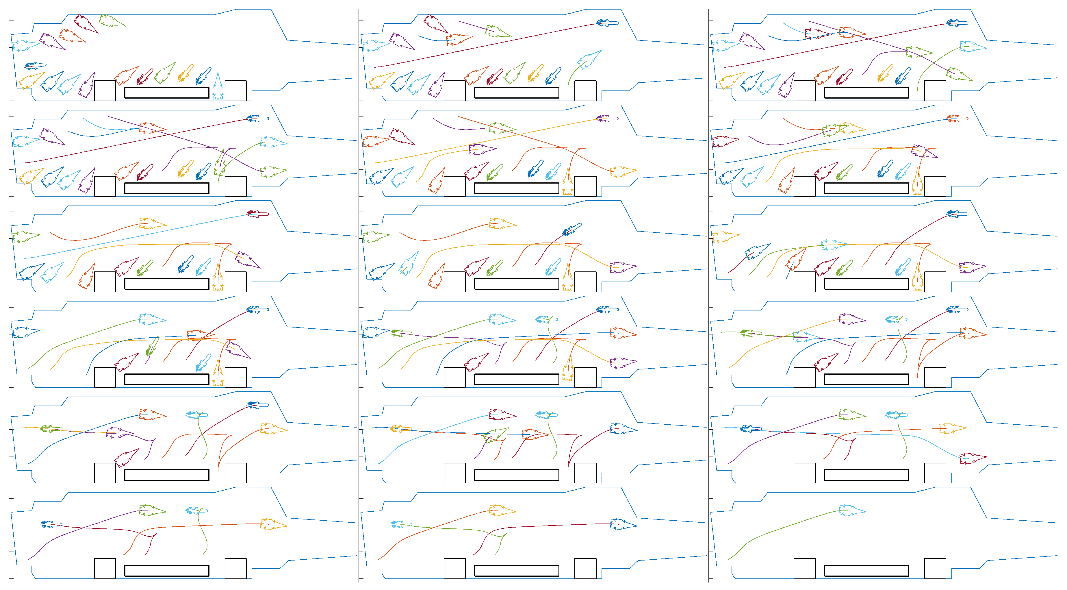
4.1. Path Library Construction
4.2. Mathematical Formulation
4.2.1. Problem Assumptions
- When an operation begins, it cannot be stopped;
- Only one transfer equipment may be accepted for transfer at any transfer stage at any one time;
- The carrier aircraft can perform a transfer operation with any transfer equipment corresponding to each stage;
- The parameters of the path library are constant, and are unaffected by other transfer operations;
- The interference of unexpected factors, such as malfunction, is not considered.
4.2.2. Notation
4.2.3. Optimization Objectives
- 6.
- Minimize fleet sortie completion time
- 7.
- Minimize fleet transit time
4.2.4. ASPMF Constraints
- 8.
- Timing constraint on workflow
- 9.
- Space resource constraint
- 10.
- Take-off position matching constraint
- 11.
- Take-off interval constraint
- 12.
- Take-off weight constraint
- 13.
- Decision variable constraint
- 14.
- Take-off position selection constraint
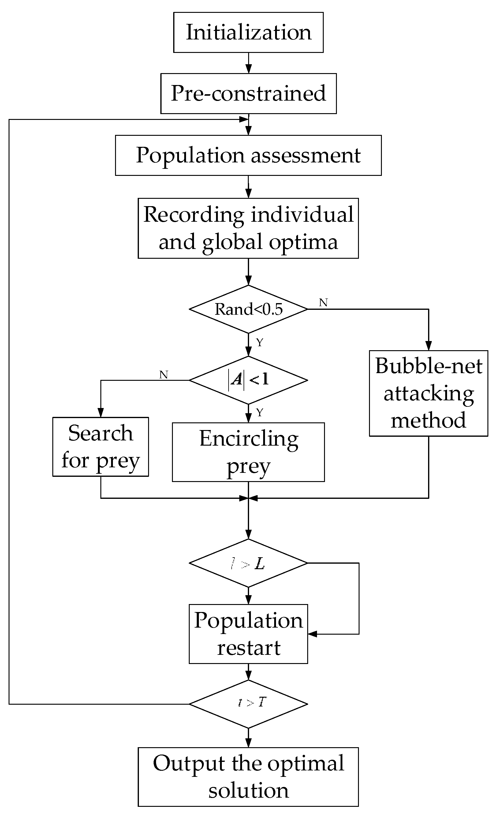
5. IWOA
5.1. The Principle of the WOA
5.2. Encoding and Decoding
5.3. Learning Factor
5.4. Discrete Design
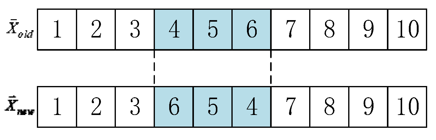
5.4.1. New Encircling Prey
5.4.2. New Bubble-Net Attacking Method
5.4.3. New Search for Prey
5.5. Pre-Constrained
5.6. Parameter Improvements
5.7. Population Restart
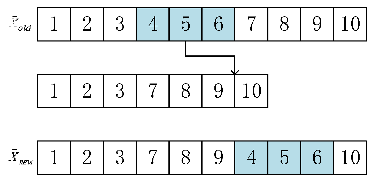
- Field reinsertion operations
- 2.
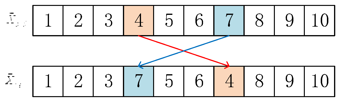
- Two-point crossover operations
- 3.
- Field inverse order operations
5.8. IWOA Processes
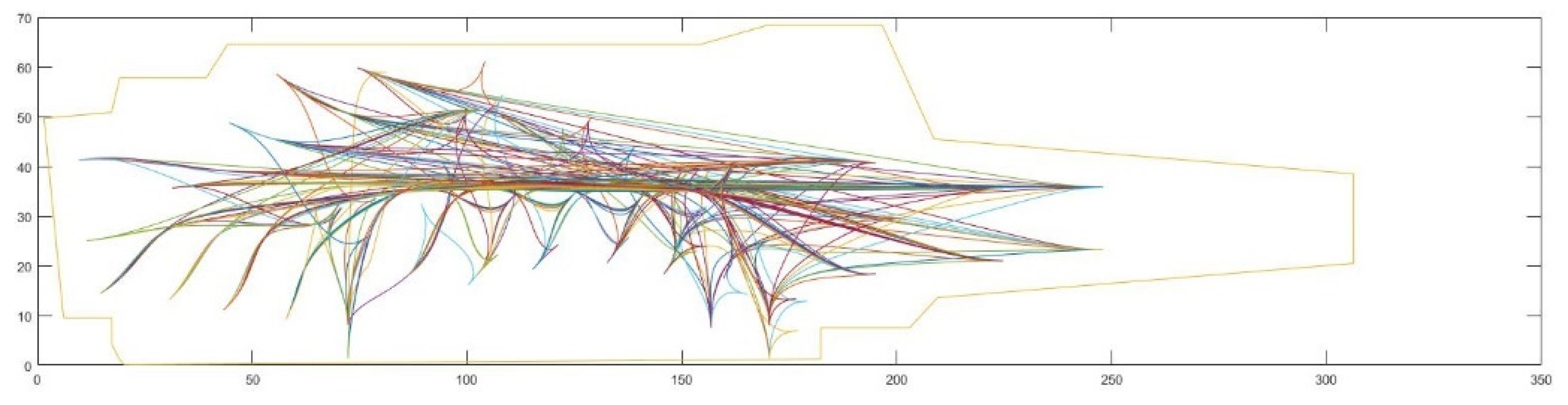
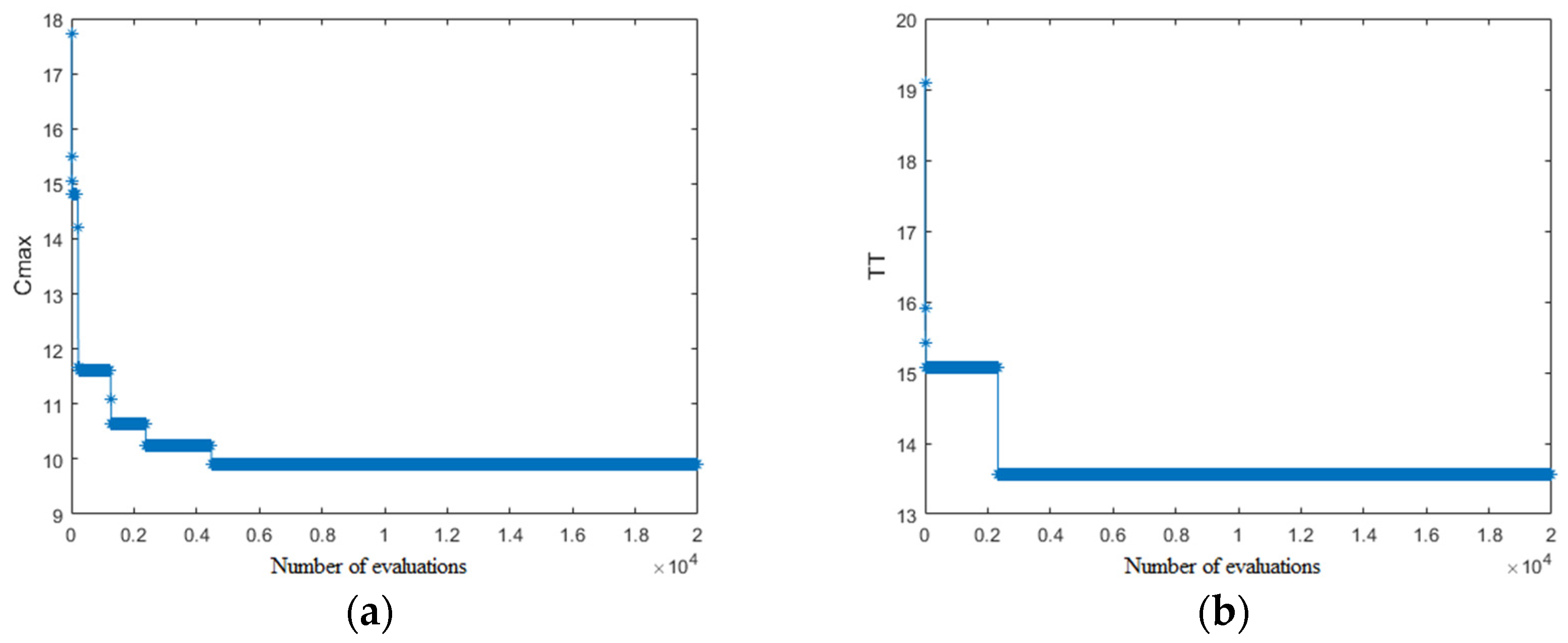
6. Case Study
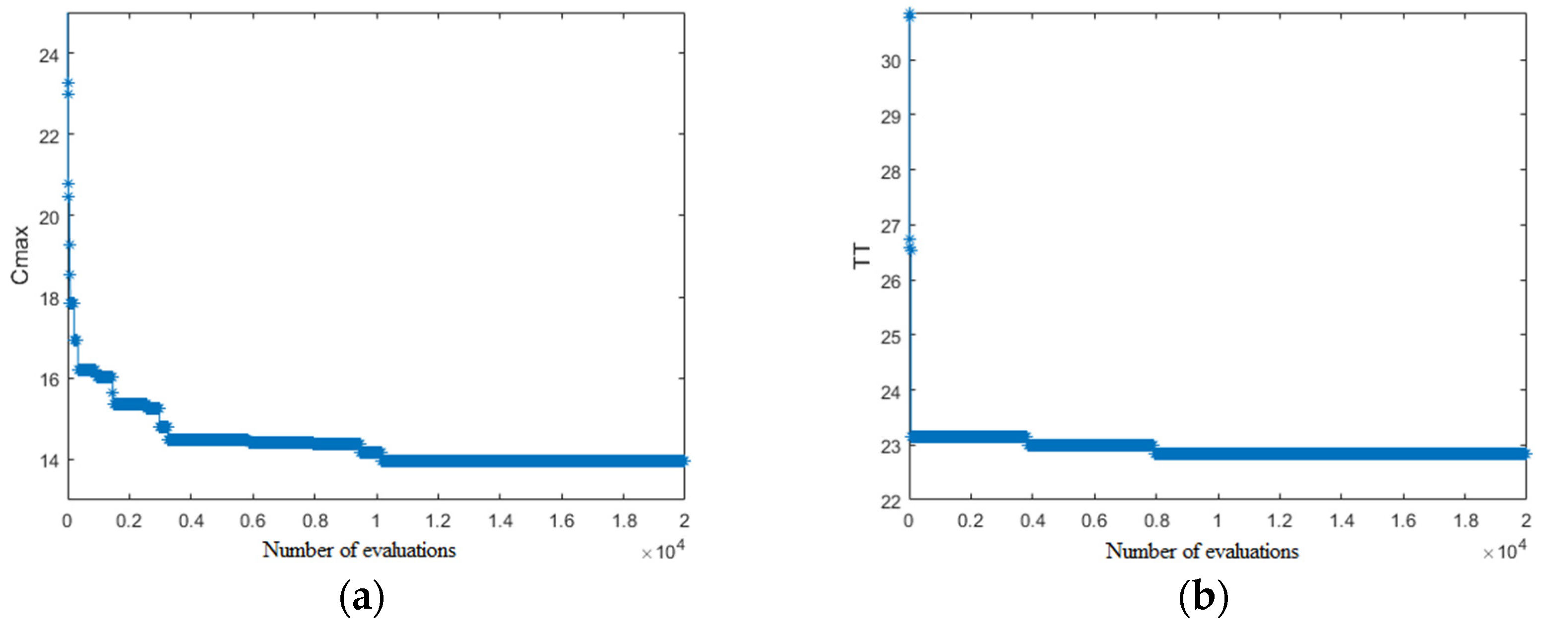
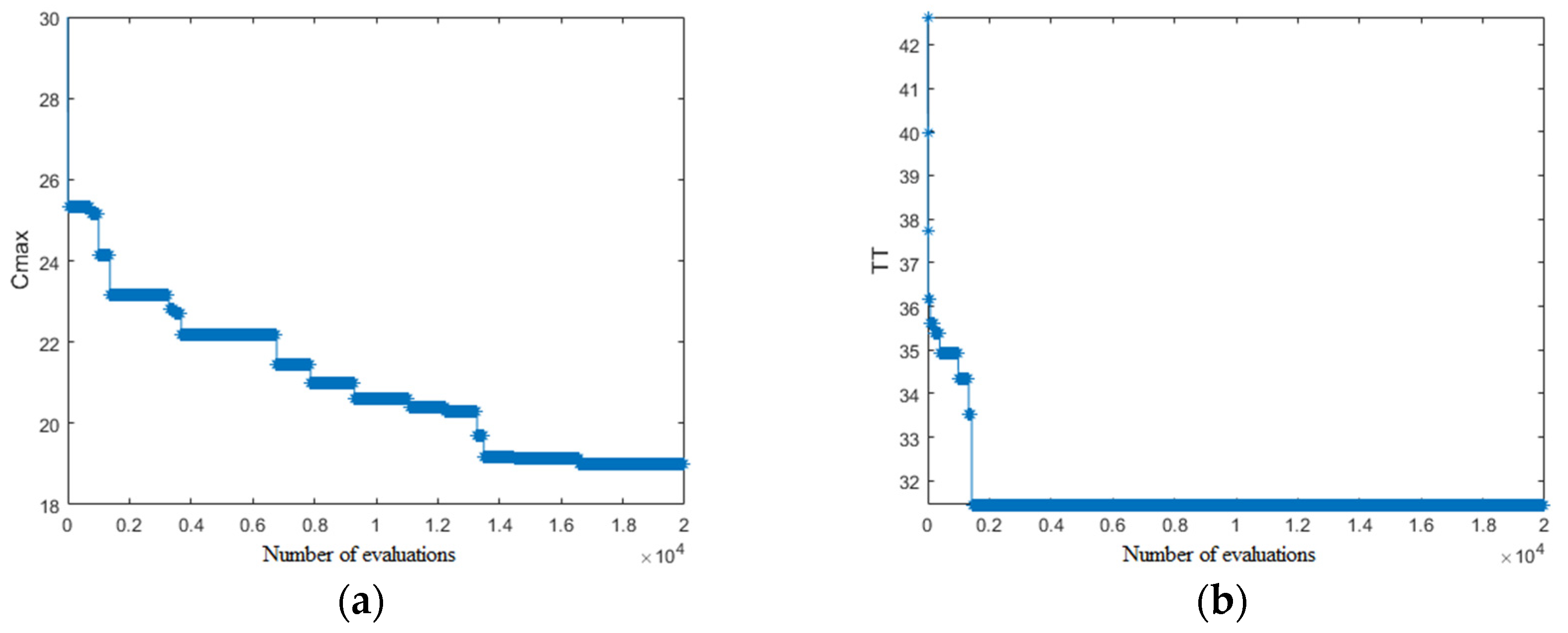
6.1. Orthogonal Optimization of Algorithm Parameters
6.2. Simulation of Different Sortie Cases
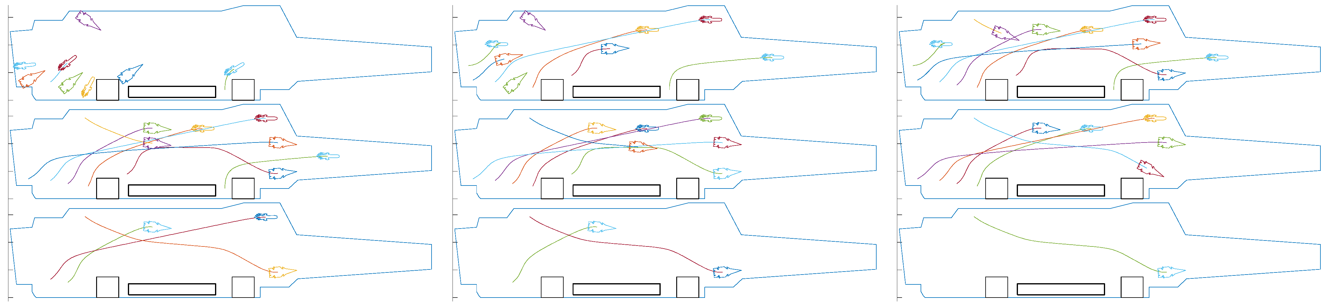
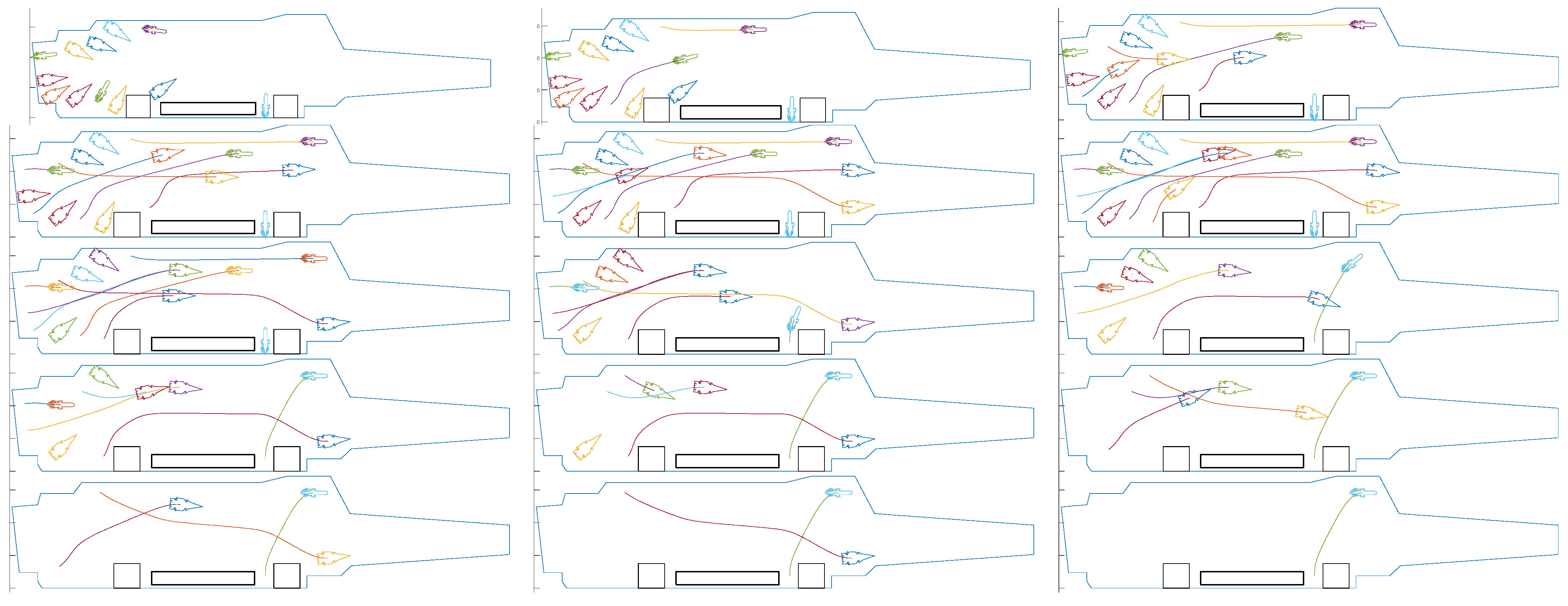
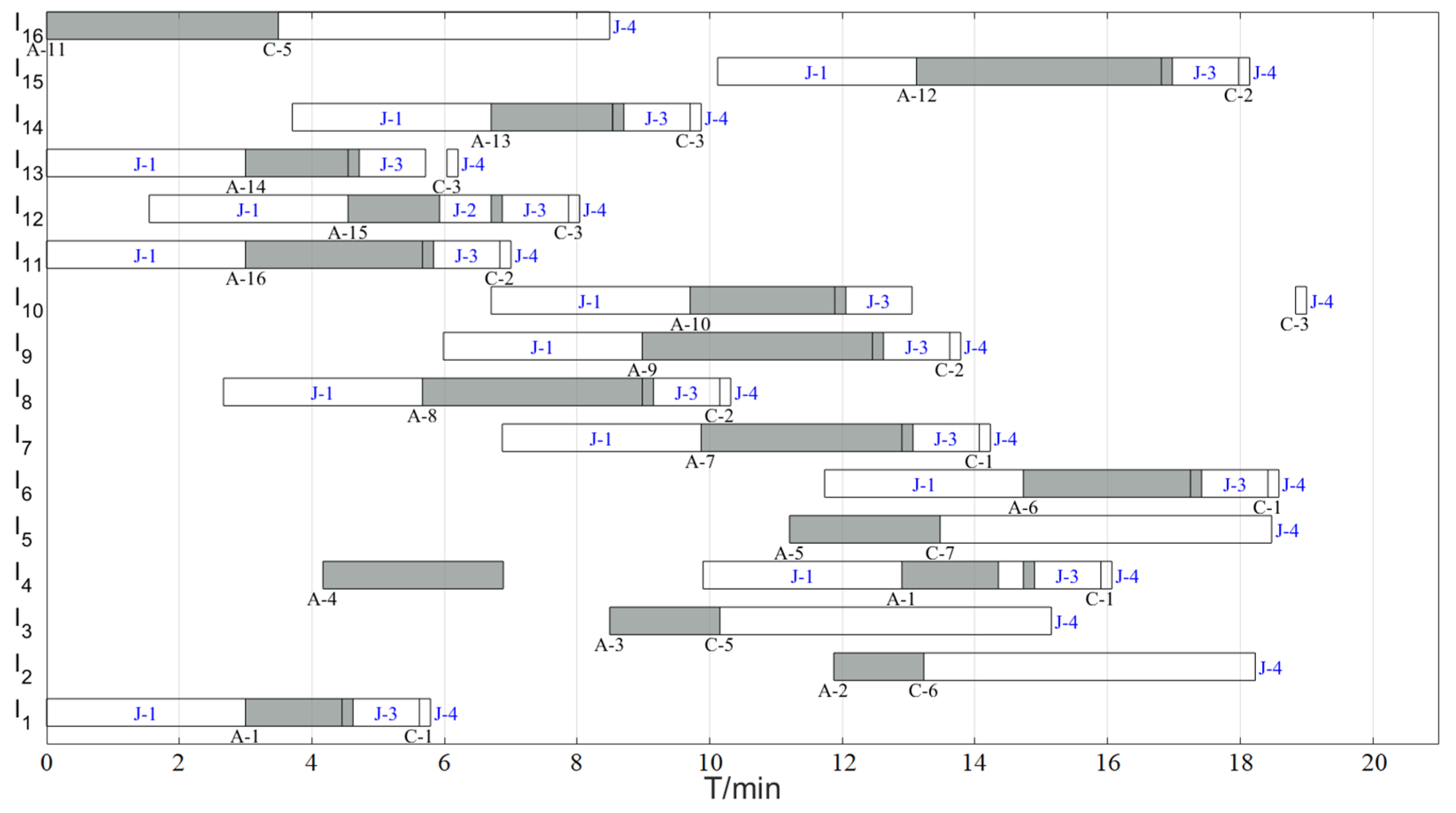
6.2.1. 8-Aircraft Sortie Case
6.2.2. 12-Aircraft Sortie Case
6.2.3. 16-Aircraft Sortie Case
6.3. Comparison of Different Sortie Strategies
7. Conclusions
Author Contributions
Funding
Institutional Review Board Statement
Informed Consent Statement
Data Availability Statement
Conflicts of Interest
References
- Michini, B.; How, J. A Human-Interactive Course of Action Planner for Aircraft Carrier Deck Operations. In Proceedings of the Infotech@Aerospace 2011, St. Louis, MO, USA, 29–31 March 2011; American Institute of Aeronautics and Astronautics: St. Louis, MO, USA, 2011. [Google Scholar]
- Ryan, J.; Cummings, M.; Roy, N.; Banerjee, A.; Schulte, A. Designing an Interactive Local and Global Decision Support System for Aircraft Carrier Deck Scheduling. In Proceedings of the Infotech@Aerospace 2011, St. Louis, MO, USA, 29–31 March 2011; American Institute of Aeronautics and Astronautics: St. Louis, MO, USA, 2011. [Google Scholar]
- Ryan, J.C.; Banerjee, A.G.; Cummings, M.L.; Roy, N. Comparing the Performance of Expert User Heuristics and an Integer Linear Program in Aircraft Carrier Deck Operations. IEEE Trans. Cybern. 2014, 44, 761–773. [Google Scholar] [CrossRef] [PubMed]
- Ryan, J.C.; Cummings, M.L. Assessing the Performance of Human-Automation Collaborative Planning Systems. Ph.D. Thesis, Massachusetts Institute of Technology, Cambridge, MA, USA, 2011. [Google Scholar]
- Cui, R.; Han, W.; Su, X.; Zhang, Y.; Guo, F. A multi-objective hyper heuristic framework for integrated optimization of carrier-based aircraft flight deck operations scheduling and resource configuration. Aerosp. Sci. Technol. 2020, 107, 106346. [Google Scholar] [CrossRef]
- Yuan, P.; Han, W.; Su, X.; Liu, J.; Song, J. A Dynamic Scheduling Method for Carrier Aircraft Support Operation under Uncertain Conditions Based on Rolling Horizon Strategy. Appl. Sci. 2018, 8, 1546. [Google Scholar] [CrossRef]
- Zheng, M.; Yang, F.; Dong, Z.; Xie, S.; Chu, X. Carrier-borne aircrafts aviation operation automated scheduling using multiplicative weights apprenticeship learning. Int. J. Adv. Robot. Syst. 2019, 16, 1729881419828917. [Google Scholar] [CrossRef]
- Liu, J.; Han, W.; Peng, H.; Wang, X. Trajectory planning and tracking control for towed carrier aircraft system. Aerosp. Sci. Technol. 2019, 84, 830–838. [Google Scholar] [CrossRef]
- Wu, Y.; Sun, L.; Qu, X. A sequencing model for a team of aircraft landing on the carrier. Aerosp. Sci. Technol. 2016, 54, 72–87. [Google Scholar] [CrossRef]
- Wu, Y.; Wang, Y.; Qu, X.; Sun, L. Exploring mission planning method for a team of carrier aircraft launching. Chin. J. Aeronaut. 2019, 32, 1256–1267. [Google Scholar] [CrossRef]
- Guo, F.; Han, W.; Su, X.; Liu, Y.; Cui, R. A bi-population immune algorithm for weapon transportation support scheduling problem with pickup and delivery on aircraft carrier deck. Def. Technol. 2021, S2214914721002282. [Google Scholar] [CrossRef]
- Yuan, Y.; Xu, H. Multiobjective Flexible Job Shop Scheduling Using Memetic Algorithms. IEEE Trans. Autom. Sci. Eng. 2015, 12, 336–353. [Google Scholar] [CrossRef]
- Driss, I.; Mouss, K.N.; Laggoun, A. A new genetic algorithm for flexible job-shop scheduling problems. J. Mech. Sci. Technol. 2015, 29, 1273–1281. [Google Scholar] [CrossRef]
- Liu, J.; Han, W.; Liu, C.; Peng, H. A New Method for the Optimal Control Problem of Path Planning for Unmanned Ground Systems. IEEE Access 2018, 6, 33251–33260. [Google Scholar] [CrossRef]
- Han, W.; Liu, Z.; Su, X.; Cui, K.; Liu, J. Deck path planning of carrier-based aircraft based on heuristic and optimal control. Syst. Eng. Electron. 2022, 1, 1–16. Available online: https://kns.cnki.net/kcms/detail/11.2422.TN.20220507.1357.002.html (accessed on 26 October 2022).
- Mirjalili, S.; Lewis, A. The Whale Optimization Algorithm. Adv. Eng. Softw. 2016, 95, 51–67. [Google Scholar] [CrossRef]
- Su, X.; Han, W.; Wu, Y.; Zhang, Y.; Liu, J. A Proactive Robust Scheduling Method for Aircraft Carrier Flight Deck Operations with Stochastic Durations. Complexity 2018, 2018, 6932985. [Google Scholar] [CrossRef]
- Liu, Y.; Han, W.; Su, X.; Cui, R. Optimization, of fixed aviation support resource station configuration for aircraft carrier based on aircraft dispatch mission scheduling. Chin. J. Aeronaut. 2022; in press. [Google Scholar] [CrossRef]
- Hu, H.; Wu, Y.; Xu, J.; Sun, Q. Path Planning for Autonomous Landing of Helicopter on the Aircraft Carrier. Mathematics 2018, 6, 178. [Google Scholar] [CrossRef]
- Su, X.; Li, Z.; Song, J.; Wang, L. A Path Planning Method for Carrier Aircraft on Deck Combining Artificial Experience and Intelligent Search. IOP Conf. Ser. Mater. Sci. Eng. 2018, 381, 12194. [Google Scholar] [CrossRef]
- Zhenxing, Y.; Ziyu, Y.; Wenhao, W.; Yichen, C.; Huiyuan, C. The enemy air-threat prediction based aircraft real-time path planning for offshore combat. In Proceedings of the 2018 IEEE 8th International Conference on Underwater System Technology: Theory and Applications (USYS), Wuhan, China, 1–3 December 2018; pp. 1–4. [Google Scholar]
- Si, W.; Sun, T.; Song, C.; Zhang, J. Design and verification of a transfer path optimization method for an aircraft on the aircraft carrier flight deck. Front. Inf. Technol. Electron. Eng. 2021, 22, 1221–1233. [Google Scholar] [CrossRef]
- Komaki, G.M.; Sheikh, S.; Malakooti, B. Flow shop scheduling problems with assembly operations: A review and new trends. Int. J. Prod. Res. 2019, 57, 2926–2955. [Google Scholar] [CrossRef]
- Ben-Yehoshua, Y.; Mosheiov, G. A single machine scheduling problem to minimize total early work. Comput. Oper. Res. 2016, 73, 115–118. [Google Scholar] [CrossRef]
- Yoo, J.; Lee, I.S. Parallel machine scheduling with maintenance activities. Comput. Ind. Eng. 2016, 101, 361–371. [Google Scholar] [CrossRef]
- Çaliş, B.; Bulkan, S. A research survey: Review of AI solution strategies of job shop scheduling problem. J. Intell. Manuf. 2015, 26, 961–973. [Google Scholar] [CrossRef]
- Shen, L.; Dauzère-Pérès, S.; Neufeld, J.S. Solving the flexible job shop scheduling problem with sequence-dependent setup times. Eur. J. Oper. Res. 2018, 265, 503–516. [Google Scholar] [CrossRef]
- Literature Review of Open Shop Scheduling Problems. Available online: https://www.scirp.org/html/4-8701327_53605.htm (accessed on 18 June 2022).
- Lin, S.-W.; Cheng, C.-Y.; Pourhejazy, P.; Ying, K.-C.; Lee, C.-H. New benchmark algorithm for hybrid flowshop scheduling with identical machines. Expert Syst. Appl. 2021, 183, 115422. [Google Scholar] [CrossRef]
- Meng, L.; Zhang, C.; Shao, X.; Ren, Y.; Ren, C. Mathematical modelling and optimisation of energy-conscious hybrid flow shop scheduling problem with unrelated parallel machines. Int. J. Prod. Res. 2019, 57, 1119–1145. [Google Scholar] [CrossRef]
- Yu, C.; Semeraro, Q.; Matta, A. A genetic algorithm for the hybrid flow shop scheduling with unrelated machines and machine eligibility. Comput. Oper. Res. 2018, 100, 211–229. [Google Scholar] [CrossRef]
- Meng, L.; Zhang, C.; Shao, X.; Zhang, B.; Ren, Y.; Lin, W. More MILP models for hybrid flow shop scheduling problem and its extended problems. Int. J. Prod. Res. 2020, 58, 3905–3930. [Google Scholar] [CrossRef]
- Zhang, C.; Tan, J.; Peng, K.; Gao, L.; Shen, W.; Lian, K. A discrete whale swarm algorithm for hybrid flow-shop scheduling problem with limited buffers. Robot. Comput.-Integr. Manuf. 2021, 68, 102081. [Google Scholar] [CrossRef]
- de Siqueira, E.C.; Souza, M.J.F.; de Souza, S.R. A Multi-objective Variable Neighborhood Search algorithm for solving the Hybrid Flow Shop Problem. Electron. Notes Discrete Math. 2018, 66, 87–94. [Google Scholar] [CrossRef]
- Kalczynski, P.J.; Kamburowski, J. On no-wait and no-idle flow shops with makespan criterion. Eur. J. Oper. Res. 2007, 178, 677–685. [Google Scholar] [CrossRef]
- Lee, T.-S.; Loong, Y.-T. A review of scheduling problem and resolution methods in flexible flow shop. Int. J. Ind. Eng. Comput. 2019, 10, 67–88. [Google Scholar] [CrossRef]
- Xie, J.; Gao, L.; Peng, K.; Li, X.; Li, H. Review on flexible job shop scheduling. IET Collab. Intell. Manuf. 2019, 1, 67–77. [Google Scholar] [CrossRef]
- Wang, F.; Rao, Y.; Zhang, C.; Tang, Q.; Zhang, L. Estimation of Distribution Algorithm for Energy-Efficient Scheduling in Turning Processes. Sustainability 2016, 8, 762. [Google Scholar] [CrossRef]
- Lu, C.; Gao, L.; Pan, Q.; Li, X.; Zheng, J. A multi-objective cellular grey wolf optimizer for hybrid flowshop scheduling problem considering noise pollution. Appl. Soft Comput. 2019, 75, 728–749. [Google Scholar] [CrossRef]
- Dios, M.; Fernandez-Viagas, V.; Framinan, J.M. Efficient heuristics for the hybrid flow shop scheduling problem with missing operations. Comput. Ind. Eng. 2018, 115, 88–99. [Google Scholar] [CrossRef]
- Moccellin, J.V.; Nagano, M.S.; Pitombeira Neto, A.R.; de Athayde Prata, B. Heuristic algorithms for scheduling hybrid flow shops with machine blocking and setup times. J. Braz. Soc. Mech. Sci. Eng. 2018, 40, 40. [Google Scholar] [CrossRef]
- Chamnanlor, C.; Sethanan, K.; Gen, M.; Chien, C.-F. Embedding ant system in genetic algorithm for re-entrant hybrid flow shop scheduling problems with time window constraints. J. Intell. Manuf. 2017, 28, 1915–1931. [Google Scholar] [CrossRef]
- Marichelvam, M.K.; Geetha, M.; Tosun, Ö. An improved particle swarm optimization algorithm to solve hybrid flowshop scheduling problems with the effect of human factors—A case study. Comput. Oper. Res. 2020, 114, 104812. [Google Scholar] [CrossRef]
- Zhao, F.; Qin, S.; Zhang, Y.; Ma, W.; Zhang, C.; Song, H. A hybrid biogeography-based optimization with variable neighborhood search mechanism for no-wait flow shop scheduling problem. Expert Syst. Appl. 2019, 126, 321–339. [Google Scholar] [CrossRef]
- Ren, J.; Ye, C.; Yang, F. Solving flow-shop scheduling problem with a reinforcement learning algorithm that generalizes the value function with neural network. Alex. Eng. J. 2021, 60, 2787–2800. [Google Scholar] [CrossRef]
- Zheng, X.; Wang, L.; Wang, S. A hybrid discrete fruit fly optimization algorithm for solving permutation flow-shop sched-uling problem. Control Theory Appl. 2014, 31, 159–164. [Google Scholar] [CrossRef]


| Notation | Definition |
|---|---|
| The set of fixed-wing carrier aircraft . | |
| The set of carrier helicopters . | |
| The set of mixed fleet , . | |
| The set of parking positions that can be used for the stage of the start-up process. | |
| The set of parking positions. | |
| The set of sortie operations, , 0 is the initial operation, the 1 operation of the helicopter is equivalent to the 2 operation of the fixed-wing carrier, and the 2 stage of the helicopter is equivalent to the 4 stage of the fixed-wing carrier. | |
| The set of take-off positions ,,. | |
| Oij | The operation of carrier aircraft . |
| The duration of the carrier aircraft transit from initial position to target position at time . | |
| The duration of tethering and untethering for carrier aircraft. | |
| The duration of fixed-wing carrier aircraft operation. | |
| The duration of carrier helicopter operation. | |
| The take-off position corresponding to waiting position ,. | |
| The set of parking positions that interfere with the path from the initial position to the target position . | |
| The set of runways invaded by the path from the initial position to the target position . | |
| Wake interval of the fixed-wing carrier aircraft or safe departure time of the carrier helicopter. | |
| The duration of deflector cooling and resetting. | |
| Take-off weight of the fixed-wing carrier aircraft. | |
| Maximum take-off weight at take-off position . | |
| The start time of the support operation of the carrier aircraft. | |
| The end time of the support operation of the carrier aircraft. | |
| The start time of the transfer operation of the carrier aircraft. | |
| The end time of the transfer operation of the carrier aircraft. | |
| The parking position occupied by the operation of the carrier aircraft. | |
| If the operation of the carrier aircraft occupies the same parking position as the operation of the carrier aircraft, and the carrier aircraft has higher priority, then is 1; otherwise is 0. | |
| If the operation of the carrier aircraft invades the same take-off position as the operation of the carrier aircraft, and the carrier aircraft has higher priority, then is 1; otherwise, it is 0. | |
| If the carrier aircraft has a higher priority than the carrier aircraft, then is 1; otherwise, it is 0. |
| Function: Population Restart | |
|---|---|
| 01: | if the population optimal solution is not updated for L iterations; |
| 02: | for i = 1: floor(sizepop*0.4) |
| 03: | Randomly generate a new individual to replace pop(i) |
| 04: | end for |
| 05: | for i = floor(sizepop*0.4) + 1: floor(sizepop*0.5) |
| 06: | Perform a field reinsertion operation on and to get ; |
| 07: | end for |
| 08: | for i = floor(sizepop*0.5) + 1: floor(sizepop*0.6) |
| 09: | Perform a field reinsertion operation on and to get ; |
| 10: | end for |
| 11: | for i = floor(sizepop*0.6) + 1: floor(sizepop*0.7) |
| 12: | Perform a two-point crossover operation on and to get ; |
| 13: | end for |
| 14: | for i = floor(sizepop*0.7) + 1: floor(sizepop*0.8) |
| 15: | Perform a two-point crossover operation on and to get ; |
| 16: | end for |
| 17: | for i = floor(sizepop*0.8) + 1: floor(sizepop*0.9) |
| 18: | Perform a field reverse operation on and to get ; |
| 19: | end for |
| 20: | for i = floor(sizepop*0.9) + 1: sizepop |
| 21: | Perform a field reverse operation on and to get ; |
| 22: | end for |
| 23: | end if |
| Np | s′ | p | L | |
|---|---|---|---|---|
| 1 | 10 | 0.2 | 0.3 | 5 |
| 2 | 10 | 0.6 | 0.5 | 10 |
| 3 | 10 | 1.0 | 0.8 | 20 |
| 4 | 50 | 0.2 | 0.5 | 20 |
| 5 | 50 | 0.6 | 0.8 | 5 |
| 6 | 50 | 1.0 | 0.3 | 10 |
| 7 | 100 | 0.2 | 0.8 | 10 |
| 8 | 100 | 0.6 | 0.3 | 20 |
| 9 | 100 | 1.0 | 0.5 | 5 |
| Np | s′ | p | L | Cmax (min) | |||||
|---|---|---|---|---|---|---|---|---|---|
| 1 | 10 | 0.2 | 0.3 | 5 | 20.350118 | ||||
| 2 | 10 | 0.6 | 0.5 | 10 | 19.836323 | ||||
| 3 | 10 | 1.0 | 0.8 | 20 | 20.645739 | ||||
| 4 | 50 | 0.2 | 0.5 | 20 | 20.492237 | ||||
| 5 | 50 | 0.6 | 0.8 | 5 | 20.017508 | ||||
| 6 | 50 | 1.0 | 0.3 | 10 | 19.644733 | ||||
| 7 | 100 | 0.2 | 0.8 | 10 | 19.756210 | ||||
| 8 | 100 | 0.6 | 0.3 | 20 | 20.416650 | ||||
| 9 | 100 | 1.0 | 0.5 | 5 | 19.679947 | ||||
| O1j | 60.832180 | 60.598565 | 60.411501 | 60.047573 | |||||
| O2j | 60.154478 | 60.270482 | 60.008508 | 59.237267 | |||||
| O3j | 59.852808 | 59.970419 | 60.419457 | 61.554626 | |||||
| Rj | 0.9793724 | 0.6281466 | 0.4109494 | 2.3173595 | |||||
| Parameter priority | L—Np—s′—p | ||||||||
| Optimum solution | Np = 100, s′ = 1.0, p = 0.5, L = 10 | ||||||||
| Case | Strategies | Cmax (min) | Result |
|---|---|---|---|
| 8-aircraft sortie | Hybrid sortie | 9.91 | 0.02 min reduction |
| Separate sortie | 9.93 | ||
| 12-aircraft sortie | Hybrid sortie | 13.96 | 0.10 min reduction |
| Separate sortie | 14.06 | ||
| 16-aircraft sortie | Hybrid sortie | 19.01 | 1.32 min reduction |
| Separate sortie | 20.33 |
Publisher’s Note: MDPI stays neutral with regard to jurisdictional claims in published maps and institutional affiliations. |
© 2022 by the authors. Licensee MDPI, Basel, Switzerland. This article is an open access article distributed under the terms and conditions of the Creative Commons Attribution (CC BY) license (https://creativecommons.org/licenses/by/4.0/).
Share and Cite
Liu, Z.; Han, W.; Wu, Y.; Su, X.; Guo, F. Automated Sortie Scheduling Optimization for Fixed-Wing Unmanned Carrier Aircraft and Unmanned Carrier Helicopter Mixed Fleet Based on Offshore Platform. Drones 2022, 6, 375. https://doi.org/10.3390/drones6120375
Liu Z, Han W, Wu Y, Su X, Guo F. Automated Sortie Scheduling Optimization for Fixed-Wing Unmanned Carrier Aircraft and Unmanned Carrier Helicopter Mixed Fleet Based on Offshore Platform. Drones. 2022; 6(12):375. https://doi.org/10.3390/drones6120375
Chicago/Turabian StyleLiu, Zixuan, Wei Han, Yu Wu, Xichao Su, and Fang Guo. 2022. "Automated Sortie Scheduling Optimization for Fixed-Wing Unmanned Carrier Aircraft and Unmanned Carrier Helicopter Mixed Fleet Based on Offshore Platform" Drones 6, no. 12: 375. https://doi.org/10.3390/drones6120375
APA StyleLiu, Z., Han, W., Wu, Y., Su, X., & Guo, F. (2022). Automated Sortie Scheduling Optimization for Fixed-Wing Unmanned Carrier Aircraft and Unmanned Carrier Helicopter Mixed Fleet Based on Offshore Platform. Drones, 6(12), 375. https://doi.org/10.3390/drones6120375