Deep Complex-Valued Convolutional Neural Network for Drone Recognition Based on RF Fingerprinting ^†

Abstract

Drone-aided ubiquitous applications play important roles in our daily lives. Accurate recognition of drones is required in aviation management due to their potential risks and disasters. Radiofrequency (RF) fingerprinting-based recognition technology based on deep learning (DL) is considered an effective approach to extracting hidden abstract features from the RF data of drones. Existing deep learning-based methods are either high computational burdens or have low accuracy. In this paper, we propose a deep complex-valued convolutional neural network (DC-CNN) method based on RF fingerprinting for recognizing different drones. Compared with existing recognition methods, the DC-CNN method has a high recognition accuracy, fast running time, and small network complexity. Nine algorithm models and two datasets are used to represent the superior performance of our system. Experimental results show that our proposed DC-CNN can achieve recognition accuracies of 99.5% and 74.1%, respectively, on four and eight classes of RF drone datasets.

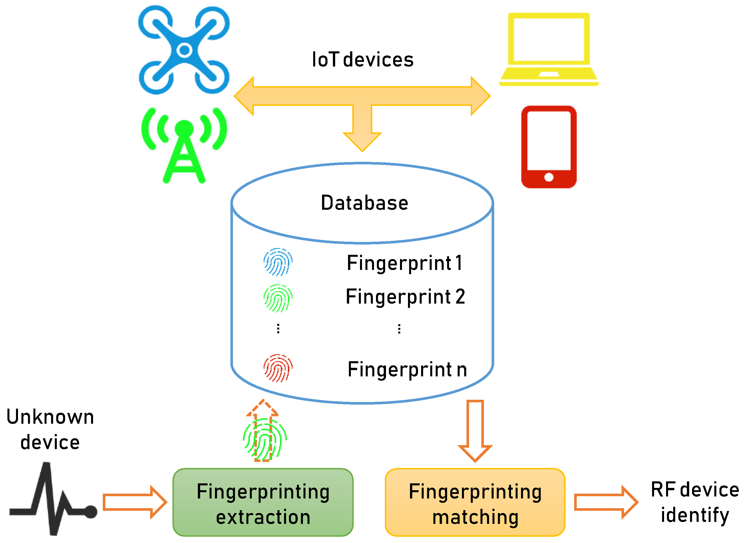
1. Introduction

Today, drones or unmanned aerial vehicles (UAVs) are used to improve our daily lives. Due to the fast development of embedded devices and wireless communications, drones have become cheaper and more powerful. For example, drones contribute to civil areas, such as logistics and agriculture, and play important roles in responding to search and rescue in emergency disasters [1,2]. Drones have become an integral part of society’s rapid development [3,4]. However, the widespread use of drones without government regulations may cause risks related to people’s security and privacy. For example, drones are used by some people to eavesdrop on wireless communication data from long distances [5]. Therefore, relevant authorities have considered the safety and privacy issues involved in drones; efficient identification and detection of drone signals need to be adopted [6].

Radiofrequency (RF) fingerprinting-based recognition technology [7,8,9] is a classification technology based on the physical layer measurements. RF fingerprinting plays an important role in the recognition and detection of drones to accurately identify a variety of Internet of Things (IoT) devices [10]. Because the inherent characteristics and specifications of different IoT devices (e.g., radiofrequency) are not completely consistent, RF fingerprinting technology detects and identifies different devices by extracting subtle differences. In addition, the process of RF fingerprinting recognition usually includes two steps: training and classification [11,12,13], which are shown in Figure 1. First, we use the RF data receiver to collect RF data from different IoT devices, such as nonlinear phase changes and frequency offsets. Subsequently, the RF fingerprinting characteristics of each device were extracted and stored in our database [14]. Second, we can identify and classify the signals of unknown devices according to the prepared RF fingerprinting database obtained in the first step. M. Ezuma et al. [15] used the k-nearest neighbor (KNN) classifier to detect and classify RF signals from different UAV controllers. However, there is an upper limit to the recognition accuracy of RF fingerprinting based on the traditional algorithm and we urgently need better technology with higher recognition performance [16].

Deep learning-aided algorithms [17,18,19,20,21] are widely used in the field of wireless communications and other fields [22,23,24] because due to their efficient feature extraction and recognition capabilities [20,25,26,27,28,29,30,31,32]. Convolutional neural networks (CNNs) have improved the classification accuracies of automatic modulation classifications (AMCs) [33]. Y. Wang et al. [34] proposed a new AMC method combined with two CNNs trained on different datasets and achieved higher identification accuracy. In addition, the use of the DL algorithm in RF fingerprint recognition technology has also led to many outstanding results. For example, L. Peng et al. [35] utilized the differential constellation trace figure (DCTF) and CNN algorithm to achieve 99% recognition accuracy on 54 Zigbee devices.

RF fingerprinting technology based on DL has achieved high classification accuracy based on deep real-valued networks. The RF signals sent by wireless devices combine in-phase and quadrature components. Compared with a deep real-valued network, a deep complex-valued network [36] extracts more abstract data from drone RF signals (the RF signals transmitted from drones), which help to achieve higher classification accuracy. Inspired by this, this paper proposes a DC-CNN-based RF recognition technology to detect different drone signals. Unlike most RF technologies that use real-valued CNN models, our proposed algorithm model is based on a deep complex-valued network, which extracts the hidden features of drone signals with high accuracy in comparison with a real-valued CNN. The main contributions of this article are summarized as follows:

• We propose a drone recognition technology based on a DC-CNN model with improved classification performances within two given independent drone signal datasets.
• Our study used recently published drone datasets [37] in which drone RF data (measured under different operating modes) and background activities were captured in a laboratory setting at Qatar University. This dataset used two RF signal receivers to receive the high and low-frequency signal data of the drone and the entire RF spectrum was obtained by performing a discrete Fourier transform (DFT) on these signal data.
• We present nine different models that compare and evaluate classification performances to show the superior performance of the DC-CNN model. We comprehensively evaluated the performance of each algorithm and found that the proposed DC-CNN model is superior to the other algorithm models.

The remainder of the paper is organized as follows: Section 2 is an overview of the related work. Section 3 introduces our proposed drone recognition system design and some basic theories of the deep complex-valued network. Section 4 provides the architectures of two algorithm models and their training steps. The dataset implementations and simulation results of our drone recognition methods are described in Section 5. Finally, the paper is concluded in Section 6.

2. Related Works

In this section, we first introduce some traditional transmitter device recognition methods based on statistical learning. Then, we focus on RF fingerprinting identification methods based on automatic feature extraction.

2.1. Traditional Transmitter Device Recognition Methods

The traditional transmitter device recognition methods are all based on detecting the unique properties of different transmitters. As we all know, the transmitter sends an instantaneous signal when it starts or stops receiving the RF signal data. During this short period of time (usually a few microseconds), the capacitive load is charged or discharged. In [38], the authors proposed a transmitter classification method based on instantaneous signals; they used a multifractal segmentation method with the same transient concept. Segmentation technology extracts important features from instantaneous signals and generates compact multi-element models. It was shown by the computer simulation that the use of temporal features extracted by the random neural network classifier achieves a classification accuracy of about 90%.

Furthermore, it is important that although the authors use neural networks for final classification, they determine the characteristics of instantaneous signals based on experience, so we consider it to be a traditional method of RF fingerprinting identification. In [39], the authors proposed another transmitter classification method based on instantaneous signals. The KNN discrimination method was used for device identification. This method used instantaneous signals for spectrum feature selection. The author identified a total of eight RF signal transmitters, achieving 97% accuracy at a 30 dB signal-to-noise ratio (SNR) and 66% accuracy at a 0 dB SNR. The above-mentioned are traditional transmitter identification methods, which mainly classify transmitters based on the RF signal characteristics of the transmitter. However, because these characteristics depend on the protocol adopted by the device, any change in the protocol will change the characteristic results, which could make it difficult for traditional methods to identify devices between different types of transmission protocols. As shown in Figure 2, traditional transmitter device recognition methods consist of three steps: signal pre-processing and conversion, feature extraction, and identification. Signal conversion involves converting complex baseband signals from one domain into other domains, and then the pre-designed features are extracted from the converted signals. Finally, based on the extracted features, the machine learning (ML)-based classifier identifies various specific emitters.

2.2. Automatic Feature Extraction-Based RF Fingerprinting Methods

In recent years, researchers have studied the combination of automatic feature extraction with RF fingerprinting techniques. All traditional methods used for RF fingerprinting lack flexibility. These methods require human involvement to determine the features to be extracted (such as instantaneous signals) and design specific algorithms for those features. Automatic feature extraction techniques (such as neural networks) can explore the abstract features of RF data and make classification accuracy higher. In [40], in order to identify the cognitive communication networks, the authors used a CNN model from the DL algorithm to recognize and identify the signals of seven ZigBee devices. The recognition accuracy of this can reach 92.29% in high SNR conditions. However, this algorithm performed poorly in low SNR conditions. In [41], the authors proposed an autoencoder-based indoor location method within the DL algorithm. This algorithm used an autoencoder to achieve high-precision positioning within the RF data collected from the smartphones. As the training dataset increased, the positioning accuracy became more accurate.

As shown in Figure 3, DL-based device recognition methods consist of two steps: signal pre-processing/conversion and identification. After signal pre-processing and conversion, deep neural network models can automatically extract features from the input signal. Finally, the DL-based classifier identifies various specific emitters.

3. System Design and Complex-Valued Network Theory

3.1. System Design

The design of our proposed drone recognition system used in this paper is shown in Figure 4. The signal targets we studied included three different types of running drone signals (drone activities) and noise signals in the space without drones (background activities). According to the drone dataset description that used the RF receiver to collect the drone or background activities signal at multiple times, we first pre-processed those RF data from the prepared drone dataset and made the signal sample sizes of all drone signal classes consistent. Importantly, DC-CNN and various algorithm models were used to train and test these drone signal samples, respectively. Finally, we evaluated the classification performances of all algorithm models in order to verify the superiority of our proposed DC-CNN algorithm.

We used the passive frequency scanning method to obtain the drone operating frequency and carrier frequency restoration between the transmitter and receiver. Since these three drone operating frequencies are Wi-Fi signals near the 2.4 GHz frequency band, we used the passive frequency scanning method to obtain the specific operating frequency of each drone before we collected the signal data. Then, we used the receiver to capture the modulated signal with the drone’s operating frequency as the center frequency. We used two USRP-2943 (NI-USRP) RF receivers to obtain raw drone RF samples. Since the maximum instantaneous bandwidth of each RF receiver was 40 MHz, two receivers were required to operate at the same time to capture the drone Wi-Fi spectrum whose effective bandwidth was at least 80 Mhz. The first receiver captured the lower half of the frequency band and the second receiver recorded the upper half. Finally, the receiver demodulated the modulated signal to obtain the initial baseband data. We assumed that such baseband RF data were better and obtained a near-perfect carrier frequency restoration.

3.2. Deep Complex-Valued Network

Since most of the electromagnetic wave signals are in complex-value forms, compared to real-value networks, the deep complex-valued network is able to extract abstract information from the in-phase and quadrature parts of the signal. Therefore, it is particularly important to introduce the theory of a deep complex-valued network in RF research; two complex-valued network concepts used in this article are explained.

3.2.1. Complex-Valued Convolution Operation

The core part of a CNN is its convolution operation, which can extract various abstract features from the network input and reduce network parameters. Similarly, a complex-valued convolution operation is the core part of a DC-CNN and it can be implemented by superposing multiple real-valued convolution operations. The process of a complex-valued convolution operation between a complex-valued feature map $\mathit{M}$ and the complex-valued convolution kernel $\mathit{K}$ is shown in Figure 5. As we can see from the figure, the green part ${\mathit{M}}_R$ represents the real part of $\mathit{M}$, the blue part of ${\mathit{K}}_R$ represents the real part of $\mathit{K}$, the red part ${\mathit{M}}_I$ represents the imaginary part of $\mathit{M}$, and the yellow part ${\mathit{K}}_I$ represents the imaginary part of $\mathit{K}$. After the complex-valued convolution operation is completed, the output of the feature map is divided into real and imaginary parts. Finally, we can obtain the complete complex-valued convolution calculation function as

$$\begin{array}{c}\hfill \mathit{M}\ast \mathit{K}=({\mathit{M}}_R{\mathit{K}}_R-{\mathit{M}}_I{\mathit{K}}_I)+i({\mathit{M}}_R{\mathit{K}}_I+{\mathit{M}}_I{\mathit{K}}_R).\end{array}$$

(1)

3.2.2. Complex-Valued Weight Initialization

The complex-valued weight initialization can effectively reduce the disappearance of the gradients and accelerate the convergence of the complex-valued neural network. A complex-valued weight $\mathit{W}$ can be expressed in polar or matrix coordinates:

$$\begin{array}{c}\hfill \mathit{W}=\left|\mathit{W}\right|e^{i\theta }=\mathrm{Re}\left[\mathit{W}\right]+i\mathrm{Im}[\mathit{W}],\end{array}$$

(2)

among them, $\mathbf{\theta }$ and $\left|\mathit{W}\right|$ are the phase and modulus values of $\mathit{W}$, respectively. The variance of $\mathit{W}$ is defined as:

$$\begin{array}{c}\hfill Var\left(\mathit{W}\right)=\mathrm{E}[\mathit{W}{\mathit{W}}^{*}]-{(\mathrm{E}[\mathit{W}])}^2=\mathrm{E}[{\left|\mathit{W}\right|}^2]-{\left(\mathrm{E}\left[\mathit{W}\right]\right)}^2,\end{array}$$

(3)

when $\mathit{W}$ is center-symmetrically distributed about 0, the variance of $\mathit{W}$ is simplified as $\mathrm{E}\left[{\left|\mathit{W}\right|}^2\right]$. On the other hand, the variance of $\left|\mathit{W}\right|$ can be expressed as:

$$\begin{array}{c}\hfill Var\left(\left|\mathit{W}\right|\right)=\mathrm{E}\left[{\left|\mathit{W}\right|}^2\right]-{\left(\mathrm{E}\left[\left|\mathit{W}\right|\right]\right)}^2.\end{array}$$

(4)

In summary, we can define the variance of $\mathit{W}$ as:

$$\begin{array}{c}\hfill Var\left(\mathit{W}\right)=Var\left(\left|\mathit{W}\right|\right)+{\left(\mathrm{E}\left[\left|\mathit{W}\right|\right]\right)}^2,\end{array}$$

(5)

if the modulus value of $\left|\mathit{W}\right|$ obeys the Rayleigh distribution, the mathematical expectation and variance of $\left|\mathit{W}\right|$ are calculated as follows:

$$\begin{array}{c}\hfill \left\{\begin{array}{c}\mathrm{E}\left[\left|\mathit{W}\right|\right]=\sigma \sqrt{\frac{\pi }{2}}\hfill \\ Var\left(\left|\mathit{W}\right|\right)=\frac{4-\pi }{2}{\sigma }^2,\hfill \end{array}\right.\end{array}$$

(6)

where $\sigma$ is the parameter of the Rayleigh distribution. Bringing Function (6) into Function (5), we can obtain the variance of $\mathit{W}$ as:

$$\begin{array}{c}\hfill Var\left(\mathit{W}\right)=\frac{4-\pi }{2}{\sigma }^2+\frac{\pi }{2}{\sigma }^2=2{\sigma }^2,\end{array}$$

(7)

through this formula, we can implement the modulus value initialization of the complex-valued weight $\mathit{W}$. In addition, the phase initialization of $\mathit{W}$ can be done by choosing uniformly distributed values, obeying $[-\pi ,\pi ]$.

3.2.3. Complex-Valued Batch Normalization

Batch normalization (BN) involves accelerating the training process and avoiding overfitting. Given that the b-th real-valued input in a batch is ${\{{\mathit{I}}_b^R\}}_{b=1}^B$, where B is the number of training samples in a batch, and the i-th element of ${\mathit{I}}_b^R$ is defined as $I_{b,i}^R$, the real-valued BN ($rBN$) can be formulated as

$$\begin{array}{c}\hfill f_{rBN}(I_{b,i}^R)=\gamma \frac{I_{b,i}^R-{\mu }_B}{\sqrt{{\sigma }_B^2+ϵ}}+\beta ,\end{array}$$

(8)

where ${\mu }_B$ is the mean of $I_{b, i}^R,b\in [1,B]$ in a batch; ${\sigma }_B^2$ is the variance; $ϵ$ prevents ${\sigma }_B^2$ from being zero; $\gamma$ and $\beta$ are two learnable parameters. In the complex-valued BN ($cBN$), the i-th element of the complex-valued input in a batch is defined as $I_{b,i}^C=\mathfrak{R}(I_{b,i}^C)+j·\mathfrak{I}(I_{b,i}^C)$. Then, the real and imaginary parts of $I_{b,i}^C$ are split to form a matrix ${\mathit{I}}_{b,i}^C={\left[\begin{array}{c}\mathfrak{R}(I_{b,i}^C)\\ \mathfrak{I}(I_{b,i}^C)\end{array}\right]}_{2\times 1}$. Similar to $rBN$, $cBN$ can be expressed as

$$\begin{array}{c}\hfill f_{cBN}({\mathit{I}}_{b,i}^c)=\mathit{\gamma }{({\mathit{\sigma }}_B^2+\mathit{ϵ})}^{-\frac{1}{2}}[{\mathit{I}}_{b,i}^c-{\mathit{\mu }}_B]+\mathit{\beta },\end{array}$$

(9)

$${\mathit{\sigma }}_B^2=\left[\begin{array}{cc}Va{r}_{\mathfrak{R}}& Co{v}_{\mathfrak{R}\mathfrak{I}}\\ Co{v}_{\mathfrak{I}\mathfrak{R}}& Va{r}_{\mathfrak{I}}\end{array}\right], {\mathit{\mu }}_B=\left[\begin{array}{c}\frac{1}{B}\sum _{b=1}^B\mathfrak{R}(I_{b,i}^C)\\ \frac{1}{B}\sum _{b=1}^B\mathfrak{I}(I_{b,i}^C)\end{array}\right],$$

(10)

$$\mathit{\gamma }=\left[\begin{array}{cc}{\gamma }_{\mathfrak{R}\mathfrak{R}}& {\gamma }_{\mathfrak{R}\mathfrak{I}}\\ {\gamma }_{\mathfrak{I}\mathfrak{R}}& {\gamma }_{\mathfrak{I}\mathfrak{I}}\end{array}\right], \mathit{\beta }=\left[\begin{array}{c}{\beta }_{\mathfrak{R}}\\ {\beta }_{\mathfrak{I}}\end{array}\right],\mathit{ϵ}=\left[\begin{array}{cc}ϵ& 0\\ 0& ϵ\end{array}\right],$$

(11)

where ${(·)}^{-1/2}$ is an inverse operation with taking square root; $Co{v}_{\mathfrak{R}\mathfrak{I}}$ (or $Co{v}_{\mathfrak{I}\mathfrak{R}}$) is the covariance between ${\{\mathfrak{R}(I_{b,i}^C)\}}_{b=1}^B$ and ${\{\mathfrak{I}(I_{b,i}^C)\}}_{b=1}^B$; $Va{r}_{\mathfrak{R}}$ and $Va{r}_{\mathfrak{I}}$ are the variances of ${\{\mathfrak{R}(I_{b,i}^C)\}}_{b=1}^B$ and ${\{\mathfrak{I}(I_{b,i}^C)\}}_{b=1}^B$, respectively.

3.2.4. Complex-Valued Activation Function

The complex-valued activation function is similar to a real-valued activation function. For example, the rectified linear unit ($ReLU$) is a general activation function for DL, and the real-valued ReLU ($rReLU$) can be written as

$$\begin{array}{c}\hfill f_{rReLU}({\mathit{I}}^R)=\max ({\mathit{I}}^R,0),\end{array}$$

(12)

while the complex-valued ReLU ($cReLU$) can be expressed as

$$\begin{array}{c}\hfill f_{cReLU}({\mathit{I}}^C)=\max (\mathfrak{R}({\mathit{I}}^C),0)+j·\max (\mathfrak{I}({\mathit{I}}^C),0).\end{array}$$

(13)

4. Algorithm Model and Implementation

In this section, we focus on two DL algorithm models. We first introduce an existing classification algorithm model: convolutional, long short-term memory, fully connected deep neural network (CLDNN), which incorporates three classic DL algorithm models. Next, we will elaborate on the DC-CNN algorithm proposed in this paper for drone detection, which is extended from a deep real-valued CNN (DR-CNN). Finally, the architecture of another DL algorithm and specific training steps are described.

4.1. Architecture of CLDNN

CLDNN combines the advantages of three DL algorithm models: CNN, long short-term memory (LSTM), and deep neural network (DNN). The architecture of the CLDNN model is depicted in Figure 6. In addition to the input and output layers, the CLDNN model includes the convolutional part, the LSTM part, and the fully connected (FC) part. The sample size of the drone dataset used in this paper is $2\times 2048$, which is also the size of the input layer.

This model has two convolutional layers—one LSTM layer and three FC layers. The size of the convolutional kernel in the first convolution layer is $2\times 4$, and in the second convolutional layer is $1\times 8$. In order to better extract the features, the convolutional kernel numbers in the two convolutional layers are 128 and 64, respectively, and the only LSTM layer has 256 neurons. In addition, the activation functions of the convolutional and LSTM layers are $ReLU$, and the dropout layer is behind each of them in order to reduce overfitting and accelerate the network convergence. Moreover, the neuron numbers in the three FC layers are 256, 128, and M (the type of drones to be distinguished). By connecting the FC layer with the $Softmax$ activation function, we can output the predicted probability of the target drone and realize the drone recognition.

4.2. Architecture of DC-CNN

DC-CNN is used to extract hiding features from drone signals because it has a much more powerful and effective feature representation and classification capability than DR-CNN in signal identification. Unlike the CLDNN model, the proposed DC-CNN algorithm model in this paper is based on the fusion of a traditional CNN and deep complex-valued network. The architecture of the DC-CNN model used in drone detection is depicted in Figure 7. In addition to the input and output layers, our proposed DC-CNN model includes a complex-valued convolutional part and a complex-valued FC part, which use the theory of a complex-valued convolution operation and complex-valued weight initialization, as described in Section 4. The sample size of the drone dataset used in this paper is $2\times 2048$, which is also the input size in our proposed model. Moreover, the specific parameter settings are based on our training experience and were adjusted after multiple experiments to achieve the best recognition ability.

Our proposed DC-CNN model has two complex-valued convolutional layers and three complex-valued FC layers. The size of the complex-valued convolutional kernel in the first complex-valued convolution layer is 16, and in the second complex-valued convolutional layer is 8. In order to better extract features, the complex-valued convolutional kernel numbers in the two complex-valued convolutional layers are 128 and 64, respectively, and all complex-valued convolution layers use one-dimensional complex-valued convolution ($cConv1D$). Additionally, the activation functions of complex-valued convolutional layers are complex-valued $ReLU$ ($cReLU$) and the dropout layer is behind each of them in order to reduce overfitting and accelerate network convergence. Moreover, the neuron numbers in the three complex-valued FC layers are 256, 128, and M (the type of drones to be distinguished). By connecting the complex-valued FC layer with one $Softmax$ activation function, we can output the predicted probability of the target drone and realize drone detection.

4.3. Architecture of Other DL Models

As mentioned above, in reference [40], the author used a real-valued convolutional neural network to identify RF data. In this paper [37], the author used three-layered fully connected neural network structures to identify drone signals. We also used these two DL models for comparative experiments to show our superiority. The rest of the DL models used in this paper contain DR-CNN (Conv2D) and DR-CNN (Conv1D) in [40], a fully connected neural network (FCN) in [37], and LSTM models, whose architectures are shown in

Table 1. Structures and sizes of other DL models.

Algorithm	Conv. Layer	LSTM Layer	FC Layer	Model Size
DR-CNN (Conv2D)	{128, 64}	/	{256, 128, 64, M}	33,891,912
DR-CNN (Conv1D) [40]	{128, 64}	/	{256, 128, 64, M}	33,859,656
FCN [37]	/	/	{512, 256, 128, M}	2,267,400
LSTM	/	{256, 128}	{256, 128, 64, M}	2,665,160

.

4.4. Training Process of DL-Based Drone Recognition Method

The DL-based drone RF fingerprinting recognition method is modeled as a multi-class classification problem and cross-entropy (CE) is generally applied as its loss function. Suppose that the training samples and labels are ${\{{\mathit{S}}_n,{\mathit{L}}_n\}}_{n=1}^N$, the CE loss function can be expressed as:

$$\begin{array}{c}\hfill \begin{array}{cc}\hfill \mathcal{L}(f_{DL},\mathit{W};{\{{\mathit{S}}_n,{\mathit{L}}_n\}}_{n=1}^N)=& -\frac{1}{N}\sum _{n=1}^N{\mathit{L}}_n\log [f_{DL}(\mathit{W};{\mathit{S}}_n)],\hfill \end{array}\end{array}$$

(14)

this function represents the CE loss function, which can indicate the classification performance; $f_{DL}$ represents the mapping between the input and output of the DL model and $\mathit{W}$ is its weight. Considering that we have thousands of samples for each training, it is impossible to put them into the network simultaneously. Our model training batch size is 64, which means that the loss value for each calculation is calculated from 64 drone samples.

Additionally, $Adam$ is used as the optimizer for DL-based methods, which can be written as:

$$\begin{array}{cc}\hfill & m_{t+1}={\beta }_1{m}_t+(1-{\beta }_1)\frac{\partial \mathcal{L}}{\partial w},w\in \mathit{W},\hfill \end{array}$$

(15)

$$\begin{array}{cc}\hfill & v_{t+1}={\beta }_2{v}_t+(1-{\beta }_2){(\frac{\partial \mathcal{L}}{\partial w})}^2,\hfill \end{array}$$

(16)

$$\begin{array}{cc}\hfill & {\widehat{m}}_{t+1}=\frac{m_{t+1}}{1-{\beta }_1^t},{\widehat{v}}_{t+1}=\frac{v_{t+1}}{1-{\beta }_2^t},\hfill \end{array}$$

(17)

$$\begin{array}{cc}\hfill & w_{t+1}=w_t-{\eta }_t\frac{{\widehat{m}}_{t+1}}{\sqrt{{\widehat{v}}_{t+1}}+ϵ},\hfill \end{array}$$

(18)

where $m_t$ and $v_t$ are the biased first and second-moment estimates; ${\widehat{m}}_t$ and ${\widehat{v}}_t$ are the bias-corrected first and second-moment estimates; $\frac{\partial \mathcal{L}}{\partial w}$ is the gradient; ${\beta }_1$ and ${\beta }_2$ are the decaying factors; ${\eta }_t$ is the learning rate; $ϵ$ is the minimum.

Finally, the entire proposed intelligent drone recognition algorithm steps are presented. Algorithm 1 lists the pseudo-code of the DL-based drone RF fingerprinting recognition method.

Algorithm 1 The proposed DL-based drone recognition method.

Require:  IQ samples with the size of $2\times 2048$; Ensure:  The best algorithm model for the drone detection method;   1: initial $g_0=0$ and $d_0=0$;   2: Select IQ samples in drone datasets and mix them randomly;   3: Initialize the complex-valued neural network weight parameter $\mathit{W}$;   4: Divide all drone datasets into training sets and testing sets within 7:3;   5: Send the IQ samples to different DL models for training. The structure and parameters of the CLDNN algorithm model are shown in Figure 6 and those of DC-CNN are shown in Figure 7;   6: Test and verify data multiple times in order to obtain the average recognition accuracy and each sample’s running GPU time;   7: Evaluate the various indicators of each algorithm and achieve the best algorithm for the drone recognition method;   8: return The best algorithm model.

4.5. Comparison Method: TD Feature with ML Recognizers

Here, we adopt a TD feature and ML-based drone recognition as the comparison method, which is given as follows.

4.5.1. Pre-Processing & Conversion

Convert the complex baseband signal into other forms. For instance, the complex baseband signal is defined as $S(k),0\le k\le K-1$, and $S(k)=I(k)+j·Q(k),0\le k\le K-1$, where $I(k)$ and $Q(k)$ are the in-phase and quadrature components, respectively, and K is the number of sampling points. In the time domain, the baseband signal can be converted into instantaneous amplitude $\alpha (k)=\sqrt{I^2(k)+Q^2(k)}$, instantaneous phase $\varphi (k)=\arctan [\frac{Q(k)}{I(k)}]$, and instantaneous frequency $f(k)=\frac{1}{2\pi }\frac{d\varphi (k)}{dk}$. In addition, the conversion can also be performed by wavelet transform, Hilbert–Huang transform, or differential constellation trace figures.

4.5.2. Feature Extraction

Here, we mostly introduce the time domain (TD) features [42]. In detail, the first step of feature extraction is to evenly divide the converted signal component into multiple slices. Assuming that the converted signal component is $\mathit{S}=[s_0,s_1,\cdots ,s_{K-1}]$, the length of each slice is $L_s$, and the number of slices is $K_s=K/L_s$, the i-th component slice can be written as

$$\begin{array}{c}\hfill {\mathit{S}}^i=[s_{(i-1)L_s},s_{(i-1)L_s+1},\cdots ,s_{i{L}_s-1}],1\le i\le K_s.\end{array}$$

(19)

Features are extracted from each slice ${\mathit{S}}^i,1\le i\le K_s$, and the total signal component $\mathit{S}$. The typical features are the standard deviation $\sigma$, variance ${\sigma }^2$, skewness $\gamma$, and kurtosis $\kappa$. The four features extracted from the i-th slice can consist of a feature vector ${\mathit{F}}_i={[{\sigma }_i,{\sigma }_i^2,{\gamma }_i,{\kappa }_i]}_{1\times 4}$. Next, these feature vectors ${\{{\mathit{F}}_i\}}_{i=1}^{K_s}$ and ${\mathit{F}}_{total}$, respectively, are extracted from each slice and total signal component, and are integrated into the final feature vector $\mathit{F}={[{\mathit{F}}_1\cdots {\mathit{F}}_2\cdots {\mathit{F}}_{K_s}\cdots {\mathit{F}}_{total}]}_{1\times 4(K_s+1)}$ for traditional transmitter device recognition.

Except for the above TD features, energy entropy, the first moments, and the second order moment are useful temporal features, while spectral flatness, spectral brightness, and spectral roll-off are effective spectral features.

4.5.3. Recognition-Based on ML

With the development of ML, some ML recognizers, such as SVM, random forest (RF), decision tree (DT), and so on, are applied to identify various specific emitters based on the above extracted feature.

5. Results and Discussion

In this section, the performance of our proposed DC-CNN algorithm model is demonstrated and analyzed using two different drone datasets. We compared a total of nine different machine learning or DL models, all of which were trained within independent training and testing datasets. We comprehensively evaluated all algorithms in the classification accuracy, sample running time, model size, and so on. The details are shown below.

5.1. Dataset Description and Experimental Setup

Similar to most DL-based RF fingerprinting research studies, we used two RF receivers to receive high-frequency and low-frequency signals when multiple drones were running. The portable computer was used to perform DFT to the RF data collected from two RF receivers and connect them to form the entire drone RF spectrum. We used two independent RF fingerprint-based drone datasets for training and testing. In

Table 2. Details of the two used drone datasets in our experiment.

Category	Classes	Samples
Dataset 1
background	background activities	1100
drone	drone {1, 2, 3} activities	3300
Dataset 2
drone 1	modes {connect, hover, fly, record}	4400
drone 2	modes {connect, hover, fly, record}	4400

, we provide all details of the drone datasets used in our simulation experiment. Dataset 1 contained four classes of drone data: background activities (noise signals in the space without drones), drone 1 activities, drone 2 activities, and drone 3 activities. Those three drone activities were in flight modes without any instructions or operations. This dataset was used to verify whether our proposed DC-CNN could identify different drones accurately. Moreover, dataset 2 contained RF data collected from two kinds of drones in four different operating modes, including connecting modes (connecting to the controller), automatic hovering modes (without other instructions), straight flight modes (flying without video recording), and recording modes (flying with video recording). Two different drones were tested and collected data in four different operating modes, totaling eight classes of drone data. This dataset was used to verify whether our proposed DC-CNN could perform better in identifying the different operating modes of one drone. The size of each class of RF samples is $2\times 2048$ and its number is 1100, which means that there are 4400 samples in dataset 1 and 8800 samples in dataset 2.

Moreover, extensive experiments were performed in order to evaluate the classification performances of our proposed DC-CNN model. We used one RF signal collector and one computer, which included two operating systems: Window10 and Ubuntu 16.04.1-Linux. Further, the computer contained 8 Intel Xeon E3 (x 86_64) central processing units (CPUs) and 4 NVIDIA GTX1080Ti graphic processing units (GPUs), which could efficiently handle various matrix multiplication and convolution operations. On the one hand, the Windows system mainly uses MATLABR2019a software to preprocess RF drone data. On the other hand, the Linux system mainly uses $spyder5.3.1$ software for training and testing DL models. In addition, we used the $Keras2.2.2$ software library based on $Python3.7.1$ language to complete the construction of DL models.

5.2. Accuracy of DL and Traditional Algorithm Methods within Two Datasets

Accuracies of the comparisons and traditional algorithms are shown in Figure 8; all 9 algorithm models were used to distinguish between dataset 1, which contained 4400 samples, and dataset 2, which contained 8800 samples. As the number of classification samples increased, the recognition accuracy decreased, as expected. The downward trend of each algorithm was basically the same. We first compared the accuracy of our proposed DC-CNN algorithm with traditional signal processing algorithms, such as random forest with time domain features (TD-RF), decision tree with time domain features (TD-DT), and support vector machine with time domain features (TD-SVM). Compared with the DL models, the accuracies of the traditional signal processing algorithms dropped faster.

In order to further compare the performance of our proposed algorithm, we selected popular DL algorithms for training, such as CLDNN, DR-CNN (Conv2D), and LSTM. The recognition accuracy of LSTM is not ideal, meaning that it is not suitable for recognizing drone signals. The accuracies of the three DL algorithms were very close, which indicated that they all could effectively identify the signal. The CLDNN model had a (more than) 30% higher recognition accuracy than DR-CNN (Conv2D). The DR-CNN (Conv1D) model had a (more than) 30% higher recognition accuracy than the FCN model in dataset 2. In addition, we compared FCN and DR-CNN (Conv1D); DC-CNN was more capable of identifying different drone RF signals. The accuracies of most algorithms decreased in a nonlinear manner.

As shown in

Table 3. Classification accuracies of different drone recognition methods.

Accuracy (%)	Dataset 1	Dataset 2
DC-CNN (proposed)	99.50	74.10
CLDNN	97.65	70.36
DR-CNN (Conv2D)	92.93	59.28
DR-CNN (Conv1D) [40]	91.46	66.44
FCN [37]	85.05	42.12
LSTM	55.63	23.94
TD-RF	86.74	46.78
TD-DT	53.93	22.69
TD-SVM	23.48	12.05

, we compared the classification accuracies of nine algorithms in total. The recognition accuracy of the DC-CNN model in four classes was 99% and dropped to 74% in eight classes. When training on dataset 1, the recognition accuracies of the first four algorithms in Table 1 were all higher than 90%. In addition, compared to classic DL models (CNN, FCN, LSTM), DC-CNN and CLDNN models were more capable of identifying different drone RF signals. The DC-CNN model proposed in this paper achieved the best recognition accuracies in two datasets, which were 99.5% and 74.1%, respectively.

Additionally, it can be clearly seen from Table 3 that DR-CNN (Conv2D) performed better than DR-CNN (Conv1D) in dataset 1, but it had lower accuracy than DR-CNN (Conv1D) in dataset 2. The size of the input drone RF datum was $2\times 2048$, which is two-dimensional; considering the excellent performance of the CNN in image recognition, we expanded the two-dimensional data into three-dimensional data in the DR-CNN (Conv2D) input layer in order to extract features better. In this case, DR-CNN (Conv2D) was accomplished at processing three-dimensional data, and the recognition accuracy should have been better than that of DR-CNN (Conv1D), as reflected in dataset 1. However, the recognition performance of DR-CNN (Conv2D) in dataset 2 had a 7% lower recognition accuracy than DR-CNN (Conv1D). We believe that DR-CNN (Conv2D) had an overfitting phenomenon in training, which led to the low test results.

5.3. Learning Curves of Different DL Models in Different Datasets

This section will illustrate the training processes of models that obtained the top three recognition accuracies and analyze the loss convergence speeds between different models. Figure 9 shows the convergence curve in dataset 1. These three algorithms converged quickly, all approaching 0. Figure 10 shows the convergence curve in dataset 2. Due to the increased difficulty in identification, the convergence speed slowed down. In particular, compared with CLDNN and DR-CNN, the DC-CNN model designed in this paper was always the first to achieve convergence, and its loss value was closer to 0. In addition, although the convergence speed of CLDNN was slower than that of DR-CNN, its final loss value was lower than that of CNN, and the recognition performance was better.

5.4. Algorithm System Comparison

Figure 11 depicts the running GPU time required for each algorithm to identify a single drone sample and the total parameters contained in that algorithm model. It can be seen from the figure that the parameters included in one model were not directly related to the GPU time. We can clearly see that the total model parameters of the DC-CNN model were roughly the same as DR-CNN (Conv1D) and FCN models, but the GPU time of the DC-CNN model was much less than those in the two datasets. In addition, the CLDNN model’s GPT time is similar to that of the DR-CNN model, but the total model parameters are four times that of the DR-CNN model. Further, we can conclude that the recognition accuracy of CLDNN is higher than most other algorithms (obtained at the cost of too many model parameters and running times). In summary, we conclude that even if the complex-valued network has the same parameters as the real-valued network, the complex-valued network has a lower processing time and faster recognition speed.

5.5. Confusion Matrix of the DC-CNN Model in Different Datasets

Subsequently, we show the confusion matrices of our proposed DC-CNN model within different datasets in Figure 12 and Figure 13. These percentage matrices can apparently reflect some details that cannot be seen above. Figure 12 represents dataset 1 (four classes) and Figure 12 represents dataset 2 (eight classes). By observing the diagonals of all the confusion matrices, we can see the recognition performance of our algorithm model for each class. First, we find that the DC-CNN model can accurately identify each type of drone signal in dataset 1. Even in the worst case, the classification accuracy of background activity signals can achieve 98.5%. Moreover, for dataset 2, the name of each class is composed of M and two numbers—the first number indicating the drone model and the second number indicating the running mode of the drone. For example, the meaning of $\mathbf{M}\mathit{12}$ is the signal received by the first drone in mode 2. Therefore, we can easily understand that the DC-CNN model is difficult to identify the signal of the second drone in mode 3 ($\mathbf{M}\mathit{23}$), whose identification accuracy is only 4.88%.

We can see that from four to eight classes, the accuracy of our proposed DC-CNN model reduces by about 25%. In dataset 1, the signals from the different categories of drones are distinguished, and the physical properties of their signal transmitters are very different, which is easy to recognize. However, we mainly focus on distinguishing the signals in different operating modes of the same drone in dataset 2, which is much more difficult. There are mainly two difficulties that lead to errors. First, the identification errors between different operating mode signals are from the same drone (e.g., 53.28% of the D2 record is recognized as the D2 connect). Second, identification errors of the same operating mode signal are from different types of drones (e.g., 65.92% of the D2 fly is recognized as the D1 fly). This is also the main reason for the decline in the accuracy of the DC-CNN model within dataset 2.

5.6. Additive Evaluation of DC-CNN Model in Different Datasets

Finally, we evaluate the performance of the DC-CNN algorithm model in two datasets from other aspects. The additive performance evaluation indicators that we used in this paper are $Precision$, $Recall$, and $F1score$. The definitions of precision and recall are as follows:

$$\begin{array}{c}\hfill Precision=\frac{TP}{TP+FP}\end{array}$$

(20)

$$\begin{array}{c}\hfill Recall=\frac{TP}{TP+FN}\end{array}$$

(21)

Among them, TP, FP, and FN indicate true positive, false positive, and false negative, respectively. The value of the $F1score$ is determined by the values of $Precision$ and $Recall$, whose definition is:

$$\begin{array}{c}\hfill F1score=2\left(\frac{Precision\times Recall}{Precision+Recall}\right)\end{array}$$

(22)

As shown in Figure 14 and Figure 15, blue is the $Precision$ value, green is the $Recall$ value, and the red curve represents the $F1score$ for each class. The values of these three evaluation indicators in Figure 14 are all above 98%, showing that the DC-CNN model performs excellent in identifying drone dataset 1. In addition, we can clearly see from Figure 15 that the three indicators of DC-CNN in drone dataset 2 perform very well in most classes. However, the recognition performance of the $\mathbf{M}\mathbf{23}$ class seems to be worse; the $Recall$ and $F1score$ values do not even reach 10%. Moreover, we observe that the $Precision$ value of $\mathbf{M}\mathbf{13}$ and the $Recall$ value of $\mathbf{M}\mathbf{24}$ are only about 50%, which will be the focus of our next research study.

6. Conclusions

In this paper, we proposed a new drone recognition method based on DC-CNN. Unlike conventional DR-CNN methods, our proposed DC-CNN method can extract more hidden features from drone RF signals that have in-phase and quadrature parts. We used nine different drone recognition algorithm models that were trained separately on two independent datasets and evaluated their performances regarding their classifications, GPU times, and parameters. The experimental results show that the classification accuracy of the DC-CNN model to identify dataset 1 was 99.5%, and that of dataset 2 was 74.1%. Simulation results prove that our proposed algorithm performs well compared to other existing DL-based drone recognition algorithms. In future work, we will consider further optimizing network parameters and running times.

References

- Liu, M.; Yang, J.; Gui, G. DSF-NOMA: UAV-assisted emergency communication technology in a heterogeneous internet of things. IEEE Internet Things J. 2019, 6, 5508–5519. [Google Scholar] [CrossRef]
- Liu, M.; Tang, F.; Kato, N.; Adachi, F. 6G: Opening new horizons for integration of comfort, security and intelligence. IEEE Wirel. Commun. Mag. 2020, 27, 126–132. [Google Scholar]
- Mohanti, S.; Soltani, N.; Sankhe, K.; Jaisinghani, D.; Felice, M.D.; Chowdhury, K. AirID: Injecting a custom RF fingerprint for enhanced UAV identification using deep learning. In Proceedings of the IEEE Global Communications Conference (GLOBECOM), Taipei, Taiwan, 7–11 December 2020; pp. 1–9. [Google Scholar]
- Jagannath, A.; Jithin, J.; Kumar, P. A comprehensive survey on radio frequency (rf) fingerprinting: Traditional approaches, deep learning, and open challenges. arXiv 2022, arXiv:2201.00680. [Google Scholar] [CrossRef]
- Shoufan, A.; Al-Angari, H.M.; Sheikh, M.F.A.; Damiani, E. Drone pilot identification by classifying radio-control signals. IEEE Trans. Inf. Forensics Secur. 2018, 13, 2439–2447. [Google Scholar] [CrossRef]
- Al-Emadi, S.; Al-Ali, A.; Mohammad, A.; Al-Ali, A. Audio based drone detection and identification using deep learning. In Proceedings of the International Wireless Communications and Mobile Computing Conference (IWCMC), Tangier, Morocco, 24–28 June 2019; pp. 459–464. [Google Scholar]
- Gong, J.; Xu, X.; Lei, Y. Unsupervised specific emitter identification method using radio-frequency fingerprint embedded infoGAN. IEEE Trans. Inf. Forensics Secur. 2020, 15, 2898–2913. [Google Scholar] [CrossRef]
- Su, H.-R.; Chen, K.-Y.; Wong, W.J.; Lai, S.-H. A deep learning approach towards pore extraction for high-resolution fingerprint recognition. In Proceedings of the IEEE International Conference on Acoustics, Speech, & Signal Processing (ICASSP), New Orleans, LA, USA, 5–9 March 2017; pp. 2057–2061. [Google Scholar]
- Roy, D.; Mukherjee, T.; Chatterjee, M.; Blasch, E.; Pasiliao, E. RFAL: Adversarial learning for RF transmitter identification and classification. IEEE Trans. Cogn. Commun. Netw. 2020, 6, 783–801. [Google Scholar] [CrossRef]
- Tian, X.; Wu, X.; Li, H.; Wang, X. RF fingerprints prediction for cellular network positioning: A subspace identification approach. IEEE Trans. Mob. Comput. 2020, 19, 450–465. [Google Scholar] [CrossRef]
- Wang, Y.; Gui, G.; Gacanin, H.; Ohtsuki, T.; Dobre, O.A.; Poor, H.V. An efficient specific emitter identification method based on complex-valued neural networks and network compression. IEEE J. Sel. Areas Commun. 2021, 39, 2305–2317. [Google Scholar] [CrossRef]
- Satyanarayana, K.; El-Hajjar, M.; Mourad, A.A.M.; Hanzo, L. Deep learning aided fingerprint-based beam alignment for mmWave vehicular communication. IEEE Trans. Veh. Technol. 2019, 68, 10858–10871. [Google Scholar] [CrossRef]
- Peng, Y.; Liu, P.; Wang, Y.; Gui, G.; Adebisi, B.; Gacanin, H. Radio frequency fingerprint identification based on slice integration cooperation and heat constellation trace figure. IEEE Wirel. Commun. Lett. 2022, 11, 543–547. [Google Scholar] [CrossRef]
- Lin, Y.; Zhu, X.; Zheng, Z.; Dou, Z.; Zhou, R. The individual identification method of wireless device based on dimensionality reduction and machine learning. J. Supercomput. 2019, 75, 3010–3027. [Google Scholar] [CrossRef]
- Ezuma, M.; Erden, F.; Anjinappa, C.K.; Ozdemir, O.; Guvenc, I. Detection and classification of UAVs using RF fingerprints in the presence of Wi-Fi and bluetooth interference. IEEE Open J. Commun. Soc. 2020, 1, 60–76. [Google Scholar] [CrossRef]
- Yang, K.; Kang, J.; Jang, J.; Lee, H.N. Multimodal sparse representation-based classification scheme for RF fingerprinting. IEEE Commun. Lett. 2019, 23, 867–870. [Google Scholar] [CrossRef]
- Li, C. Dynamic offloading for multiuser muti-CAP MEC networks: A deep reinforcement learning approach. IEEE Trans. Veh. Technol. 2021, 70, 2922–2927. [Google Scholar] [CrossRef]
- Zheng, Q.; Yang, M.; Yang, J.; Zhang, Q.; Zhang, X. Improvement of Generalization Ability of Deep CNN via Implicit Regularization in Two-Stage Training Process. IEEE Access 2018, 6, 15844–15869. [Google Scholar] [CrossRef]
- Zhao, M.; Jha, A.; Liu, Q.; Millis, B.A.; Jansen, A.M.; Lu, L.; Landman, B.A.; Tyska, M.J.; Huo, Y. Faster Mean-shift: GPU-accelerated clustering for cosine embedding-based cell segmentation and tracking. Med. Image Anal. 2021, 71, 102048. [Google Scholar] [CrossRef]
- Zhao, M.; Liu, Q.; Jha, A.; Deng, R. VoxelEmbed: 3D instance segmentation and tracking with voxel embedding based deep learning. In Proceedings of the International Workshop on Machine Learning in Medical Imaging, Strasbourg, France, 27 September 2021; Springer: Cham, Switzerland, 2021. [Google Scholar]
- Jin, B.; Cruz, L.; Gonçalves, N. Pseudo RGB-D Face Recognition. IEEE Sens. J. 2022, 22, 21780–21794. [Google Scholar] [CrossRef]
- Wang, Z. An adaptive deep learning-based UAV receiver design for coded MIMO with correlated noise. Phys. Commun. 2021, 45, 101292. [Google Scholar] [CrossRef]
- Huang, H.; Peng, Y.; Yang, J.; Xia, W.; Gui, G. Fast beamforming design via deep learning. IEEE Trans. Veh. Technol. 2020, 69, 1065–1069. [Google Scholar] [CrossRef]
- He, K.; He, L.; Fan, L.; Deng, Y.; Karagiannidis, G.K.; Nallanathan, A. Learning based signal detection for MIMO systems with unknown noise statistics. IEEE Trans. Commun. 2021, 69, 3025–3038. [Google Scholar] [CrossRef]
- Lai, S.; Zhao, R.; Tang, S.; Xia, J.; Zhou, F.; Fan, L. Intelligent secure mobile edge computing for beyond 5G wireless networks. Phys. Commun. 2021, 45, 101283. [Google Scholar] [CrossRef]
- Gu, H.; Wang, Y.; Hong, S.; Gui, G. Blind channel identification aided generalized automatic modulation recognition based on deep learning. IEEE Access 2019, 7, 110722–110729. [Google Scholar] [CrossRef]
- Sun, J.; Shi, W.; Han, Z.; Yangi, J. Behavioral modeling and linearization of wideband RF power amplifiers using BiLSTM networks for 5G wireless systems. IEEE Trans. Veh. Technol. 2019, 68, 10348–10356. [Google Scholar] [CrossRef]
- Gacanin, H. Autonomous wireless systems with artificial intelligence: A knowledge management perspective. IEEE Veh. Technol. Mag. 2019, 14, 51–59. [Google Scholar] [CrossRef]
- Guo, Y.; Zhao, Z.; He, K.; Lai, S.; Xia, J.; Fan, L. Efficient and flexible management for industrial internet of things: A federated learning approach. Comput. Netw. 2021, 192, 1–9. [Google Scholar] [CrossRef]
- Shi, Z.; Gao, W.; Zhang, S.; Liu, J.; Kato, N. AI-enhanced cooperative spectrum sensing for non-orthogonal multiple access. IEEE Wirel. Commun. Mag. 2020, 27, 173–179. [Google Scholar] [CrossRef]
- Tang, F.; Kawamoto, Y.; Kato, N.; Liu, J. Future intelligent and secure vehicular network towards 6G: Machine-learning approaches. Proc. IEEE 2020, 108, 292–307. [Google Scholar] [CrossRef]
- Wang, Y.; Gui, J.; Yin, Y.; Wang, J.; Sun, J. Automatic modulation classification for MIMO systems via deep learning and zero-forcing equalization. IEEE Trans. Veh. Technol. 2020, 69, 5688–5692. [Google Scholar] [CrossRef]
- Wang, Y.; Gui, G.; Gacanin, H.; Adebisi, B.; Sari, H.; Adachi, F. Federated learning for automatic modulation classification under class imbalance and varying noise condition. IEEE Trans. Cogn. Commun. Netw. 2022, 8, 86–96. [Google Scholar] [CrossRef]
- Wang, Y.; Yang, J.; Liu, M.; Gui, G. LightAMC: Lightweight automatic modulation classification using deep learning and compressive sensing. IEEE Trans. Veh. Technol. 2020, 69, 3491–3495. [Google Scholar] [CrossRef]
- Peng, L.; Zhang, J.; Liu, M.; Hu, A. Deep learning based RF fingerprint identification using differential constellation trace figure. IEEE Trans. Veh. Technol. 2020, 69, 1091–1095. [Google Scholar] [CrossRef]
- Zhang, Z.; Wang, H.; Xu, F.; Jin, Y.Q. Complex-valued convolutional neural network and its application in polarimetric SAR image classification. IEEE Trans. Geosci. Remote. Sens. 2017, 55, 7177–7188. [Google Scholar] [CrossRef]
- Al-Sa’d, M.; Al-Ali, A.; Mohamed, A.; Khattab, T.; Erbad, A. RF-based drone detection and identification using deep learning approaches: An initiative towards a large open source drone database. Future Gener. Comput. Syst. 2019, 100, 86–97. [Google Scholar] [CrossRef]
- Shaw, D.; Kinsner, W. Multifractal modelling of radio transmitter transients for classification. In Proceedings of the IEEE WESCANEX 97 Communications, Power and Computing. Conference Proceedings, Winnipeg, MB, Canada, 22–23 May 1997; pp. 306–312. [Google Scholar]
- Kennedy, I.O.; Scanlon, P.; Mullany, F.J.; Buddhikot, M.M.; Nolan, K.E.; Rondeau, T.W. Radio transmitter fingerprinting: A steady state frequency domain approach. In Proceedings of the IEEE 68th Vehicular Technology Conference (VTC2008-Fall), Calgary, AB, Canada, 21–24 September 2008; pp. 1–5. [Google Scholar]
- Merchant, K.; Revay, S.; Stantchev, G.; Nousain, B. Deep learning for RF device fingerprinting in cognitive communication networks. IEEE J. Sel. Top. Signal Process. 2018, 12, 160–167. [Google Scholar] [CrossRef]
- Khatab, Z.E.; Hajihoseini, A.; Ghorashi, S.A. A fingerprint method for indoor localization using autoencoder based deep extreme learning machine. IEEE Sens. Lett. 2018, 2, 2057–2061. [Google Scholar] [CrossRef]
- Li, Y.; Chen, X.; Lin, Y.; Srivastava, G.; Liu, S. Wireless transmitter identification based on device imperfections. IEEE Access 2020, 8, 59305–59314. [Google Scholar] [CrossRef]