Article

Processing and Interpretation of UAV Magnetic Data: A Workflow Based on Improved Variational Mode Decomposition and Levenberg–Marquardt Algorithm

1
Aerospace Information Research Institute, Chinese Academy of Sciences, Beijing 100094, China
2
Key Laboratory of Electromagnetic Radiation and Sensing Technology, Chinese Academy of Sciences, Beijing 100190, China
3
School of Electronic, Electrical and Communication Engineering, University of Chinese Academy of Sciences, Beijing 100049, China
*
Author to whom correspondence should be addressed.
Drones 2022, 6(1), 11; https://doi.org/10.3390/drones6010011
Submission received: 26 November 2021 / Revised: 28 December 2021 / Accepted: 30 December 2021 / Published: 3 January 2022
(This article belongs to the Special Issue Unmanned Aerial System in Geomatics)

Abstract

:
Unmanned aerial vehicles (UAVs) have become a research hotspot in the field of magnetic exploration because of their unique advantages, e.g., low cost, high safety, and easy to operate. However, the lack of effective data processing and interpretation method limits their further deployment. In view of this situation, a complete workflow of UAV magnetic data processing and interpretation is proposed in this paper, which can be divided into two steps: (1) the improved variational mode decomposition (VMD) is applied to the original data to improve its signal-to-noise ratio as much as possible, and the decomposition modes number K is determined adaptively according to the mode characteristics; (2) the parameters of target position and magnetic moment are obtained by Euler deconvolution first, and then used as the prior information of the Levenberg–Marquardt (LM) algorithm to further improve its accuracy. Experiments are carried out to verify the effectiveness of the proposed method. Results show that the proposed method can significantly improve the quality of the original data; by combining the Euler deconvolution and LM algorithm, the horizontal positioning error can be reduced from 15.31 cm to 4.05 cm, and the depth estimation error can be reduced from 16.2 cm to 5.4 cm. Moreover, the proposed method can be used not only for the detection and location of near-surface targets, but also for the follow-up work, such as the clearance of targets (e.g., the unexploded ordnance).

1. Introduction

Unmanned aerial vehicles (UAVs) have been applied in many fields during the past decade, e.g., remote sensing, geological prospecting, and unexploded ordnance (UXO) detection [1,2,3]. Among these applications, the use of UAV for magnetic survey is a booming branch [4]. Compared with the traditional terrestrial magnetic survey, a UAV magnetic survey can cover a wider range with a higher efficiency. Besides, it is also easy to operate, low-cost, and has good safety compared with the manned aircraft magnetic survey. Moreover, a UAV magnetic survey can be conducted in areas that are difficult to access or would pose a potential hazard to operators, which means that some gaps in traditional magnetic surveys can now be studied [5,6].
Considerable progress has been made in the integration of UAV magnetic systems in the past decade, however, the low quality of UAV magnetic data and the lack of effective data interpretation methods have become the biggest obstacles to its further development. Several attempts have been made to improve the quality of UAV magnetic data, e.g., the magnetic gradiometer is towed about 2 m below the UAV in [7] to mitigate the interference generated by the platform; a similar method is also adopted in [8,9,10,11]. However, this design introduced the directional and positional error, meanwhile increasing the risk of impact to the magnetometers. Filtering methods [12,13,14] are considered to improve the quality of UAV magnetic data, however, there are three main shortcomings: (1) filter parameters need to be determined according to a priori knowledge; (2) the frequency characteristic of the target signal will change with the conditions, such as the flight speed of the platform, which means that the parameters of the filter should also be changed, and (3) once the frequencies of the target signal and noise overlap, the filtering method will be difficult to apply. Liu et al. [15] proposed an adaptive elimination method of geomagnetic background noise, but it should be noted that this method requires an additional magnetometer, which means a shorter flight time for UAV magnetic systems.
Recently, a method based on the empirical mode decomposition (EMD) and its improved form has been applied to UAV magnetic data processing [16]. Although the effectiveness of this method has been proven by experimental results, the processing workflow is somewhat complex, and meanwhile, the physical meaning of the obtained intrinsic mode function (IMF) is not obvious. Inspired by this successful case, variational mode decomposition (VMD) is introduced in this paper for the processing of UAV magnetic data. To the best of our knowledge, this is the first time that VMD has been applied to this field. VMD is a completely non-recursive decomposition method proposed by Dragomiretskiy et al. [17], and has been widely used in gear fault diagnosis, feature extraction, and seismic time-frequency analysis [18,19,20]. However, the performance of VMD is affected by the decomposition modes number K, under-decomposition or over-decomposition will occur if K is not appropriate. In [21], K is set to be consistent with that of EMD, which is obviously not convenient. Appropriate K can be obtained by using the optimization algorithm [22], but it is time-consuming and inefficient. Previous studies [23,24] have shown that the mode characteristics can be used to optimize K, and this method is also used in this paper.
Once K is determined, the original data can be processed, and the magnetic map of the survey area can be obtained. The anomalies caused by ferromagnetic targets will be reflected in the magnetic map, and the parameter estimation of these targets is the main task of data interpretation [25]. Euler deconvolution [26,27,28] is often used to estimate the position and magnetic moment of the target. Davis et al. [29] proposed a terrestrial magnetic survey workflow for the detection of UXO by using sliding window-based Euler deconvolution, however, the changing size of the sliding window makes the process complex and cumbersome. Zhou and Zhang [30] proposed a method for the location of multiple magnetic targets by combining gradient tensor inversion and K-means clustering. Simulation results show that the positioning error of this method is about 0.05 m, which is acceptable for most applications. In addition, methods based on Euler deconvolution, such as tilt-Euler deconvolution [31] and joint-gradient Euler deconvolution [32], have also been proposed to better interpret magnetic data.
The optimization method is a good choice considering the overdetermined problem to be solved here. Ding et al. [33] proposed a new method for estimating locations and moments of multiple dipole-like magnetic sources using differential evolution (DE); the results of synthetic and field tests showed that the location of magnetic source can be estimated well. A local optimization method, the Levenberg–Marquardt (LM) algorithm, is introduced in this paper to obtain a more accurate estimation of the target parameters. LM algorithm, also known as the Damped Least Squares (DLS) algorithm, is very suitable for solving the nonlinear problem with the advantage of fast convergence [34,35,36]. The result of Euler deconvolution is used as the initial value of the LM algorithm. By minimizing the misfit between the predicted and observed magnetic anomalies, the target location accuracy can be significantly improved. It should be noted that the proposed method is not superior to other methods such as DE but provides a simple and fast methodology in target parameters estimation.
All in all, the main contributions of this manuscript are as follows:
  • A complete workflow based on the improved VMD, and the joint Euler deconvolution-LM algorithm is proposed for the processing and interpretation of UAV magnetic data.
  • The VMD method is applied for the processing of UAV magnetic data, and the decomposition modes number K is adaptively determined according to the mode characteristics.
  • The positioning accuracy of near-surface targets is significantly improved by combining Euler deconvolution and the LM algorithm without increasing too much complexity, which is very helpful for the follow-up work.
The rest of this paper is organized as follows: Section 2 presents the related theories of VMD, Euler deconvolution, and LM algorithms. The proposed workflow for the processing and interpretation of UAV magnetic data is described in detail in Section 3. Experiments are carried out, and the results are analyzed in Section 4. Section 5 is the discussion and final remarks of the proposed workflow.

2. Theoretical Background

The proposed method can be divided into two steps, namely, magnetic data processing based on the improved VMD method and magnetic data interpretation based on the combined Euler deconvolution-LM algorithm. The theory and implementation of the relevant methods are briefly introduced in this part.

2.1. Magnetic Data Processing

2.1.1. VMD Algorithm

As declared in [17], VMD decomposes the original signal x ( t ) into K band-limited IMFs, which have the sparsity properties, the narrow-band IMF u k ( t ) , k = 1 , 2 , , K is defined as an amplitude-modulated-frequency-modulated (AM-FM) signal, as given by:
u k ( t ) = A k ( t ) cos ( ϕ k ( t ) ) ,
where A k ( t ) and ϕ k ( t ) are the instantaneous amplitude and phase, respectively. The instantaneous frequency ω k ( t ) is defined as the derivative of ϕ k ( t )
ω k ( t ) = d ϕ k ( t ) / d t = ϕ k ( t ) .
The Hilbert transform is applied to each mode, then the mode’s spectrum is shifted to baseband according to Fourier transform. After that, the Gaussian smoothness is used to estimate the bandwidth of each mode. The constrained variational problem of VMD is given by:
min { u k } , { ω k } { k = 1 K t [ ( δ ( t ) + j π t ) * u k ( t ) ] e j ω k t 2 2 } s . t . k = 1 K u k = x ( t ) ,
where { u k } and { ω k } are the K mode components and center frequencies, respectively. δ ( t ) is the Dirac distribution, * refers to convolution, and 2 2 is the square of the Euclidean norm. (3) can be transformed into unconstrained problem by utilizing the quadratic penalty factor α and Lagrange multiplier λ ( t ) , the augmented Lagrangian form of (3) can be expressed as:
L ( { u k } , { ω k } , λ ) = α k = 1 K t [ ( δ ( t ) + j π t ) * u k ( t ) ] e j ω k t 2 2 + x ( t ) k = 1 K u k 2 2 + λ ( t ) , x ( t ) k = 1 K u k ,
where a , b represents the inner product of a and b . To solve this unconstrained variational problem, the alternate direction method of multipliers is applied, and the values of u k , ω k , and λ are updated in frequency respectively. u k can be updated using the equivalent minimization problem, defined as follows:
u k n + 1 ( t ) = argmin u k X { α t [ ( δ ( t ) + j π t ) * u k ( t ) ] e j ω k t 2 2 + x ( t ) i u i ( t ) + λ ( t ) 2 2 2 } ,
where X is the functional space of signal and modes, the n and n + 1 are omitted for the fixed ω k and u i k .
The formula for updating u k , ω k , and λ are given by:
u ^ k n + 1 ( ω ) = [ x ^ ( ω ) i k u ^ i ( ω ) + λ ^ ( ω ) 2 ] 1 1 + 2 α ( ω ω k ) 2
ω k n + 1 = 0 ω | u ^ k ( ω ) | 2 d ω 0 | u ^ k ( ω ) | 2 d ω
λ ^ n + 1 ( ω ) = λ ^ n ( ω ) + τ [ x ^ ( ω ) k u ^ k n + 1 ( ω ) ] ,
where u ^ k ( ω ) , x ^ ( ω ) , and λ ^ ( ω ) are the Fourier transform of u k ( t ) , x ( t ) , and λ ( t ) . τ is the parameter of noise tolerance. The above calculation is continuously implemented until the following iteration termination condition is met:
k u ^ k n + 1 u ^ k n 2 2 / u ^ k n 2 2 < ε ,
where ε is the tolerance parameter of the convergence criterion. The default values of ε and τ of the standard VMD are utilized in this study.
A key parameter affecting the performance of VMD is the selection of the decomposition modes number K. Previous studies are generally based on experience or optimization algorithms to determine K, but all these methods present drawbacks. Ref. [23] proposed an adaptive VMD method for signal processing based on mode characteristics, several indicators, e.g., permutation entropy (PE), extreme value in frequency domain, kurtosis, dominant frequency spacing between neighboring modes, and energy loss coefficient are used to determine K. Li et al. [37] put forward a frequency-aided method to solve the problem of choosing parameters for VMD and judged whether the decomposition was excessive by comparing the difference of IMF center frequencies. Inspired by these studies, an improved VMD method based on mode characteristics is utilized in the following subsection to determine K.

2.1.2. The Improved VMD Algorithm

As mentioned earlier, inappropriate K can lead to under-decomposition or over-decomposition, which both affect the performance of VMD. Here, we propose an improved VMD method which is completely data-driven and based on the mode characteristics to determine K. The method mainly consists of six steps, explained as follows:
  • The starting point is to determine the following parameters: the minimum mode number K m i n , the maximum mode number K m a x , the threshold μ , and the penalty parameter α ;
  • Let K = K m i n , perform VMD on the input signal x ( t ) , a set of IMFs can be obtained and recorded as { I M F i , K , i [ 1 , K ] } , the corresponding center frequencies are recorded as { f i , K , i [ 1 , K ] } ;
  • Let K n = K + 1 , we can also obtain a set of IMFs and the corresponding center frequencies, namely, { I M F p , K n , p [ 1 , K n ] } , and { f p , K n , p [ 1 , K n ] } ;
  • Compare { f i , K } and { f p , K n } to determine the new center frequency in { f p , K n } , and the IMF corresponding to the new center frequency is obtained as r ( t ) ;
  • Calculate the correlation coefficients { C o e f i } between r ( t ) and { I M F i , K } ;
  • Execute judgement, if “ C o e f i > μ ” is true, it means that the decomposition is excessive, then make the optimal decomposition number K b e s t = K . Otherwise, continue to implement 3–5 until the criterion is met.
In this paper, the threshold μ is set to 0.4 empirically, besides, to judge whether there is under-decomposition or not, we introduce the energy loss coefficient e l which is defined as the energy ratio of the decomposition residual to the original signal [23]:
e l = x ( t ) k u k 2 2 x ( t ) 2 2 ,
where u k is the kth IMF, and k u k is the reconstructed signal. When under-decomposition occurs, there is a large error between the reconstructed signal and the original signal, which means that the e l is also relatively large. Therefore, the under-decomposition can be determined by judging whether the e l is greater than the threshold δ . In this paper, δ is set to 0.1. By using the above method, a suitable K can be obtained, which can be used to process the UAV magnetic data.

2.2. Magnetic Data Interpretation

After completing the processing of the UAV magnetic data, the data interpretation, or inversion, can be carried out. The purpose of data interpretation is to infer the parameters of the target, e.g., the spatial position and magnetic moment, from the observed magnetic anomalies. Euler deconvolution has been adapted as a tool for the quick initial interpretation due to its simplicity. However, Euler deconvolution, like other geophysical inversion methods, can only provide the approximate location of the target, which cannot meet our requirements. Therefore, an optimization method based on the LM algorithm is proposed to further improve the target positioning accuracy. The Euler deconvolution and the LM algorithm are introduced in the following subsections, respectively.

2.2.1. Euler Deconvolution

The theoretical basis of Euler deconvolution is that the magnetic anomaly field generated by the target satisfies the following Euler’s homogeneity equation [26,29]:
T x ( x x 0 ) + T y ( y y 0 ) + T z ( z z 0 ) = N T ,
where T is the observed field at ( x , y , z ) generated by the target at location ( x 0 , y 0 , z 0 ) , N denotes the structural index (SI) which varies with different source types.
Applying (11) to several neighboring data points with a prior value for N, the location of the target can be solved in the least squares sense as follows:
P = ( A T A ) 1 A T b ,
P = [ x 0 y 0 z 0 ] , A = [ T 1 x T 1 y T 1 z T 2 x T 2 y T 2 z T n x T n y T n z ] , b = [ x 1 T 1 x + y 1 T 1 y + z 1 T 1 z + N T 1 x 2 T 2 x + y 2 T 2 y + z 2 T 2 z + N T 2 x n T n x + y n T n y + z n T n z + N T n ] ,
where n is the number of data points.
Usually, a specified size of window is used to select the neighboring data points, and the observed magnetic anomalies of these data points are thought to be caused by an isolated target.

2.2.2. Implementation of the LM Algorithm

Generally, the magnetic anomaly field generated by the near-surface target can be considered as a magnetic dipole [38], which can be calculated by:
B = μ 0 4 π [ 3 ( m · r ) r r 5 m r 3 ] ,
where μ 0 is the permeability in vacuum, m is the dipole moment of the target, r is the displacement vector from the target to the measurement point, and r = | r | . The anomaly field generated by the target is usually much smaller than the geomagnetic field, hence the observed anomaly signal Δ B is the projection of the anomaly field in the direction of the geomagnetic field [39], which can be expressed as:
Δ B = f ( r , m ) = B B e | B e | ,
where B e and | B e | are the geomagnetic field and its magnitude, respectively. The main task of data interpretation is to invert the position and magnetic moment of the target through the magnetic anomaly data ( Δ B i , i = 1 , 2 , , N ) of multiple observation points ( r i , i = 1 , 2 , , N ) . By minimizing the misfit between the observed anomaly field Δ B i and the predicted anomaly field f i based on (15), the objective function can be established and expressed as follows:
x * = min x g ( x ) = i = 1 N ( f i ( x ) Δ B i ) 2 .
where x = ( r x , r y , r z , m x , m y , m z ) is the parameter of the target, N is the number of observation points. In fact, (16) is a least square problem which can be solved by the LM algorithm. The following update is used in the LM method to avoid the problem of rank-defect of Jacobian matrix that may occur in the Gauss–Newton method:
x k + 1 = x k ( J ( x k ) T J ( x k ) + λ k I ) 1 J ( x k ) T r ( x k ) ,
where J ( x k ) is the Jacobian matrix that contains the first derivatives of the residual r ( x k ) , and
r ( x k ) = [ f 1 ( x k ) Δ B 1 f 2 ( x k ) Δ B 2 f N ( x k ) Δ B N ] ,
I is the unit matrix, and λ k represents the search direction. If λ k = 0 , LM algorithm becomes the Gauss–Newton method, and when λ k is large, the LM algorithm becomes gradient descent with a small step size. Therefore, the search direction of the LM method combines the Gauss–Newton method and the steepest descent method. More details about LM algorithm can be found in [34,35,36]. It is worth emphasizing that due to the use of Taylor expansion for approximation, an implicit premise is that an initial value must be provided. Here, the solution of Euler deconvolution is used as the initial value of the LM method.

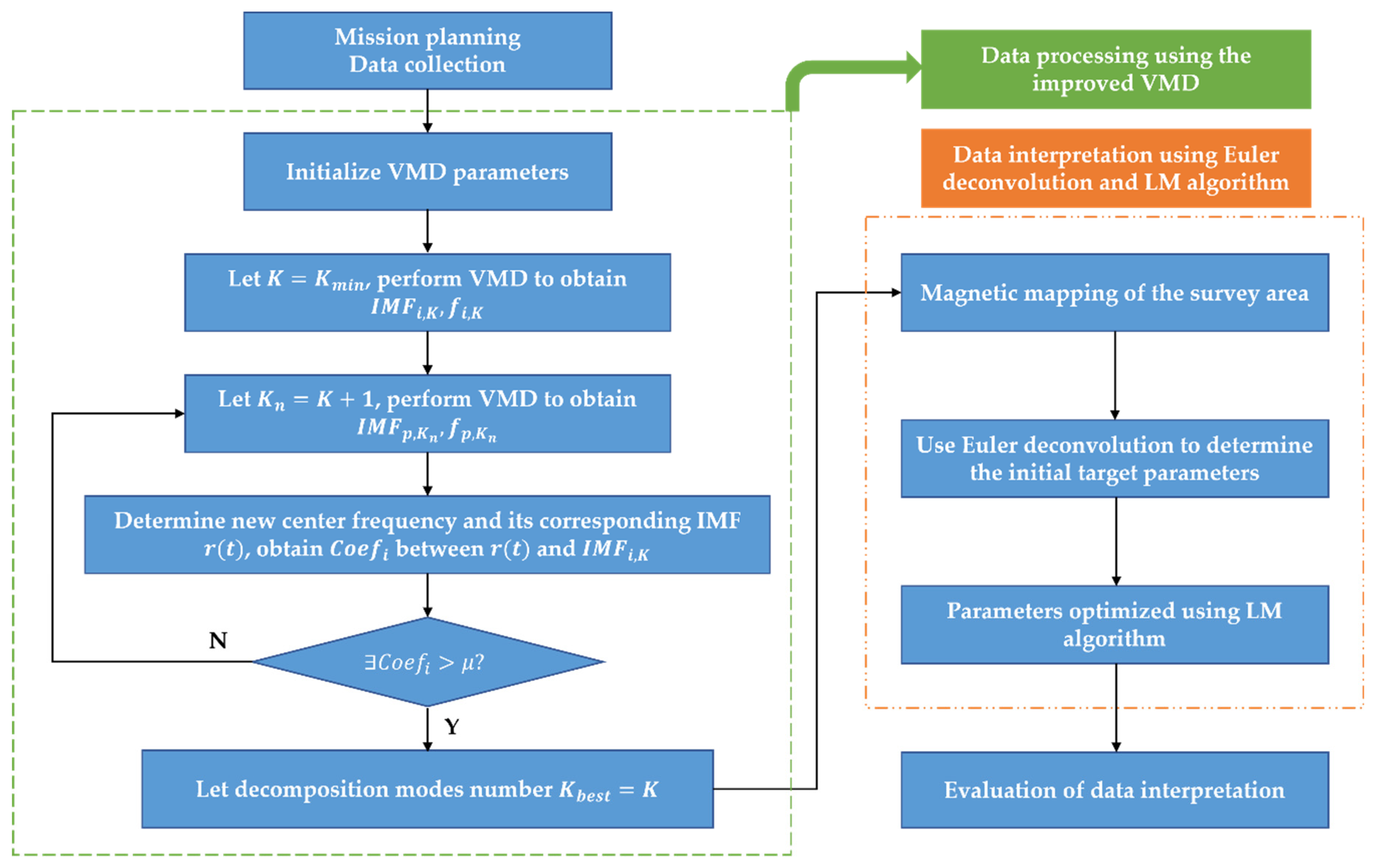
3. The Proposed Workflow Using Improved VMD and Joint Euler-LM Algorithm

This paper proposes a complete workflow for the processing and interpretation of UAV magnetic data, which can be mainly divided into two parts: (1) data processing based on the improved VMD method, where the optimal decomposition modes number K is determined adaptively by mode characteristics, and (2) data interpretation conducted by Euler deconvolution and LM algorithm to obtain a more realistic position and magnetic moment parameters of the target. The proposed workflow is depicted in Figure 1. The steps of the workflow can be summarized as follows:
Step 1:Mission planning is the first step for UAV magnetic survey, many factors, e.g., the survey task, target size, topography of the survey area and weather conditions should be carefully considered to determine the parameters of line spacing, flight altitude and speed. Then, the data collection can be carried out.
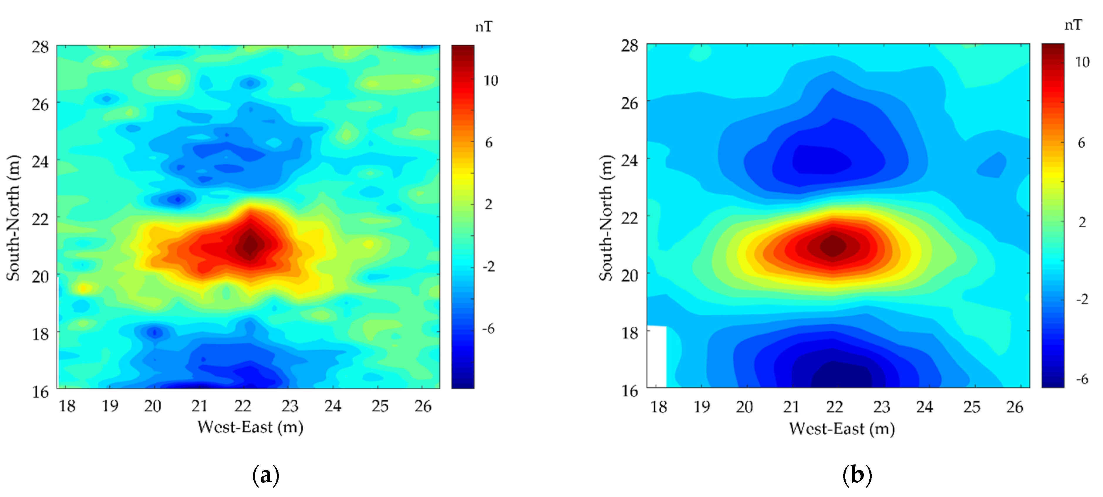
Step 2:Data of each flight profile are processed according to the improved VMD method described in Section 2.1.2, then the magnetic map of the survey area is obtained by interpolation.
Step 3:Euler deconvolution is used to obtain the preliminary estimation of target position and magnetic moment, and these results are then used as the initial value of the LM algorithm to obtain more accurate target parameters.
Step 4:The result of data interpretation is finally evaluated according to the real situation, and the follow-up work (e.g., the clearance of the target) can be carried out.

4. Field Experiments and Analysis

In this section, field experiments are carried out to prove the feasibility of the proposed method. Firstly, the UAV magnetic survey system is briefly introduced. Then, the collection of UAV magnetic data is described in detail. After that, the data processing results are compared with several common schemes. Finally, the parameter estimation of the target is obtained based on the joint Euler deconvolution-LM method, and the effectiveness of the proposed method is verified according to the real situation.

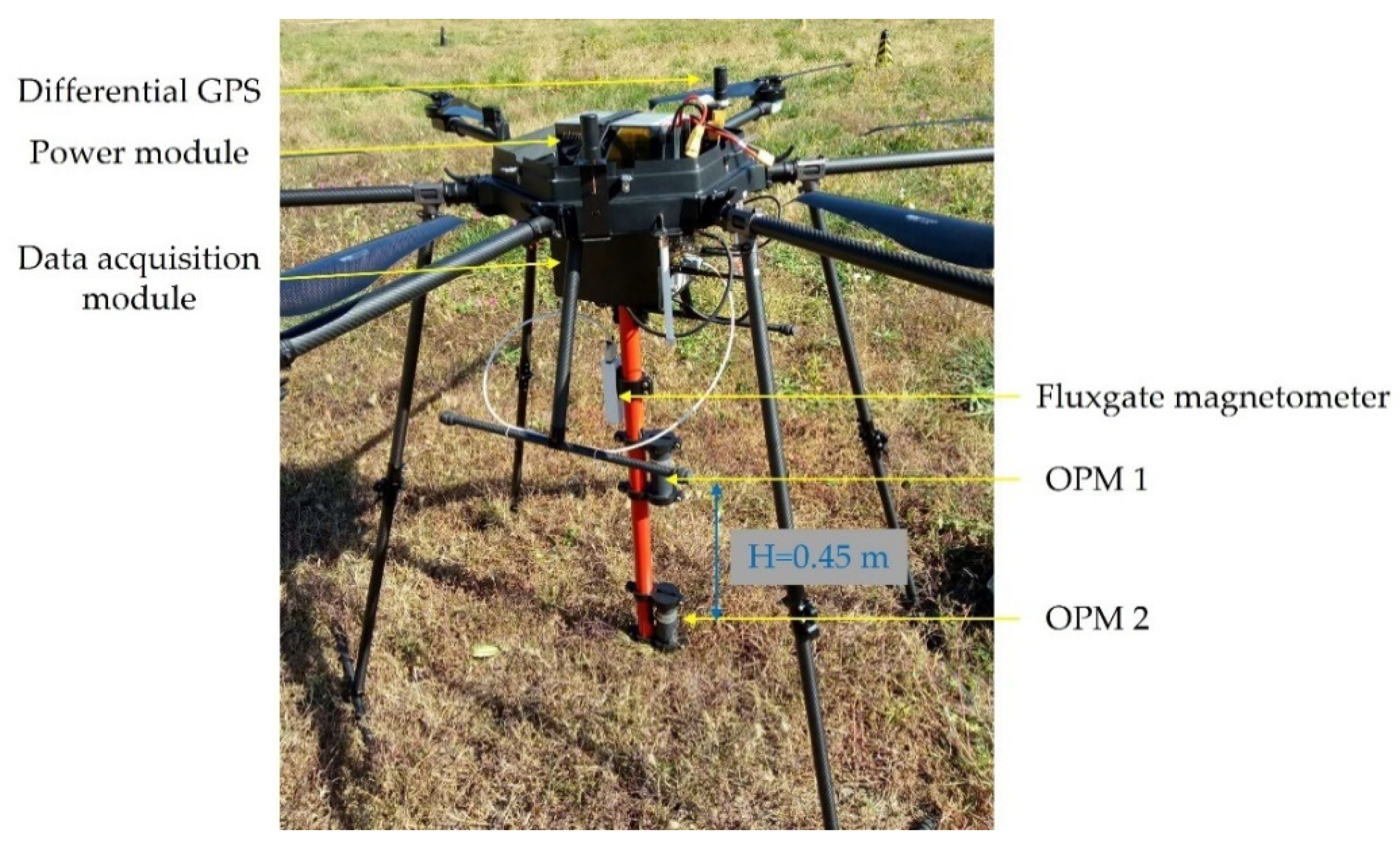
4.1. UAV Magnetic Survey System

A six-rotor-based UAV magnetic survey system has been deployed for the purpose of near-surface targets detection, as shown in Figure 2. The detailed parameters of the system can be found in [16], which is provided in the Supplementary Materials. This system consists of two cesium optically pumped magnetometers (OPMs) and a fluxgate magnetometer to record the total magnetic intensity (TMI) data and the vector magnetic intensity (VMI) data, a differential GPS to provide the location of the UAV, a data acquisition module, and a power module. The two OPMs are rigidly mounted below the center of the UAV by a boom, with a vertical distance of 0.45 m. The TMI and VMI data are synchronized by the pulse per second signal with a sampling frequency of 160 Hz.

4.2. The Collection of UAV Magnetic Data

As we mentioned in Section 3, the line spacing, flight altitude and speed are determined according to a variety of factors, e.g., the task purpose, target size, topography of the survey area, and weather conditions. Considering that the survey area for our experiment is quite flat, a constant flight altitude is adopted. It should be noted that in areas with complex terrain, it is necessary to use a radar (or laser) altimeter with the function of terrain following. The data used in Section 4.3 are obtained from a maneuvering experiment with a flight altitude of 20 m above ground level (AGL), and a speed of about 4 m/s. For the near-surface targets detection application, the flight altitude and line spacing are usually determined through field experiments. For the field experiment proposed in Section 4.4, the flight altitude is set to 2 m AGL, with a line spacing of 0.75 m and a speed of about 2 m/s. The sampling interval along the profile is about 1 cm. The data acquisition module collects differential GPS and magnetic data at the same time and stores them in the SD card.

4.3. UAV Magnetic Data Processing

Data containing 6000 sampling points can be obtained after the UAV maneuvers back and forth along a preset path; the flight altitude of the UAV is about 20 m. The original data and its time-frequency spectrogram after DC component removed are shown in Figure 3.
Three features can be observed from Figure 3: (1) the signal-to-noise ratio (SNR) of the original data is low due to the influence of many kinds of noise; (2) there are two kinds of noise which are obviously different from the target signal in frequency, including the power frequency interference (energy concentrated in 50 Hz) and the interference generated by the platform, the energy of which is distributed in the frequency band of 30-40 Hz; and (3) there are some periodic signals in the frequency band of 0.5–3 Hz, which should be related to the maneuver of the platform. To make a better comparison, EMD is first applied to the original data, 10 IMFs and their corresponding spectrum are obtained, as shown in Figure 4.
As can be seen from Figure 4, the boundary effects and mode mixing are inevitable in EMD. In addition, how to reconstruct signal is a key problem because the physical meaning of the obtained IMFs is not obvious; this uncertainty is caused by the weak mathematical theory of the EMD method itself. Therefore, the VMD method is expected to achieve better results by constructing and solving variational problems.
According to Figure 3b and Figure 4, the decomposition modes number K of VMD is set from 4 to 7, and the penalty factor α is set to 2000. The center frequencies of IMFs obtained and the energy loss coefficient e l with different K are shown in Table 1. The center frequency of IMF1 is close to DC, so it is no longer listed in Table 1.
It can be found that, when K < 6, the energy loss coefficient is greater than 0.1, which means that the signal has not been completely decomposed. When K increases from 6 to 7, the center frequency of the new IMF is very close to that of the previous IMFs, and the change of the energy loss coefficient is very small, which means that over-decomposition may occur at this time. To further confirm the best K, the correlation coefficients between the new IMF (decomposition number = K) and the previous IMFs (decomposition number = K − 1) are calculated according to the method proposed in Section 2.1.2, and the results are shown in Table 2.
When K = 7, IMF4 is a new frequency component, and the correlation coefficient between it and the corresponding IMF4 when K = 6 is 0.6327, greater than the preset threshold, which means that the over-decomposition occurs. Therefore, the optimal decomposition modes number is set to 6. The corresponding decomposition result is shown in Figure 5.
The following conclusions can be drawn from Figure 5:
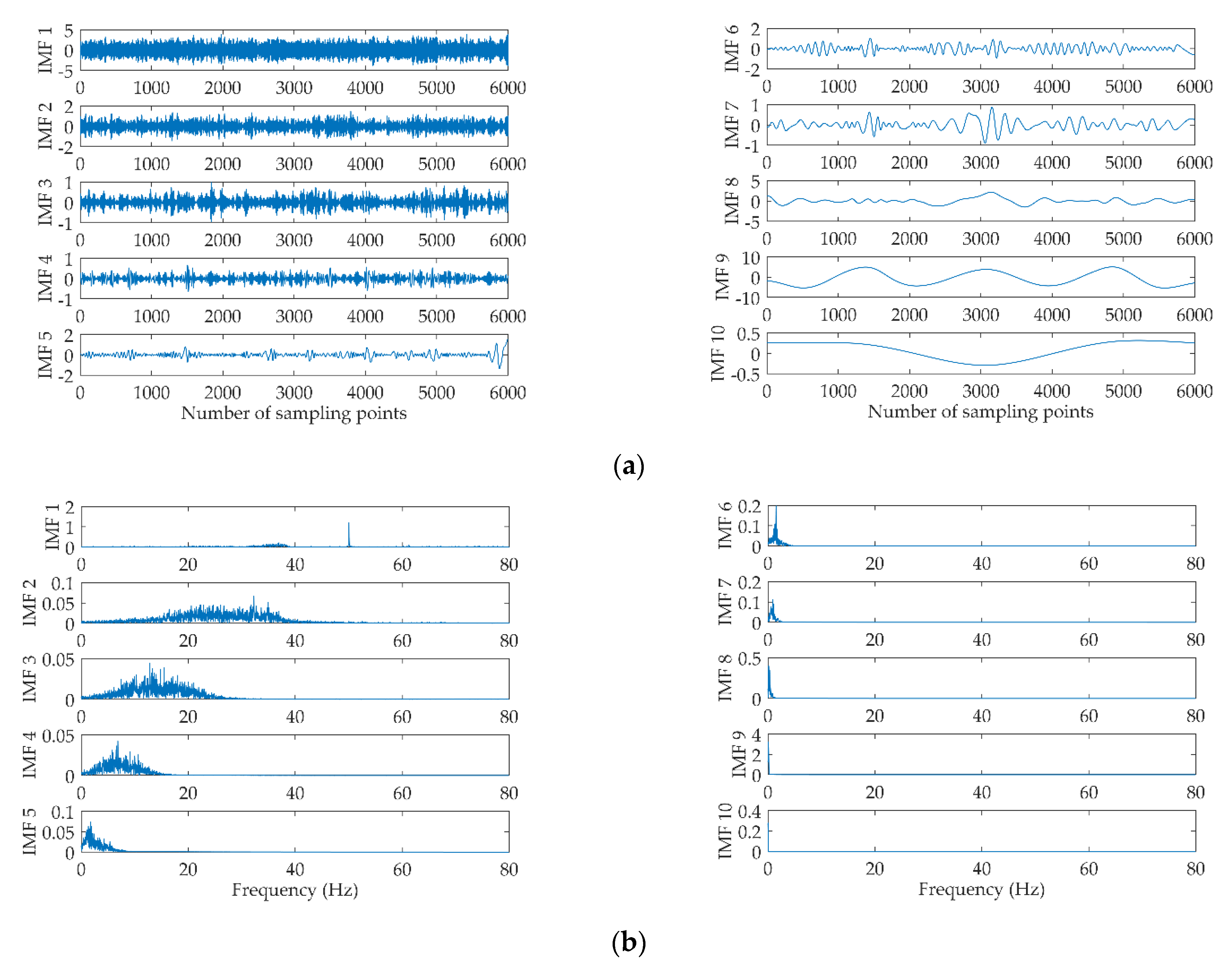
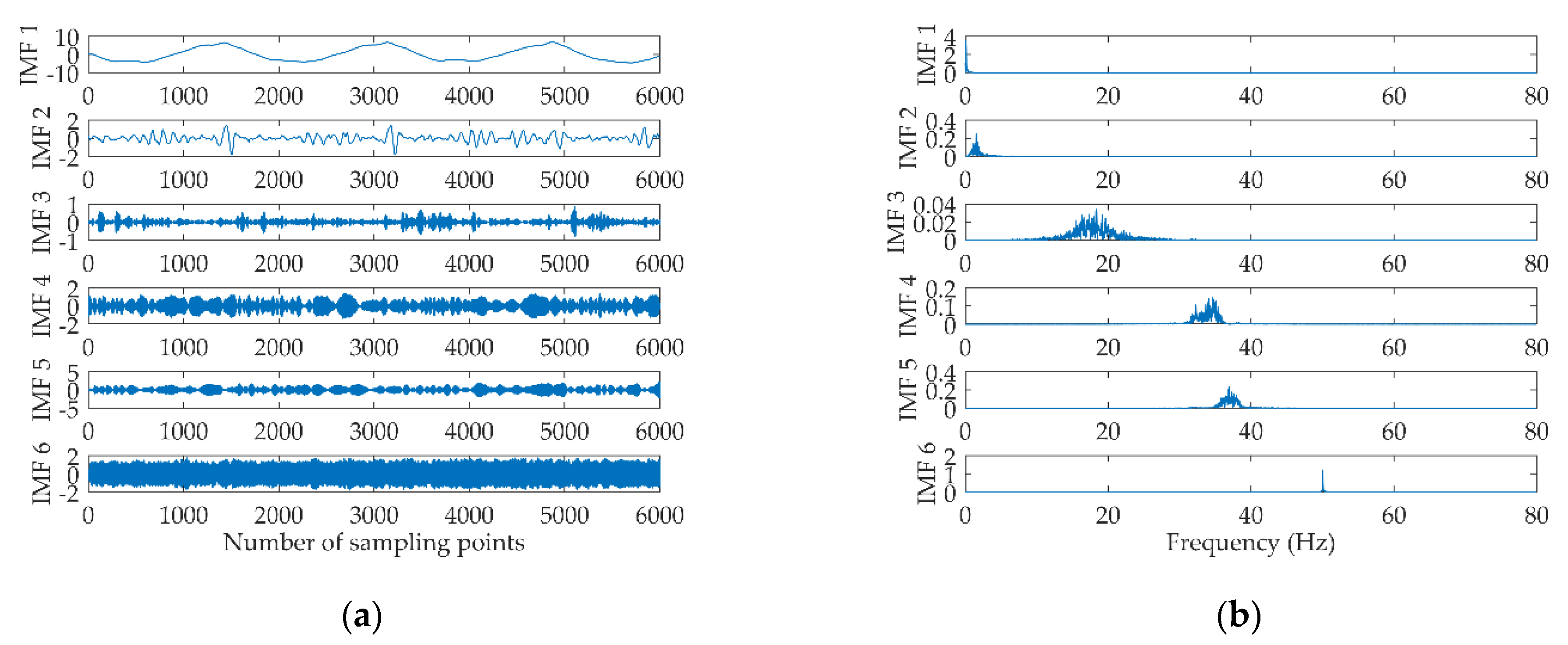
  • VMD can significantly reduce the number of IMFs, and each IMF has a relatively clear physical meaning.
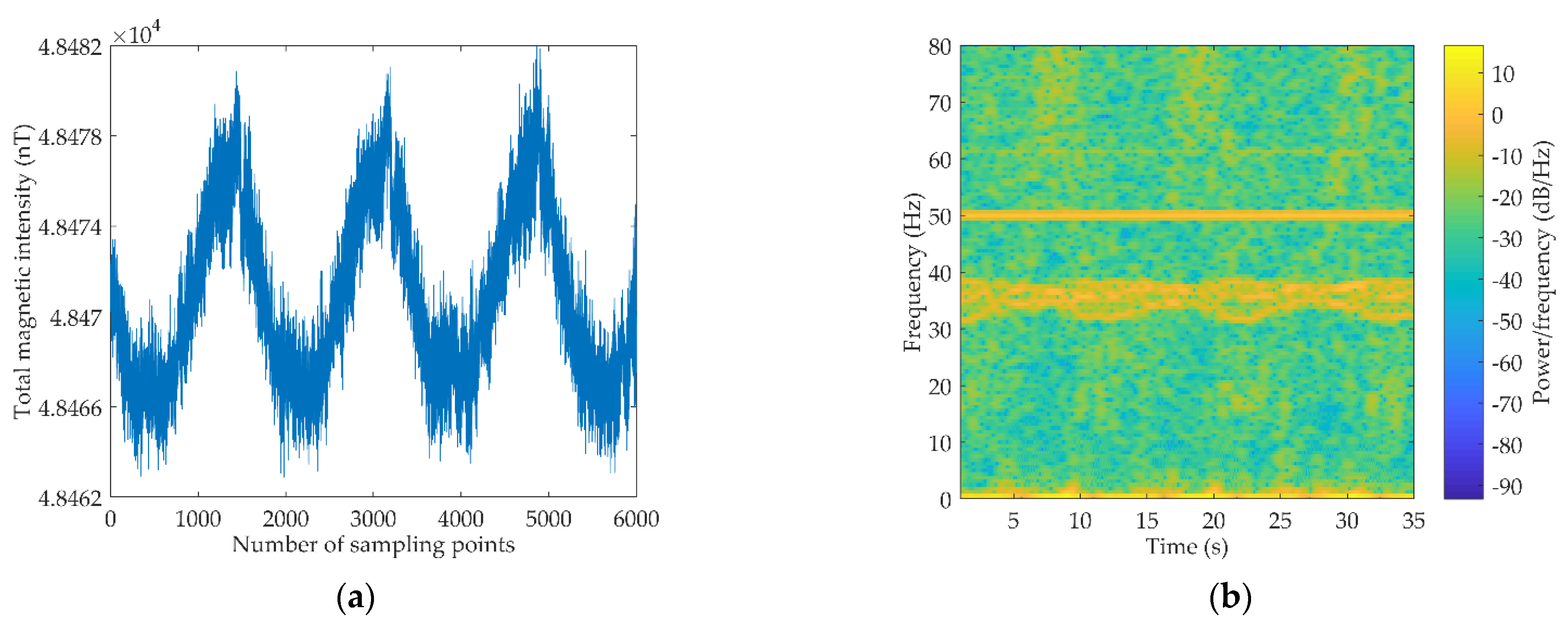
  • The center frequency of IMF1 is close to DC, which needs to be paid more attention to in the magnetic survey because the anomaly signal caused by the target is also quasi-static.
  • The energy of IMF2 is distributed in the frequency band of 0.5-3 Hz, which is the interference related to the maneuver of the UAV.
  • IMF3-IMF5 is the interference produced by the UAV platform, which may be related to the airborne electronic equipment.
  • The center frequency of IMF6 is 50 Hz, which is the power frequency interference.
To further verify the effectiveness of the proposed VMD method, a low-pass filter [14], an improved EMD method, and a complete ensemble empirical mode decomposition with adaptive noise (CEEMDAN) method [16], are used to process the original signal shown in Figure 3a. PE and the processing time are used as evaluation indicators, i.e., the smaller the PE is, the more obvious the interference suppression effect is; the shorter the processing time is, the better the real-time performance is. Results of PE and the processing time obtained by the four methods are given in Table 3. Although the proposed method is inferior to the low-pass filter and EMD-based method in processing time, it achieves the best effect of interference suppression. In addition, compared with the CEEMDAN method, the proposed method has shorter processing time, which means that it has better real-time performance.

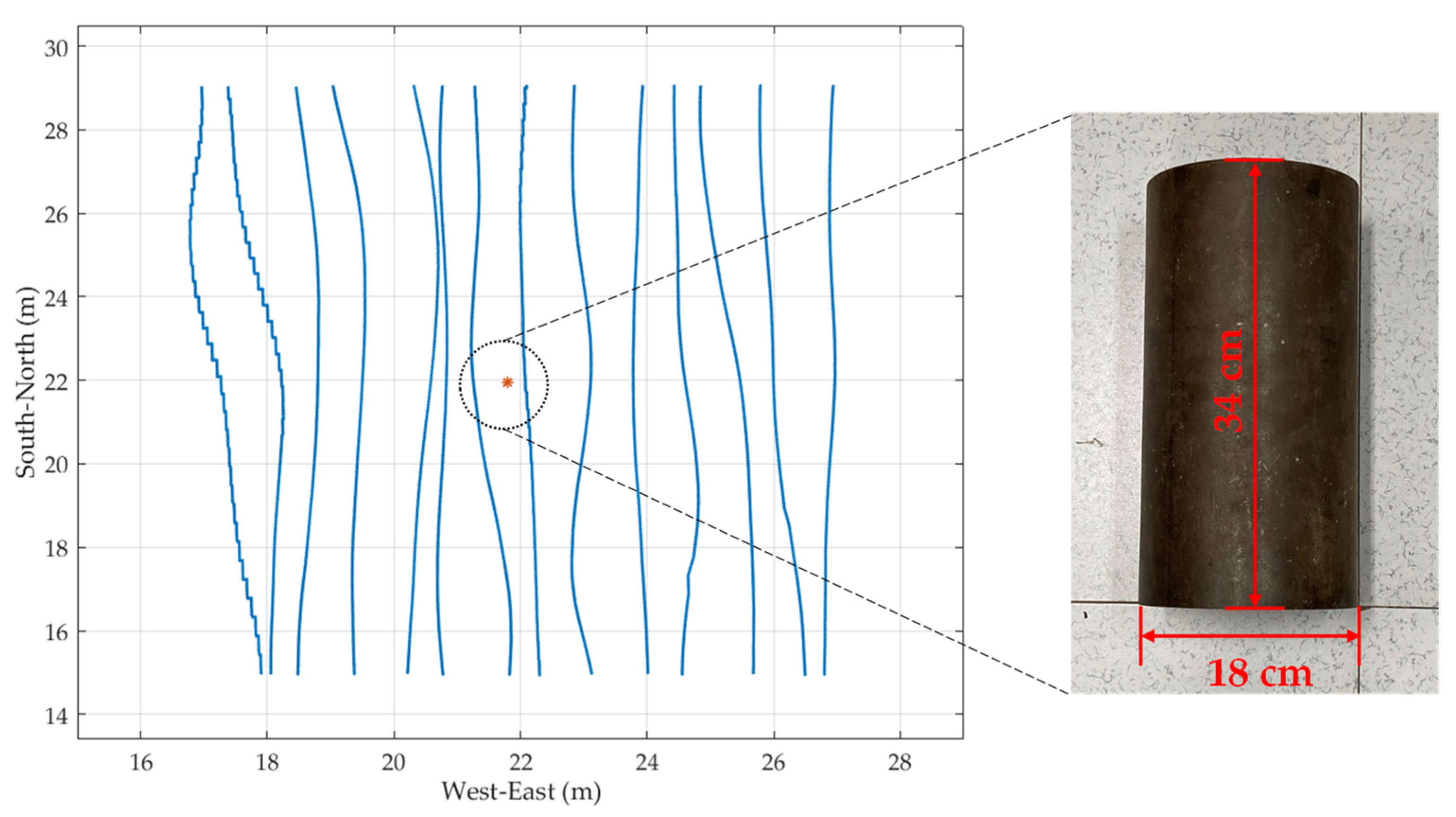
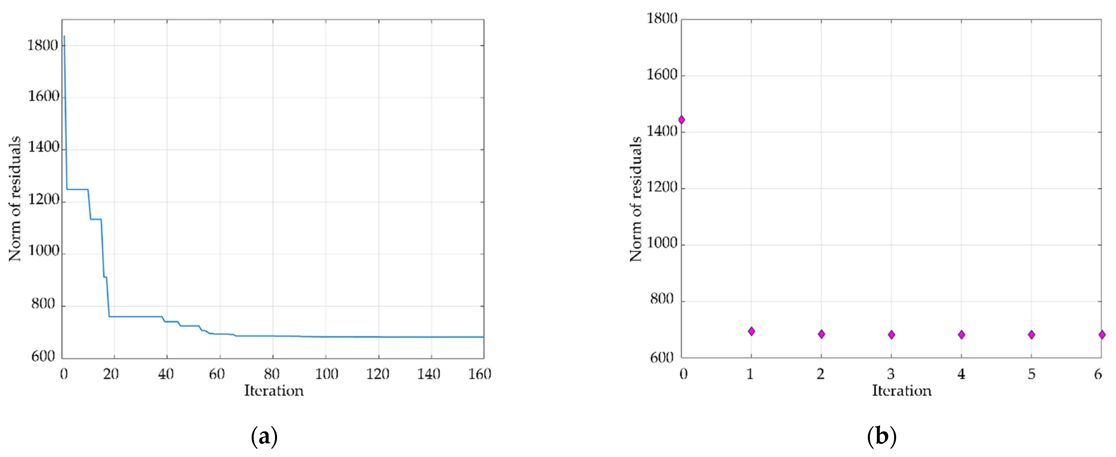
4.4. UAV Magnetic Data Interpretation

The field experiment was conducted in Hunan Province, China, on 12 October 2021. A cylindrical steel pipe is buried in the center of the survey area, with a depth of about 0.58 m. The pre-programmed flight profiles run along the north-south direction, with a line spacing of 0.75 m. The actual flight trajectory and the relative position of the target in the survey area are shown in Figure 6; due to the influence of crosswind, the actual line spacing is 0.2–1.2 m. The flight altitude of the UAV is 2 m, with an airspeed of about 2 m/s.
The magnetic map of the survey area obtained by the original data is shown in Figure 7a; the characteristics of the target are masked due to the low SNR of the original data. The proposed VMD-based method is applied to process the original data, then the magnetic map of the survey area is obtained by interpolating the processed data, as shown in Figure 7b. It can be clearly found that the quality of the processed data has been greatly improved compared with the original data, which lays a foundation for the further interpretation.
The magnetic anomaly area of Figure 7b is selected, then Euler deconvolution is used to obtain a preliminary estimate of the position and magnetic moment of the target. Finally, these parameters are taken as the initial values of the LM algorithm, and the further estimation of the parameters of the target is obtained. Table 4 shows the real position of the target and the estimated parameters obtained by the above two different methods, in which the real position of the target is obtained by the differential real-time kinematic (RTK) with centimeter-level accuracy. According to Table 4, the target position estimated by the joint Euler deconvolution-LM method is closer to the real value compared with the Euler deconvolution method, the horizontal positioning error is reduced from 15.31 cm to 4.05 cm, and the depth estimation error is reduced from 16.2 cm to 5.4 cm.
To further evaluate the convergence of the inversion model, the coefficient of determination (also known as R-squared) is introduced. By comparing the observed and predicted values of magnetic anomaly, R-squared can be defined as follows:
R 2 = 1 i ( B p r e d , i B o b s , i ) 2 i ( B p r e d , i B o b s ^ ) 2 ,
where i [ 1 , N ] , and N is the number of observed points. B o b s , i and B p r e d , i are the observed and predicted values of magnetic anomaly at the ith point, and B o b s ^ is the mean value of B o b s , i . By combining the Euler deconvolution and the LM algorithm, the value of R 2 reaches 0.9736, which is significantly better than the 0.8749 based on the Euler deconvolution method. It is proved that the proposed method can obtain more realistic inversion results, which is very important for further data interpretation.
Although some global optimization algorithms such as DE can also gain accurate estimation of the target parameters, these methods usually take more time than the joint Euler deconvolution-LM method proposed in this paper. Figure 8 shows the variation of the norm of residual error with iterations when using DE and the proposed method, respectively. For the sake of fairness, the search space of DE is set to be relatively compact, and its upper and lower bounds are x m a x = [23, 23, 1.2, 0.8, 0.8, 2] and x m i n = [21, 21, −0.5, −0.8, −0.8, −2], respectively. The population size is set to be 60, and the mutation scale factor F and the crossover rate CR are set to be 0.6 and 0.4, respectively.
As can be seen from Figure 8, the results of the two methods are very similar; the DE method obtains a stable solution after about 80 iterations, while the proposed method completes the process in less than 6 iterations. Under the same computer configuration, the DE method spends 46.69 s to complete the task; for comparison, the proposed method takes 1.39 s, which shows excellent efficiency.

5. Final Remarks

This paper presents a complete workflow for the processing and interpretation of UAV magnetic data, which mainly includes two parts: (1) UAV magnetic data processing based on the improved VMD method, in which the decomposition modes number K is adaptively determined by mode characteristics; and (2) UAV magnetic data interpretation based on Euler deconvolution and LM algorithm, where the target parameters are first estimated by Euler deconvolution, and then used as priori information of the LM algorithm. The results of field experiments show that the proposed method can be applied to UAV magnetic data processing, and the estimated target position is closer to the real situation.
In Section 4.3, the improved VMD method is applied to the UAV magnetic data processing. It is worth noting that, when the decomposition modes number K is appropriate, the result of VMD has a clear physical meaning, which is not available in other methods. We believe that this discovery is of great significance for the UAV magnetic interference mapping and suppression and is worthy of in-depth study. Section 4.4 establishes a step-by-step data interpretation method based on Euler deconvolution and LM algorithm, which makes full use of the local optimization and the fast convergence of the LM algorithm. The horizontal positioning error of the target is reduced to less than 10 cm, which is very beneficial to the follow-up work, such as the clearance of targets.
Nevertheless, there are some drawbacks in this paper. For example, this paper only optimizes the decomposition modes number K of VMD, and better results may be obtained by considering the influence of penalty factor α . Moreover, it should be noted that the proposed data interpretation method is only suitable for an isolated target, and if multiple targets exist or the distance between targets is very close, it is recommended to consider gradient or gradient tensor data [33,40]. In addition, due to the limited information of the collected magnetic anomaly data, more detailed parameters (e.g., shape, attitude, and material) of the target cannot be obtained. More comprehensive information about the target can be obtained by enriching sensor data, and there have been some successful attempts in this regard [41,42,43].
Our future work will focus on these issues, and mainly includes the following three parts: 1. Further optimize the VMD method to get better data processing results; 2. To improve the spatial resolution of the target through gradient measurement; 3. To obtain more abundant target parameters by combining other types of sensors (e.g., hyperspectral, electromagnetic) for data interpretation.

Supplementary Materials

The detailed parameters of the UAV magnetic system are available online at https://www.mdpi.com/1099-4300/23/10/1309/htm, Table 6: The technical specifications of the multi-rotor UAV magnetic survey system.

Author Contributions

Conceptualization, Y.Z. and X.Z.; methodology, Y.Z.; software, Y.Z.; validation, S.L., K.X. and Y.Z.; formal analysis, X.Z.; writing—original draft preparation, Y.Z.; writing—review and editing, X.Z.; visualization, S.L. and K.X.; supervision, X.Z.; funding acquisition, X.Z. All authors have read and agreed to the published version of the manuscript.

Funding

This research received no external funding.

Data Availability Statement

Data used during the study are available from the corresponding author by request.

Acknowledgments

The authors appreciate and thank Drones Assistant Editor Claudia Dragan, and anonymous reviewers for their warm work and valuable comments which helped to improve this manuscript.

Conflicts of Interest

The authors declare no conflict of interest.

References

  1. Yao, H.; Qin, R.; Chen, X. Unmanned Aerial Vehicle for Remote Sensing Applications—A Review. Remote Sens. 2019, 11, 1443. [Google Scholar] [CrossRef] [Green Version]
  2. Baji, M. Modeling and Simulation of Very High Spatial Resolution UXOs and Landmines in a Hyperspectral Scene for UAV Survey. Remote Sens. 2021, 13, 837. [Google Scholar] [CrossRef]
  3. Parshin, A.; Morozov, V.; Snegirev, N.; Valkova, E.; Shikalenko, F. Advantages of Gamma-Radiometric and Spectrometric Low-Altitude Geophysical Surveys by Unmanned Aerial Systems with Small Scintillation Detectors. Appl. Sci. 2021, 11, 2247. [Google Scholar] [CrossRef]
  4. Zheng, Y.; Li, S.; Xing, K.; Zhang, X. Unmanned Aerial Vehicles for Magnetic Surveys: A Review on Platform Selection and Interference Suppression. Drones 2021, 5, 93. [Google Scholar] [CrossRef]
  5. Hashimoto, T.; Koyama, T.; Kaneko, T.; Ohminato, T.; Yanagisawa, T.; Yoshimoto, M.; Suzuki, E. Aeromagnetic survey using an unmanned autonomous helicopter over Tarumae Volcano, northern Japan. Explor. Geophys. 2014, 45, 37–42. [Google Scholar] [CrossRef] [Green Version]
  6. Gailler, L.; Labazuy, P.; Régis, E.; Bontemps, M.; Souriot, T.; Bacques, G.; Carton, B. Validation of a new UAV magnetic prospecting tool for volcano monitoring and geohazard assessment. Remote Sens. 2021, 13, 894. [Google Scholar] [CrossRef]
  7. Luoma, S.; Zhou, X. Construction of a fluxgate magnetic gradiometer for integration with an unmanned aircraft system. Remote Sens. 2020, 12, 2551. [Google Scholar] [CrossRef]
  8. Fernandez Romero, S.; Morata Barrado, P.; Rivero Rodriguez, M.A.; Vazquez Yañez, G.A.; De Diego Custodio, E.; Michelena, M.D. Vector magnetometry using remotely piloted aircraft systems: An example of application for planetary exploration. Remote Sens. 2021, 13, 390. [Google Scholar] [CrossRef]
  9. Cunningham, M.; Samson, C.; Wood, A.; Cook, I. Aeromagnetic surveying with a rotary-wing unmanned aircraft system: A case study from a zinc deposit in Nash Creek, New Brunswick, Canada. Pure Appl. Geophys. 2018, 175, 3145–3158. [Google Scholar] [CrossRef]
  10. Schmidt, V.; Becken, M.; Schmalzl, J. A UAV-borne magnetic survey for archaeological prospection of a Celtic burial site. First Break. 2020, 38, 61–66. [Google Scholar] [CrossRef]
  11. Shahsavani, H. An aeromagnetic survey carried out using a rotary-wing UAV equipped with a low-cost magneto-inductive sensor. Int. J. Remote Sens. 2021, 42, 1–14. [Google Scholar] [CrossRef]
  12. Malehmir, A.; Dynesius, L.; Paulusson, K.; Paulusson, A.; Johansson, H.; Bastani, M.; Wedmark, M.; Marsden, P. The potential of rotary-wing UAV-based magnetic surveys for mineral exploration: A case study from central Sweden. Lead. Edge. 2017, 36, 552–557. [Google Scholar] [CrossRef]
  13. Walter, C.; Braun, A.; Fotopoulos, G. Spectral analysis of magnetometer swing in high-resolution UAV-borne aeromagnetic surveys. In Proceedings of the 2019 IEEE Systems and Technologies for Remote Sensing Applications Through Unmanned Aerial Systems (STRATUS), Rochester, NY, USA, 25–27 February 2019; pp. 1–4. [Google Scholar]
  14. Mu, Y.; Zhang, X.; Xie, W.; Zheng, Y. Automatic detection of near-surface targets for unmanned aerial vehicle (UAV) magnetic survey. Remote Sens. 2020, 12, 452. [Google Scholar] [CrossRef] [Green Version]
  15. Liu, D.; Xu, X.; Huang, C.; Zhu, W.; Liu, X.; Yu, G.; Fang, G. Adaptive cancellation of geomagnetic background noise for magnetic anomaly detection using coherence. Meas. Sci. Technol. 2014, 26, 015008. [Google Scholar] [CrossRef]
  16. Zheng, Y.; Li, S.; Xing, K.; Zhang, X. A Novel Noise Reduction Method of UAV Magnetic Survey Data Based on CEEMDAN, Permutation Entropy, Correlation Coefficient and Wavelet Threshold Denoising. Entropy 2021, 23, 1309. [Google Scholar] [CrossRef]
  17. Dragomiretskiy, K.; Zosso, D. Variational mode decomposition. IEEE Trans. Signal Process. 2013, 62, 531–544. [Google Scholar] [CrossRef]
  18. Liu, W.; Cao, S.; Chen, Y. Applications of variational mode decomposition in seismic time-frequency analysis. Geophysics 2016, 81, V365–V378. [Google Scholar] [CrossRef]
  19. Li, Y.; Li, Y.; Chen, X.; Yu, J. Denoising and feature extraction algorithms using NPE combined with VMD and their applications in ship-radiated noise. Symmetry 2017, 9, 256. [Google Scholar] [CrossRef] [Green Version]
  20. Ding, J.; Xiao, D.; Li, X. Gear fault diagnosis based on genetic mutation particle swarm optimization VMD and probabilistic neural network algorithm. IEEE Access. 2020, 8, 18456–18474. [Google Scholar] [CrossRef]
  21. Lahmiri, S.; Boukadoum, M. Biomedical image denoising using variational mode decomposition. In Proceedings of the 2014 IEEE Biomedical Circuits and Systems Conference (BioCAS) Proceedings, Lausanne, Switzerland, 22–24 October 2014; pp. 340–343. [Google Scholar]
  22. Wang, P.; Gao, Y.; Wu, M.; Zhang, F.; Li, G.; Qin, C. A denoising method for fiber optic gyroscope based on variational mode decomposition and beetle swarm antenna search algorithm. Entropy 2020, 22, 765. [Google Scholar] [CrossRef]
  23. Lian, J.; Liu, Z.; Wang, H.; Dong, X. Adaptive variational mode decomposition method for signal processing based on mode characteristic. Mech. Syst. Signal Proc. 2018, 107, 53–77. [Google Scholar] [CrossRef]
  24. Liu, L.; Chen, L.; Wang, Z.; Liu, D. Early fault detection of planetary gearbox based on acoustic emission and improved variational mode decomposition. IEEE Sens. J. 2020, 21, 1735–1745. [Google Scholar] [CrossRef]
  25. Hinze, W.J.; Von Frese, R.R.; Von Frese, R.; Saad, A.H. Gravity and Magnetic Exploration: Principles, Practices, and Applications; Cambridge University Press: Cambridge, UK, 2013; pp. 338–411. [Google Scholar]
  26. Reid, A.B.; Allsop, J.; Granser, H.; Millett, A.t.; Somerton, I. Magnetic interpretation in three dimensions using Euler deconvolution. Geophysics 1990, 55, 80–91. [Google Scholar] [CrossRef] [Green Version]
  27. Mushayandebvu, M.F.; van Driel, P.; Reid, A.B.; Fairhead, J.D. Magnetic source parameters of two-dimensional structures using extended Euler deconvolution. Geophysics. 2001, 66, 814–823. [Google Scholar] [CrossRef]
  28. Keating, P.; Pilkington, M. Euler deconvolution of the analytic signal and its application to magnetic interpretation. Geophys. Prospect. 2004, 52, 165–182. [Google Scholar] [CrossRef]
  29. Davis, K.; Li, Y.; Nabighian, M. Automatic detection of UXO magnetic anomalies using extended Euler deconvolution. Geophysics 2010, 75, G13–G20. [Google Scholar] [CrossRef]
  30. Zhou, Z.; Zhang, M.; Chen, J. A new multiple magnetic targets location method in 3D space. In SEG Technical Program Expanded Abstracts 2020; Society of Exploration Geophysicists: Tulsa, OK, USA, 2020; pp. 974–978. [Google Scholar]
  31. Huang, L.; Zhang, H.; Sekelani, S.; Wu, Z. An improved Tilt-Euler deconvolution and its application on a Fe-polymetallic deposit. Ore Geol. Rev. 2019, 114, 103114. [Google Scholar] [CrossRef]
  32. Ma, G.-Q.; Yong, X.-Y.; Li, L.-L.; Guo, H. Three-dimensional gravitational and magnetic-data acquisition and analysis via a joint-gradient Euler-deconvolution method. Appl. Geophys. 2020, 17, 297–305. [Google Scholar] [CrossRef]
  33. Ding, X.; Li, Y.; Luo, M.; Chen, J.; Li, Z.; Liu, H. Estimating Locations and Moments of Multiple Dipole-Like Magnetic Sources From Magnetic Gradient Tensor Data Using Differential Evolution. IEEE Trans. Geosci. Remote Sens. 2021. [CrossRef]
  34. Marquardt, D.W. An algorithm for least-squares estimation of nonlinear parameters. J. Soc. Ind. Appl. Math. 1963, 11, 431–441. [Google Scholar] [CrossRef]
  35. Madsen, K.; Nielsen, H.B.; Tingleff, O. Methods for Non-Linear Least Squares Problems; Informatics and Mathematical Modelling, Technical University of Denmark: Copenhagen, Denmark, 2004. [Google Scholar]
  36. Börlin, N.; Grussenmeyer, P. Bundle adjustment with and without damping. Photogramm. Rec. 2013, 28, 396–415. [Google Scholar] [CrossRef] [Green Version]
  37. Li, Y.; Chen, X.; Yu, J.; Yang, X.; Yang, H. The data-driven optimization method and its application in feature extraction of ship-radiated noise with sample entropy. Energies 2019, 12, 359. [Google Scholar] [CrossRef] [Green Version]
  38. Song, Q.; Ding, W.; Peng, H.; Gu, J.; Shuai, J. Pipe defect detection with remote magnetic inspection and wavelet analysis. Wirel. Pers. Commun. 2017, 95, 2299–2313. [Google Scholar] [CrossRef]
  39. Sheinker, A.; Shkalim, A.; Salomonski, N.; Ginzburg, B.; Frumkis, L.; Kaplan, B.-Z. Processing of a scalar magnetometer signal contaminated by 1/fα noise. Sens. Actuators A Phys. 2007, 138, 105–111. [Google Scholar] [CrossRef]
  40. Gang, Y.; Yingtang, Z.; Hongbo, F.; Zhining, L.; Guoquan, R. Detection, localization and classification of multiple dipole-like magnetic sources using magnetic gradient tensor data. J. Appl. Geophys. 2016, 128, 131–139. [Google Scholar] [CrossRef]
  41. Jackisch, R.; Madriz, Y.; Zimmermann, R.; Pirttijärvi, M.; Saartenoja, A.; Heincke, B.H.; Salmirinne, H.; Kujasalo, J.-P.; Andreani, L.; Gloaguen, R. Drone-borne hyperspectral and magnetic data integration: Otanmäki Fe-Ti-V deposit in Finland. Remote Sens. 2019, 11, 2084. [Google Scholar] [CrossRef] [Green Version]
  42. Mu, Y.; Xie, W.; Zhang, X. The Joint UAV-Borne Magnetic Detection System and Cart-Mounted Time Domain Electromagnetic System for UXO Detection. Remote Sens. 2021, 13, 2343. [Google Scholar] [CrossRef]
  43. Parshin, A.; Bashkeev, A.; Davidenko, Y.; Persova, M.; Iakovlev, S.; Bukhalov, S.; Grebenkin, N.; Tokareva, M. Lightweight unmanned aerial system for time-domain electromagnetic prospecting—the next stage in applied UAV-Geophysics. Appl. Sci. 2021, 11, 2060. [Google Scholar] [CrossRef]
Figure 1. The proposed workflow for the processing and interpretation of UAV magnetic data.
Drones 06 00011 g001
Figure 2. The six-rotor-based UAV magnetic survey system.
Drones 06 00011 g002
Figure 3. (a) The original data; (b) The time-frequency spectrogram of the original data after DC component removed.
Drones 06 00011 g003
Figure 4. (a) The 10 IMFs obtained by EMD; (b) The corresponding spectrum of the 10 IMFs.
Drones 06 00011 g004
Figure 5. (a) The 6 IMFs obtained by VMD; (b) The corresponding spectrum of the 6 IMFs.
Drones 06 00011 g005
Figure 6. Flight profiles of the drone; the red ‘ * ’ indicates the location of the target.
Drones 06 00011 g006
Figure 7. Magnetic map of the survey area obtained by (a) the original data and (b) the processed data using VMD-based method, the unit of magnetic field in both figures is nano Tesla.
Drones 06 00011 g007
Figure 8. The variation of the norm of residual error with iterations when using (a) DE algorithm and (b) the proposed method.
Drones 06 00011 g008
Table 1. The center frequencies of IMFs and the energy loss coefficient with different K.
KCenter Frequency/HzEnergy Loss Coefficient
41.4534.4537.32 0.2534
51.4318.8134.4937.74 0.2469
61.4117.8634.0236.9950.04 0.0980
71.4117.6332.3735.0937.2750.040.0939
Table 2. The correlation coefficients between the new IMF and the previous IMFs.
KNew IMFCorrelation Coefficients
5IMF 30.00310.02620.04740.0294
6IMF 60.00130.01130.07830.11030.0821
7IMF 40.00040.00300.04180.63270.08320.0039
Table 3. PE and the processing time obtained by the four different methods.
MethodLow-Pass FilterEMDCEEMDANProposed
PE0.43620.44140.39660.3091
Processing time/s0.1121.00810.1454.305
Table 4. Results of estimated target parameters obtained by two methods.
ParameterRealEuler-DeconvolutionJoint Euler-LM Method
Location (m)(21.802, 21.964, −0.580)(21.806, 22.117, −0.742)(21.791, 21.925, −0.526)
Magnetic moment (Am2)-(−0.044, 0.534, −1.113)(−0.106, 0.630, −1.235)
Publisher’s Note: MDPI stays neutral with regard to jurisdictional claims in published maps and institutional affiliations.

