Convolutional Neural Networks for Classification of Drones Using Radars

Abstract

The ability to classify drones using radar signals is a problem of great interest. In this paper, we apply convolutional neural networks (CNNs) to the Short-Time Fourier Transform (STFT) spectrograms of the simulated radar signals reflected from the drones. The drones vary in many ways that impact the STFT spectrograms, including blade length and blade rotation rates. Some of these physical parameters are captured in the Martin and Mulgrew model which was used to produce the datasets. We examine the data under X-band and W-band radar simulation scenarios and show that a CNN approach leads to an ${\mathrm{F}}_1$ score of $0.816\pm 0.011$ when trained on data with a signal-to-noise ratio (SNR) of 10 dB. The neural network which was trained on data from an X-band radar with 2 kHz pulse repetition frequency was shown to perform better than the CNN trained on the aforementioned W-band radar. It remained robust to the drone blade pitch and its performance varied directly in a linear fashion with the SNR.

1. Introduction

Modern drones are more affordable than ever, and their uses extend into many industries such as emergency response, disease control, weather forecasting, and journalism [1]. Their increased military use and the possible weaponization of drones have caused drone detection and identification to be an important matter of public safety.

There are several types of technology which can facilitate drone detection and classification. Some sensors employ sound-based or acoustic technology to classify drones. Drones give off a unique acoustic signature ranging from 400 Hz to 8 kHz, and microphones can capture this information. Unfortunately, this technology can only be used at a maximum range of 10 meters, and the microphones are sensitive to environmental noise [2]. When tracking drones through the air, this method becomes impractical.

Optical sensors use one or more cameras to create a video showing the target drone. The classification problem then becomes the identification of specific patterns in the shapes and colours of the drones. This approach is a popular technique because it is intuitive and enables the use of image processing and computer vision libraries [3] as well as neural networks [4]. However, optical sensors have a limited range and require favourable weather conditions. For these reasons, they are not reliable enough to use for drone classification, especially at longer ranges.

Drones and other unmanned aerial vehicles (UAVs) rely on (typically hand-held) controllers, which send radio frequency signals to the drone. These signals have a unique radio frequency fingerprint that depends on the circuitry of the controller, drone, and the chosen modulation techniques. Radio frequency fingerprint analysis has been studied as a method to detect and classify drones [5].

Finally, radar sensors for drone tracking and classification have been extensively studied [6,7,8,9]. Radars are capable of detecting targets at longer ranges than other sensors and perform reliably in all weather conditions at any time of day [10].

The classification technique investigated in this paper is based on the target drone’s micro-Doppler signature. A micro-Doppler signature is created when specific components of an object move separately from the rest. The rotation of propeller blades on a drone is sufficient to generate these signatures. The use of radars for studying micro-Doppler signatures has been shown effective [11] and has been used in conjunction with machine learning for many UAV classification problems [12,13,14,15,16,17,18,19]. As such, radars are the chosen technology for this paper.

Previous work has shown that an analysis of the radar return, including the micro-Doppler signature, can reliably distinguish drones from birds [7,8,20]. We now turn to the problem of distinguishing different types of drones. Standard analyses of the radar return include using the short-window and long-window Short Time Fourier Transform (STFT). The short- and long- window labels refer to the rotation period of the drone, or the time it takes for the drone’s blades to make a complete 360-degree rotation. A short-window STFT is when the window length is less than a rotation period, while a long-window STFT is when the window length exceeds the rotation period. The long-window STFT generates a unique signature of the drones in the form of Helicopter Rotation Modulation (HERM) lines. The number of HERM lines and their frequency separation can be used to distinguish between the different drones.

For situations where the pulse repetition frequency (PRF) of the radar is not high enough to extract the full micro-Doppler signature, Huang et al. proposed a log harmonic summation algorithm to use on the HERM lines [21]. This algorithm estimates the micro-Doppler periodicity and performs better than the previously used cepstrum method [8] in the presence of noise. Huang also showed using collected radar data that the Minimum Description Length Parametric Spectral Estimation Technique reliably estimates the number of HERM lines. This information can be used to determine whether the target is a rotary drone with spinning propellers [22].

When the full micro-Doppler signature is available (using a high PRF radar), the short-window STFT can be utilized for analysis. Klaer et al. used HERM lines to estimate the number of propeller blades in these situations [23]. They also proposed a new multi-frequency analysis of the HERM lines, which enables the approximation of the propeller rates [23]. In this paper, we leverage the work of Hudson et al., who demonstrated the potential of passing STFT spectrograms into a Convolutional Neural Network (CNN) to classify drones [13].

Recently, Passafiume et al. presented a novel micro-Doppler vibrational spectral model for flying UAVs using radars. This model incorporates the number of vibrational motors in the drone and the propeller rotation rates. They showed that this model is able to reliably simulate the micro-Doppler signature of drones. Furthermore, they proposed that the model could be further studied for use in unsupervised machine learning [24].

In another study, Lehmann and Dall trained a Support Vector Machine (SVM) on simulated data. They simulated their data by considering the drone as a set of point scatterers and superimposing the radar return of each point [25]. However, their work modelled the data as free from thermal noise. Using the Martin and Mulgrew model instead, we can simulate varying signal-to-noise ratio (SNR) conditions in this paper. Doing so provides a more realistic situation in which to apply machine learning. Additionally, our use of CNN provides better classification accuracy than their SVM.

In our investigation, we use the updated versions of the Martin and Mulgrew model [26] to simulate drone signals and perform additional augmentation to improve the data’s realism. We used the model to produce datasets distinguished by the SNR and PRFs of the contained samples. A CNN was trained for each of these datasets, and their performances were analyzed with the ${\mathrm{F}}_1$ metric. Our findings suggest that it is possible to train a robust five-drone classifier (plus an additional noise class) using just one thousand data samples, each 0.3 s in duration. Furthermore, we show it is possible to train CNN classifiers robust to SNR-levels not included in training while maintaining performance that is invariant to the blade pitch of the drones.

The work presented in this paper contributes to the field of drone classification in several ways. Many studies explore the use of neural networks for a specific SNR. Here, we provide an analysis for a wide range of SNR values, thus making our results more generalizable to different situations. We also show that the selected model is robust against varying pitches of the propeller blades, maintaining its performance when tested on drones whose blade pitch is outside of the training range. Additionally, we find that X-band radars provide better data than W-band radars for this application within the studied SNR range. This last result is likely due to the configuration of our neural network and may not be true in general cases. Finally, we leverage the Martin and Mulgrew model for data simulation, a model that is not commonly used for drone classification.

This paper is organized as follows. Section 2 introduces the reader to the concepts used in our work. We review some of the important radar parameters in Section 2.1, paying close attention to their use in our context. The Martin and Mulgrew model is used to simulate returns from different types of radars and is summarized in Section 2.2. Drone parameters and data generation are discussed in Section 2.3, and an overview of the machine learning pipeline is presented in Section 2.4. The results of the machine learning model are shown and discussed in Section 3 and Section 4, respectively. Finally, we present our conclusions and future steps in Section 5.

2. Materials and Methods

2.1. Radar Preliminaries

As discussed previously, radar (RAdio Detection And Ranging) systems are advantageous over other surveillance systems for several reasons. This subsection will define the radar parameters and discuss the signal-to-noise ratio and the radar cross-section, two significant quantities for drone classification.

2.1.1. Radar Parameters

There are two main classes of radars: active and passive. Active radars emit electromagnetic waves at the radio frequency and detect the pulse’s reflection off of objects. Passive radars detect reflections of electromagnetic waves that originated from other sources or other transmitters of opportunity. In this paper, we will be focusing our attention on active radars. Such radars may be either pulsed or frequency modulated continuous wave (FMCW) radars. Pulse radars transmit pulses at regular intervals, with nominal pulse duration (or pulse width) of the order of a micro-second and pulse repetition interval of the order of a millisecond. Many variables related to the radar and target dictate a radar’s performance. These variables are presented in

Table 1. The radar parameters and pre-determined quantities which describe the radar-drone interaction.

Symbol	Parameter Name and Interpretation
PRF	Pulse repetition frequency—The number of pulses emitted by the transmitting antenna every second in pulsed radars
SRF	Sweep repetition frequency—The number of sweeps emitted by the transmitting antenna every second in FMCW radars
$P_t$	Transmitter power—The power of the transmitted signal in Watts
$G_t$	Transmitting antenna gain—The gain of the transmitting antenna compared to an isotropic antenna [27]
$G_r$	Receiving antenna gain—The gain of the receiving antenna compared to an isotropic antenna. The radars simulated in this paper are monostatic radars, meaning that there is just one antenna for transmitting and receiving. Hence, $G_t=G_r$
$\lambda$	Wavelength—The wavelength of the light in the emitted pulse
$\sigma$	Radar cross-section (RCS)—The surface area of the target that is “visible” to the radar. More technically, it is defined as the surface area of a metal sphere which reflects the same amount of power as the object does [10]
$\tau$	Pulse width—The width or duration of the pulses in pulsed radar or sweep duration in FMCW radar
R	Range—the distance from the radar to the target
$T_n$	Noise temperature—The combined temperature of external radiating sources, thermal energy lost in the receiving/transmitting lines, and any internal receiver noise [27]
$k_b$	Boltzmann’s constant—The product $T_n\times k_b$ yields the power density in Watts per hertz of bandwidth that is lost due to temperature noise [27]
L	Loss—The loss incurred by transmission lines, an imperfect antenna, and the propagation medium (the air) [27]

.

For more information about radar types and their operations, we direct interested readers to the text by Dr. Skolnik [28]. We will now turn our attention to some of the specific measurements that help describe how radars can detect and classify drones.

2.1.2. Radar Cross-Section

The radar cross-section (RCS) is critical when working with drones. As explained in Table 1, the RCS of a target is the surface area that is visible to the radar. The RCS varies with the target’s size, shape, surface material, and pitch. Typical drones have an RCS value from −$15\mathrm{dBsm}$ to −$20\mathrm{dBsm}$ for X-band frequencies and smaller than −$20\mathrm{dBsm}$ for frequencies between 30–37$\mathrm{GHz}$ [29]. The RCS of drones varies significantly with the drone model and position in the air. A comprehensive study of drone RCS was performed by Shröder et al. They reported that the material is a significant factor in the blade RCS as metal blades have a much higher RCS than plastic ones [30].

The strength of the returned radar signal varies directly with the RCS, making it a critical factor in drone classification using radars. This paper will utilize the micro-Doppler effects from drone propeller blades. Thus, the RCS of the drones’ blades is much more important for this investigation than that of the body.

2.1.3. Signal-to-Noise Ratio

Another important quantity for radar studies is the signal-to-noise ratio (SNR). The SNR measures the ratio of received power from the target(s) and the received power from noise. The expression for the SNR depends on the radar parameters previously introduced, including the RCS, and is provided by the radar range equation [31]:

$$\mathrm{SNR}=\frac{P_t{G}_t{G}_r{\lambda }^2\sigma \tau }{{\left(4\pi \right)}^3{R}^4{T}_n{k}_{b}L}$$

(1)

One would expect that classification performance decreases with the SNR because the target becomes less clear. Dale et al. showed this to be true when distinguishing drones from birds [32]. As seen in Equation (1), the SNR is directly related to the RCS and so consequently tends to be small for drones. It is, therefore, crucial to understand and appreciate the signal SNR because it will significantly impact the quality of the trained model. If the training data has an SNR that is too high, the model will not generalize well to realistic scenarios with a lower SNR. The work later in this paper analyzes model performance as a function of the SNR of the signals in the training data.

It is often more convenient to express Equation (1) in decibels (dB), which is a logarithmic scale. The log-scale simplifies the calculation of the SNR quantity by adding the decibel equivalents of the numerator terms and subtracting those in the denominator. A Blake Chart clarifies this process.

Table 2. Example usage of a Blake Chart for calculating the SNR of a particular drone using a given radar.

Parameter	$\mathbf{Unit}\mathbf{Value}$	+ (dB)	− (dB)
Peak Power (W)	1 W	0	0
Gain (dB)	25 dB	50	0
Wavelength (m)	0.03 m	−30.464	0
Cross Section (m${}^2$)	0.01 m${}^2$	−20	0
Range (m)	1000 m	0	120.0
1/$k_b$ (m${}^{-2}$ · kg${}^{-1}$ · s${}^2$ · K)	1.380649e−23	228.599	0
System Temperature (K)	290 K	0	24.624
Pulse Width (s)	0.001 s	−30	0
${\left(4\pi \right)}^3$	1984.402	0	32.976
Losses (dB)	7 dB	0	7
Totals		198.135	−184.6
SNR Per Pulse		13.535 dB

shows an example of such a calculation where the radar operates in the X-band (10 GHz frequency) and the object is 1 km away.

Blake Charts make it easy to see how slightly adjusting one parameter can impact the SNR per pulse. It is important to note that for a particular radar and object at a specified range, the only parameters that can be adjusted are the $P_t,\lambda$, and $\tau$. Each of these parameters comes with an associated cost due to limited power supply or the specifications of the radar, and so it is not always possible to achieve a desirable SNR. Due to this, classification models need to perform well in low-SNR conditions.

2.2. Modelling Radar Returns from Drones

The Martin and Mulgrew equation models the complex radar return signal of aerial vehicles with rotating propellers [26]. The model assumes that the aerial vehicle (or drone in our context) has one rotor. The formulation of the model is presented in Equation (2) and was used to simulate radar return signals of five different drones under two different radar settings. French [33] provides a derivation and detailed insights on the model.

$$\psi \left(t\right)=A_r{e}^{j\left(2\pi f_{c}t-\frac{4\pi }{\lambda }\left(R+v_{\mathrm{rad}}t\right)\right)}\sum _{n=0}^{N-1}\left(\alpha +\beta cos{\Omega }_n\right)e^{-j\frac{L_1+L_2}{2}{\gamma }_n}\sin \mathrm{c}\left(\frac{L_2-L_1}{2}{\gamma }_n\right)$$

(2)

where

$$\begin{array}{cc}\hfill \alpha & =sin\left(\left|\theta \right|+{\varphi }_p\right)+sin\left(\left|\theta \right|-{\varphi }_p\right)\hfill \end{array}$$

(3)

$$\begin{array}{cc}\hfill \beta & =\mathrm{sign}\left(\theta \right)\left(sin\left(\left|\theta \right|+{\varphi }_p\right)-sin\left(\left|\theta \right|-{\varphi }_p\right)\right)\hfill \end{array}$$

(4)

$$\begin{array}{cc}\hfill {\Omega }_n& =2\pi \left(f_{r}t+\frac{n}{N}\right)\hfill \end{array}$$

(5)

$$\begin{array}{cc}\hfill {\gamma }_n& =\frac{4\pi }{\lambda }cos\theta sin{\Omega }_n\hfill \end{array}$$

(6)

Table 3. Interpretation of all the parameters in the Martin and Mulgrew model. $f_c$ and $\lambda$ depend on the specific radar. $\theta$, R, and $v_{\mathrm{rad}}$ depend on the position of the drone, while $f_r$, N, $L_1$, and $L_2$ are characteristic of the drone’s blades.

Parameter	Interpretation
$A_r$	Real valued scalar, the scale factor
t	Time
$f_c$	Frequency of the transmitted signal
$\lambda$	Wavelength of the transmitted signal
$\theta$	Angle between the target’s plane of rotation and the line of sight from the radar to the target’s center of rotation
R	Range of the target
$v_{\mathrm{rad}}$	Radial velocity of the target with respect to the radar
N	Number of propeller blades on target
$f_r$	Frequency of rotor rotation
$L_1$	Distance of the blade roots from the target’s centre of rotation
$L_2$	Distance of the blade tips from the target’s centre of rotation
${\varphi }_p$	Pitch of the blades relative to horizontal

provides a complete description of each of the parameters within the model. Excluding time, t, the model has eleven parameters approximately categorized as radar and drone parameters. Radar parameters include the carrier frequency, $f_c$, and the transmitted wavelength, $\lambda$. The latter set of parameters depends on the position of the drone relative to the radar and the characteristics of the drone’s propeller. In particular, the strength of the presented model over the initial version of the Martin and Mulgrew equation is its ability to account for variation in blade pitch of the drones, ${\varphi }_p$ [26,34].

For several reasons, the Martin and Mulgrew model was the chosen data simulation model. It is a model based on electromagnetic theory and Maxwell’s equations. Despite this, it is computationally efficient compared to more sophisticated models. Additionally, the drone parameters used were previously compiled and demonstrated by Hudson et al. [13]. The following section of this paper will strengthen confidence in the model by comparing it to an actual drone signal. It is found that the Martin and Mulgrew model produces distinct HERM line signatures (dependant on the parameters), as seen in the collected data—a fact that is crucial for this investigation. Although the number of rotors on the drone is not the focus of this paper, it is helpful to note that the model assumes that there is a single rotor. A proposed extension to the model sums the signal over the different rotors [35], but it has not been extensively studied.

2.3. Data Generation and Augmentation

This section describes the different sampling and augmentation considerations taken to simulate a Martin and Mulgrew signal. As will be elaborated in Section 2.4, many simulated signals were put together to produce datasets for machine learning.

The data simulation step involved two sets of radar parameters, representing an X-band and W-band radar, respectively. Furthermore, five sets of drone parameters corresponding to different commercial drones were used.

Table 4. Transmission wavelength and frequency values for a W-band and X-band radar.

Radar	$\mathit{\lambda }$ (cm)	${\mathit{f}}_{\mathit{c}}$ (GHz)
W-band	0.32	94.00
X-band	3.00	10.00

and

Table 5. Approximate drone-blade parameters of five drones.

Drone	N	${\mathit{L}}_1$ (cm)	${\mathit{L}}_2$ (cm)	${\mathit{f}}_{\mathit{r}}$ (Hz)
DJI Mavic Air 2	2	0.50	7.00	91.66
DJI Mavic Mini	2	0.50	3.50	160.00
DJI Matrice 300 RTK	2	5.00	26.65	70.00
DJI Phantom 4	2	0.60	5.00	116.00
Parrot Disco	2	1.00	10.40	40.00

have the parameters for the radars and drones’ blades. Note that along with the five drones (classes), a sixth Gaussian-noise class was produced to investigate the possibility of false alarms during classification and their impact.

Although the selected drones have fixed blade pitches, the parameter was assumed to be variable for modelling purposes since some drones can have adjustable blade pitches. This assumption can improve the generalizability of the analysis. Moreover, $\theta$ and R were similarly considered as variable parameters while $v_{\mathrm{rad}}$ and $A_r$ were set to be constant (zero and four, respectively) for simplicity. As seen in

Table 6. Sampling distributions for some variable parameters.

Variable Parameter	Distribution
${\varphi }_p$ (rad)	$\sim \mathcal{U}$(0, $\pi /4$)
$\theta$ (rad)	$\sim \mathcal{U}$($\pi /16$, $\pi /2$)
R (m)	$\sim \mathcal{U}$(500, 2000)
$v_{\mathrm{rad}}$ (rad/s)	Asserted to be 0
$A_r$	Asserted to be 4

, these variable parameters were uniformly sampled to produce meaningful variations between each simulated drone signal.

Besides varying the above parameters, additional methods were used to produce differences between the simulated signals. We applied shifts in the time domain, adjusted the signal to reflect the probability of detection, and added noise to augment each sample. The time shift was introduced by randomly selecting a $t_s$ such that the resulting signal would be $\psi (t+t_s)$. Next, a probability of detection ($p_d$) of $0.8$ was asserted by removing some data from the signal, simulating the amount of information typically present in real scenarios. Finally, Gaussian-normal noise was introduced to produce a signal of the desired SNR. The added noise, $\mathbf{n}$, was sampled from $\mathcal{N}(0,{\sigma }_0)$ where the standard deviation was given by the rearranged form of Equation (7). Equation (8) presents the final augmented signal produced using the Martin and Mulgrew equations. Each simulated sample used for machine learning was $0.3$ s in length.

$$\mathrm{SNR}=10{log}_{10}\left(\frac{A_r^2}{{\sigma }_0^2}\right)\leftarrow \stackrel{\mathrm{rearranged}}{\to }{\sigma }_0=\sqrt{{10}^{-\mathrm{SNR}/10}{A}_r^2}$$

(7)

$${\psi }_{\mathrm{final}}\left(t\right)=\mathrm{detection}\left(\psi \left(t+t_s\right),p_d=0.8\right)+\mathbf{n}$$

(8)

The use of a convolutional network requires data with spatially relevant information. The long-window STFT was applied to produce a spectrogram representation of the simulated signals [36]. The STFT is one of many methods used to produce spectrograms for convolutional learning [18]. Recall that a short-window STFT has a window size smaller than the rotation period of the drone. However, according to the Nyquist Sampling Theorem, using a short window requires that the radar PRF is at least four times the maximum Doppler shift of the propeller blades to detect micro-Doppler blade flashes unambiguously. In contrast, a long-window STFT cannot detect blade flashes because the window size is larger than the rotational period of the propellers. The long-window method only requires that the PRF is at least twice the propeller rotation rate, making this method more versatile for different radars. Previous work suggests that the long-window STFT can reveal HERM micro-Doppler signatures of drones even under low PRF conditions [21,23].

We used two configurations of the long-window STFTs. The first has a window size of 512 for the X-band radar with a PRF of 2 kHz, while the second is a window size of 2048 for the W-band radar with a PRF of 20 kHz. Due to its higher PRF value, the latter requires a larger window size.

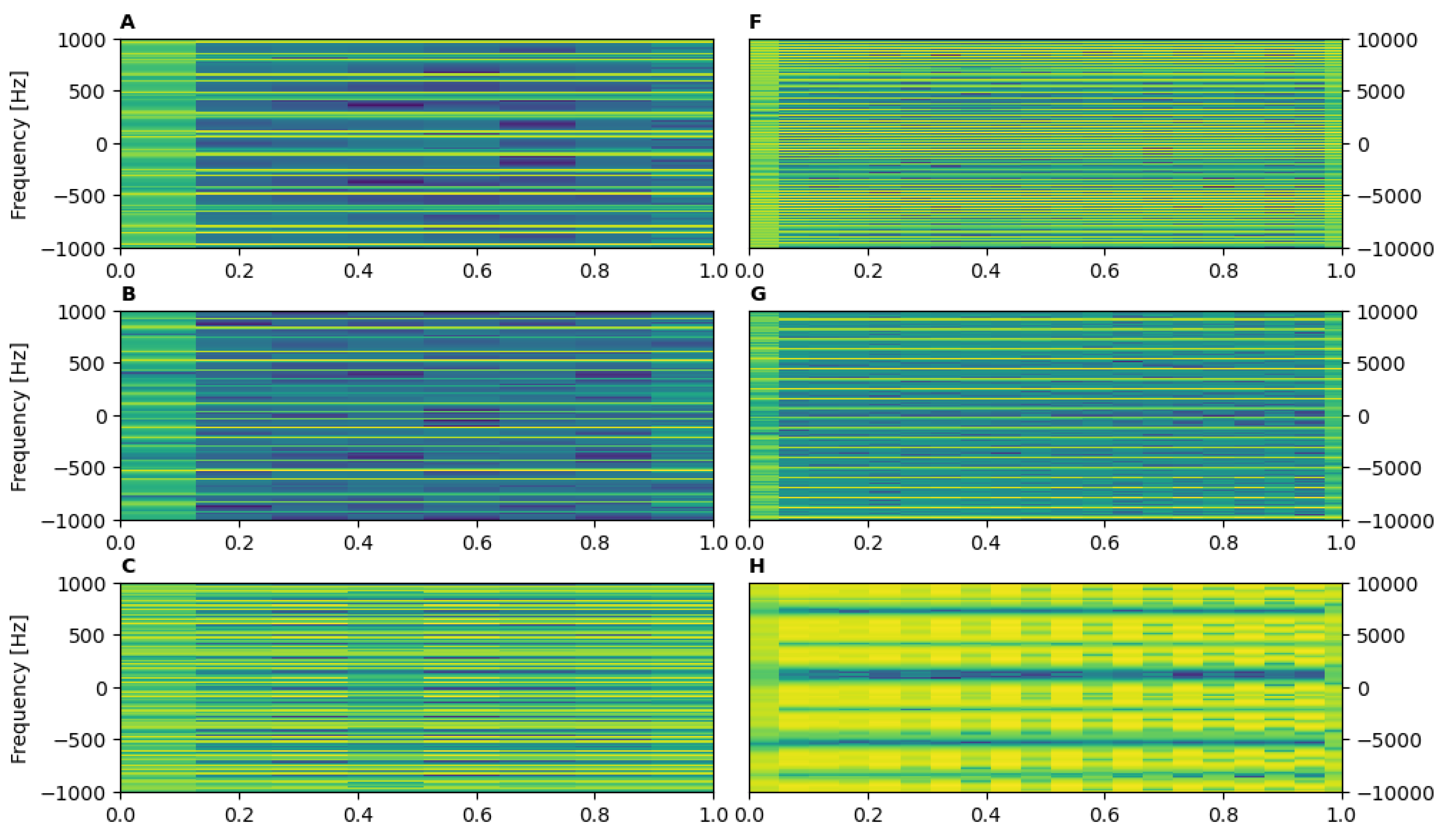
Figure 1 shows a long-window STFT spectrogram for each of the five drones outlined in Table 5. The signals were produced using radar parameters with the X-band (left column) and W-band (right column). For demonstration purposes, these signals have no augmentation. Notice the unique HERM line signature, or bands, within each spectrogram. These signatures are not an exact representation of the drones, but the important fact is that they are distinct from one another—just as we would expect in practice. Furthermore, these spectrograms would be easily identifiable by a convolutional network. We will investigate whether this remains true for signals that have undergone the previously discussed augmentation.

Before continuing with the creation of our neural network, it is prudent to examine whether the radar simulation is suitable for our purposes. To validate the Martin and Mulgrew model, we used the results of a laboratory experiment involving a commercial Typhoon H hexacopter drone. An X-band radar measured the drone, which was fixed in place and operating at a constant blade rotation frequency. Figure 2 shows the reflected radar signal and its corresponding long-window STFT spectrogram. This measured time-series is periodic, just like the simulated signals produced using Equation (2). Additionally, there appear to be HERM line signatures in the STFT, verifying the reasonability of the artificial data spectrograms shown previously. The spectrogram is not as clean as those seen in Figure 1 owing to background noise in the collected signal. This fact is addressed by our augmentation methods which make the simulated signals more realistic. Further validation would have been performed; however, the authors were limited by data access. From this point on, the Martin and Mulgrew model was pursued because it can capture many of the physical drone-blade parameters that contribute to the micro-Doppler signature.

2.4. Machine Learning Pipeline

Datasets were produced using the described data generation and augmentation methodology. A new dataset was created for each combination of radar specification and SNR, where the SNR ranged between 0 dB and 20 dB, in increments of 5 dB. The range for the SNR was motivated by the expected SNR of actual signals collected by our available radars. It is not easy to collect large real-drone datasets of high fidelity in practice. Thus, each dataset contained only 1000 spectrogram-training samples, equally-weighted among the six classes (five drones and noise). A smaller validation set of 350 samples was created to follow an approximate 60-20-20 percentage split. However, having the ability to produce the artificial data with relative ease, three test datasets—each with 350 samples—were uniquely generated. Therefore, when models were evaluated, the results contained standard deviation measures.

The architecture of the neural network has a convolutional and a linear portion. Given an input batch of spectrograms, they undergo three layers of convolution, SoftPlus activation, instance normalization, dropout, and periodic max pooling. The batch then undergoes linearization and passes through three hidden layers with ReLU activation. Finally, the loss is computed using the logits and cross-entropy. Figure 3 demonstrates this pipeline, with the dashed outline representing the model itself.

Recall that the two simulated radars used different PRF values, resulting in the size of the input spectrograms being different. A PRF of 20 kHz produces more data points per $0.3$ s in the signal, resulting in a larger spectrogram than a PRF of 2 kHz. The spectrogram sizes are $512\times 4$ and $2048\times 7$ for the 2 kHz PRF and 20 kHz PRF, respectively. This required the creation of two (similar) networks, one for each radar. The general architecture still holds because both networks differ only in kernel sizes and the number of hidden units in the linear layers.

A CNN model was trained for each training dataset (each dataset represents a unique radar and SNR combination). The training was conducted for 300 epochs, and the most generalizable models were selected through consideration of the training and validation loss and accuracy. All training occurred using PyTorch, a Python machine learning library, on an RTX 2060S GPU.

From the work of El Kafrawy et al. [37], the macro-${\mathrm{F}}_1$ score, referred to as the ${\mathrm{F}}_1$ score, was used to evaluate the performance of the trained models against the three test datasets. In many cases, the ${\mathrm{F}}_1$ score can be similar to pure accuracy. However, it benefits from considering false positives and false negatives through precision and recall, respectively, making it a preferred metric to accuracy. The formulation is provided in Equation (9), where C represents the number of classes (six), ${\mathrm{P}}_c$ is the precision and ${\mathrm{R}}_c$ is the recall, both of class $c\in \{1,2,\cdots ,C\}$ [37]. In their definitions, ${\mathrm{TP}}_c$, ${\mathrm{FP}}_c$, and ${\mathrm{FN}}_c$ are the number of true positives, false positives, and false negatives for class c, respectively.

$${\mathrm{F}}_1=\frac{2}{C}\sum _{c=1}^C\frac{{\mathrm{P}}_c{\mathrm{R}}_c}{{\mathrm{P}}_c+{\mathrm{R}}_c}$$

(9)

where

$$\begin{array}{cc}\hfill {\mathrm{P}}_c& =\frac{{\mathrm{TP}}_c}{{\mathrm{TP}}_c+{\mathrm{FP}}_c}\hfill \end{array}$$

(10)

$$\begin{array}{cc}\hfill {\mathrm{R}}_c& =\frac{{\mathrm{TP}}_c}{{\mathrm{TP}}_c+{\mathrm{FN}}_c}\hfill \end{array}$$

(11)

3. Results

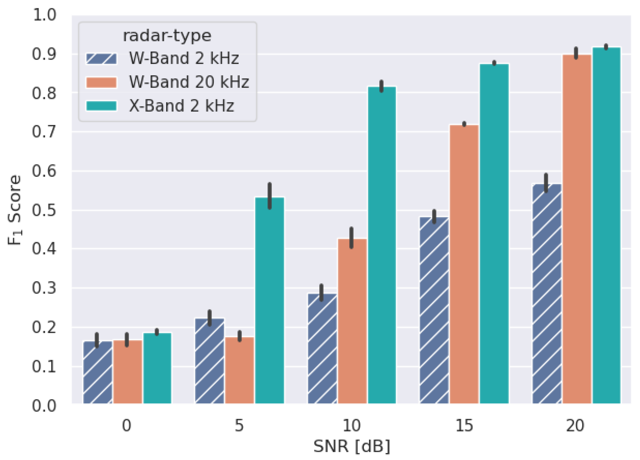
Presented in Figure 4 are the ${\mathrm{F}}_1$ score results of the trained models. The model for the X-band 2 kHz PRF radar achieved an ${\mathrm{F}}_1$ score of $0.816\pm 0.011$ at an SNR of 10 dB. The W-band 20 kHz PRF radar performed much worse, only reaching comparable results at 20 dB SNR. A W-band radar with a 2 kHz PRF was trained as a control model, which demonstrated weaker performance against the X-band radar at the same PRF. The X-band 2 kHz PRF radar, trained on 10 dB SNR, was used for further investigation moving forward due to its ability to perform relatively well under high noise conditions.

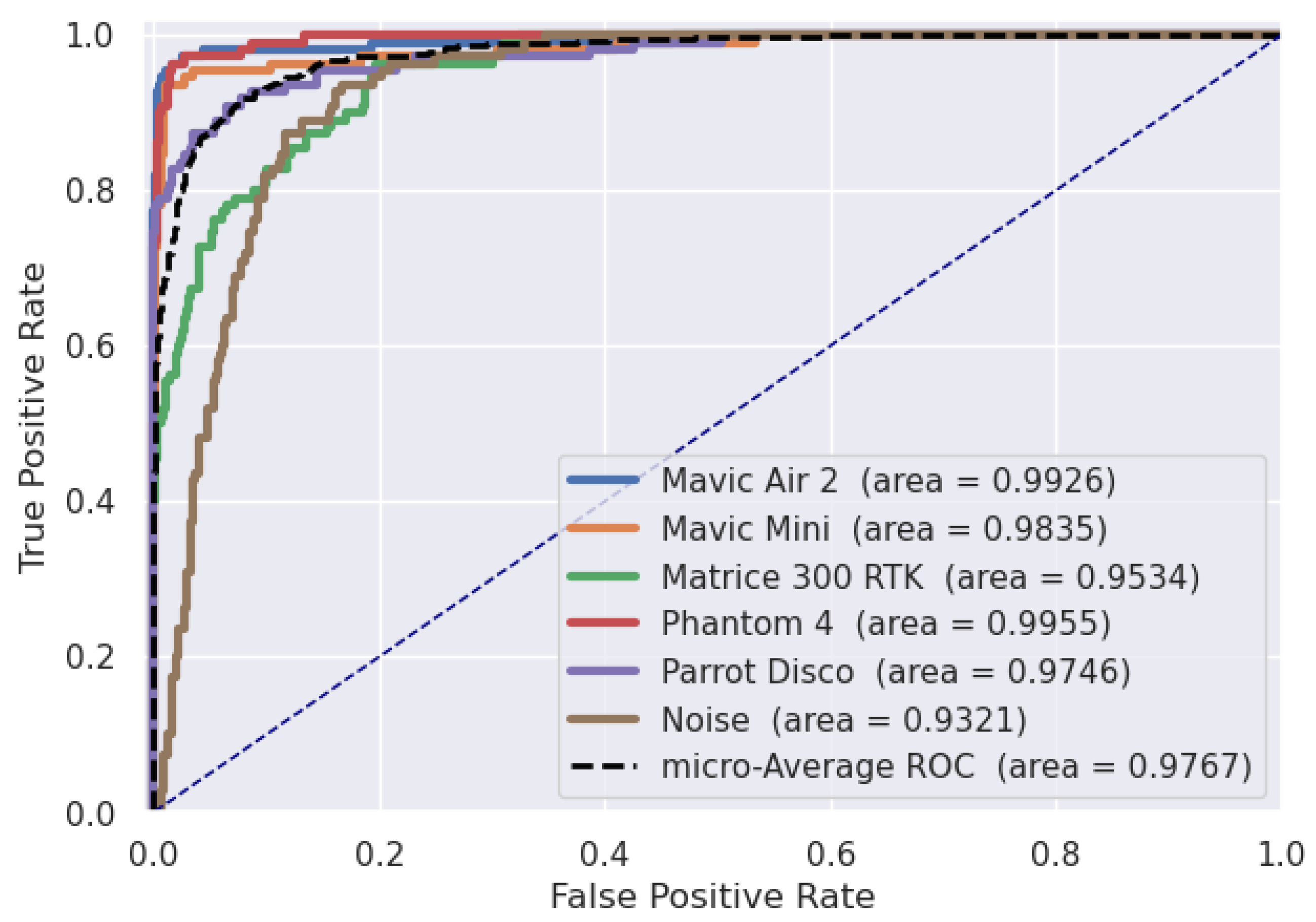
A multi-class confusion matrix and Receiver Operating Characteristic (ROC) curve were used to gain insight into the performance of the selected X-band model for each class. The selected model performs well at classifying drone classes. However, the classifier demonstrates a high false-negative rate when a false alarm sample (noise) is presented. As seen in Figure 5, noise is most often confused with the Matrice 300 RTK. Similarly, within Figure 6, noise has the lowest area under the ROC curve. Nevertheless, the model maintains a high average ROC area of 0.9767, suggesting a minimal compromise between true positives and false negatives.

Next, the robustness of the model against blade pitch and varying SNR values was investigated. The inclusion of blade pitch was a driving factor in using the more complex version of the Martin and Mulgrew equations to produce the artificial dataset. The results of the trained X-band 2 kHz PRF model against the blade pitch, ${\varphi }_p$, are in Figure 7. The model’s ${\mathrm{F}}_1$ score for the bins between 0 and $\pi /4$ remains close to the mean of 0.816 as expected. More importantly, the model remained robust, maintaining comparable performance when tested with ${\varphi }_p$ values outside those used in training.

In Figure 8, a similar analysis was conducted to determine the model’s robustness to varying SNR values. The model performs worse when tested on data with an SNR lower than 10 dB. In contrast, the same model can classify much more effectively as the SNR of the provided test data increases.

4. Discussion

Following the processes outlined in Section 2.3, artificial datasets were generated using the Martin and Mulgrew model, and CNN classifiers were trained for each dataset. Training each of these models enables us to quickly identify the required SNR of the data for drone classification and compare the performance of different radars for this application. Of particular importance, only 1000 spectrograms were present in each training set. This small size reflects the case where real drone data is minimal in applications. Obtained from the work of El Kafrawy et al., and presented in Equation (9), the multi-class ${\mathrm{F}}_1$ score metric was used to measure the performance of each trained model [37].

As found in Figure 4, the performance in the X-band is superior to that of the W-band for the chosen CNN. This is somewhat surprising as the W-band corresponds to a shorter wavelength and would intuitively result in better classification performance. There could be several reasons for this. Firstly, the 20 kHz PRF spectrogram is quite dense and holds a lot more information than a 2 kHz PRF STFT in the X-band. The additional complexity and detail may not be as robust against noise. By simulating a W-band radar at the same PRF as the X-band, we identify the reason for the discrepancy in performance lies in the transmitted wavelength parameter in the simulation. Note that we do not claim the X-band frequency is the best, but rather that it is better than W-band radars for typical parameters. Furthermore, X-band radars offer superior all-weather capabilities over other frequency bands. The W- and X- band radars were chosen for this paper because they are lighter and more portable than other band radars; however, it is possible that lower frequency bands (e.g., S-band and L-band) may provide superior performance over the X-band. This is undoubtedly a topic of exploration in future work. Additionally, our conclusion is limited to the choice of the model. A deeper CNN might yield a different conclusion, and it is something we plan to explore in future work.

In any case, the result is interesting and valuable. It suggests that an X-band radar with a PRF on the order of a few kHz can be highly effective in classifying drones under our simulation model. The lower PRF requirement in the X-band is also welcome as this leads to a longer unambiguous range. The 2 kHz PRF X-band classifier, trained on 10 dB SNR data, was selected for further investigation.

A multi-class confusion matrix and ROC curve were produced in Figure 5 and Figure 6, respectively, which revealed shortcomings in the selected model. The noise class exhibits the weakest performance in both, and the confusion matrix reveals that noise is most often misclassified as a DJI Matrice 300 RTK drone. The reasoning for this misclassification is not immediately apparent. However, a qualitative consideration of Figure 1 suggests that spectrograms with a dense micro-Doppler signature (HERM lines) might be more easily confused with noise. The Matrice 300 RTK, in particular, has a very dense signature. On the other hand, an STFT of Gaussian noise contains no distinct signature or obvious spatial information. Under the low, 10 dB SNR conditions, the Matrice 300 RTK spectrogram likely becomes augmented to the point where it begins to resemble the random-looking noise STFTs. This result emphasizes the need for reliable drone detection models and algorithms, as false alarms can easily be confused with some drone types during the classification process.

Consideration of Figure 7 shows that model performance is invariant to different values of $\varphi$, even for values not included in the training dataset. This result is important because it suggests that classification performance is mostly unaffected by the pitch of the drone blades. In a similar analysis against varying SNR, the trained model demonstrated a linear trend in performance. The model performed worse when evaluated using data with an SNR lower than the 10 dB used for training while showing superior performance on less noisy, higher dB data samples. This result is shown in Figure 8. Both of these results inform that when training drone classifiers, the blade pitch of the samples is not critical. Additionally, models should maintain linear performance near the SNR of the training samples.

In Figure 4, Figure 7 and Figure 8 we observe the standard deviation of the test results shown by vertical lines. These were produced by evaluating the model’s performance on three different test sets. The small size of the standard deviations strengthens our results’ confidence and, therefore, the efficacy of our CNN classifier.

5. Conclusions

This paper investigated the feasibility of classifying drones using radar signals and machine learning. The utilized datasets were generated using the Martin and Mulgrew model with realistic drone parameters. Five distinct drones were classified, and a sixth noise (false alarm) class was also considered during our analysis. We show that it is possible to train a CNN model to classify drones in low SNR scenarios, using a signal of just 0.3 s in duration. We find that practically realizable radars (e.g., X-band with 2 kHz PRF) can lead to a ${\mathrm{F}}_1$ performance of $0.816\pm 0.011$ using training data of 10 dB SNR. Further analysis of the trained model shows that it remains robust to varying drone blade pitch and linearly decreases and increases in performance with the SNR of the signal. However, the model becomes less viable when false alarms are presented, as they can be confused with some drone classes. We wish to stress that the presented analysis is based on a simple model and should be corroborated with higher-fidelity models.

Our goals are to continue exploring the Martin and Mulgrew model for the purpose of constructing drone classifiers. Specifically, we wish to investigate the effect of transmitted wavelengths on model performance. An in-depth comparison of the classification results using a more comprehensive range of radars is a good topic for future work. Further exploration should uncover why the W-band radar signals provided worse data than the X-band for use in our CNN. As stated previously, the Martin and Mulgrew model assumes that the modelled drone has a single rotor; however, many real drones have up to eight rotors. Future work could investigate an adapted Martin and Mulgrew model proposed in [35] which considers multiple rotors. Moreover, it would be interesting to compare the performance of models trained using samples of shorter duration but with higher PRF against training samples of longer duration with lower PRF values. Consideration of different machine learning approaches and more complex CNN architectures will also be of interest. In parallel, recognizing that simulations produce results under controlled and ideal conditions, we wish to elucidate the applicability of the trained CNN models on real drone data. This can be investigated via a direct application of the model on real data or through a transfer learning process where the trained models are used as a starting point for further training.