
Prototype Development of Cross-Shaped Microphone Array System for Drone Localization Based on Delay-and-Sum Beamforming in GNSS-Denied Areas

 , , and
Abstract
:1. Introduction
2. Related Work
- Our proposed method can detect the horizontal position of a drone using three parameters obtained from the drone and our cross-shaped microphone array system. The challenging detection range is greater than the previous approach [42].
- To the best of our knowledge, this is the first study to demonstrate and evaluate drone localization based on DAS beamforming used in GNSS-denied areas.
3. Proposed Method
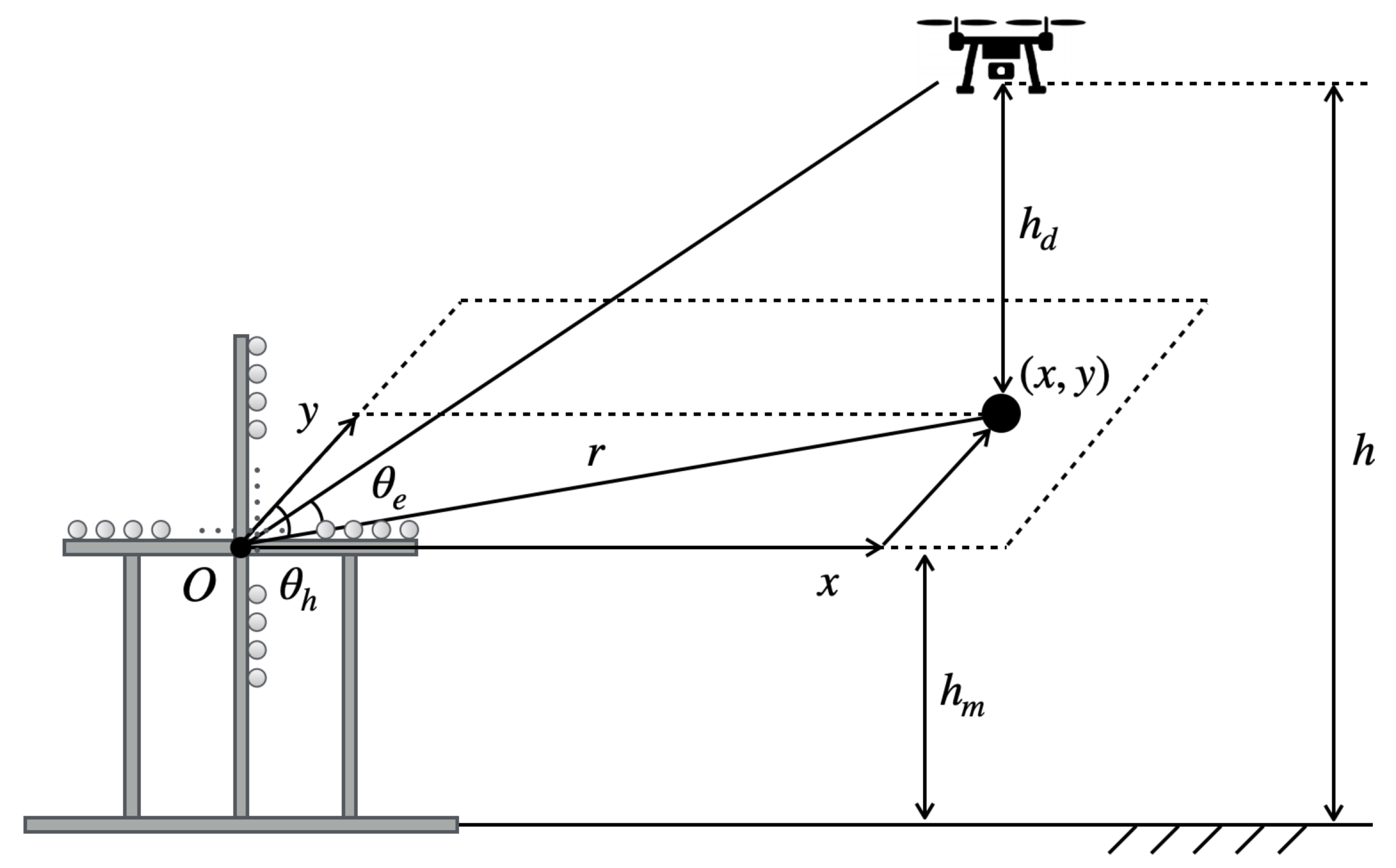
3.1. Acoustic Localization Method
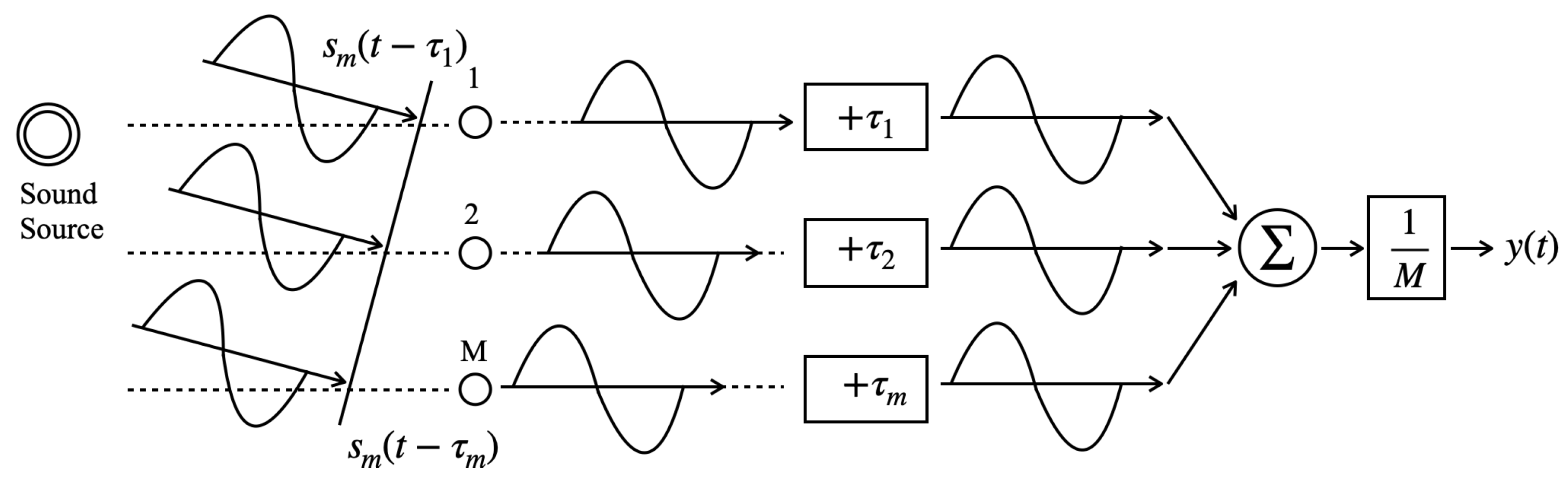
3.2. Delay-and-Sum Beamforming
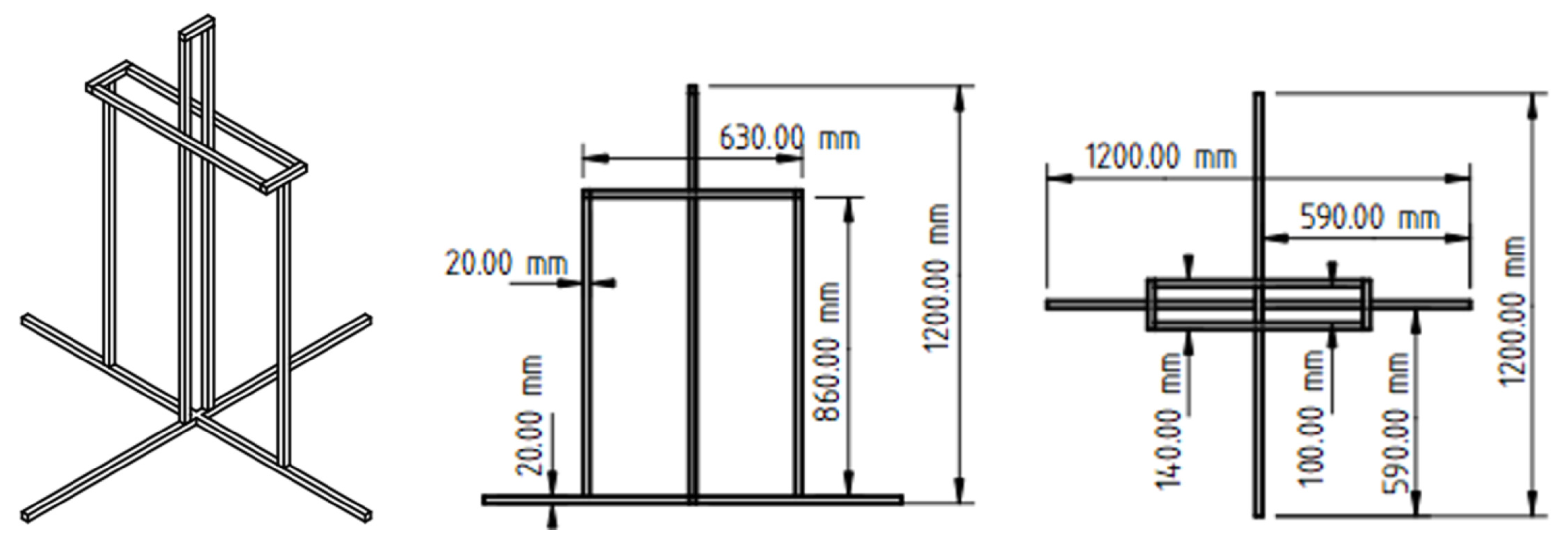
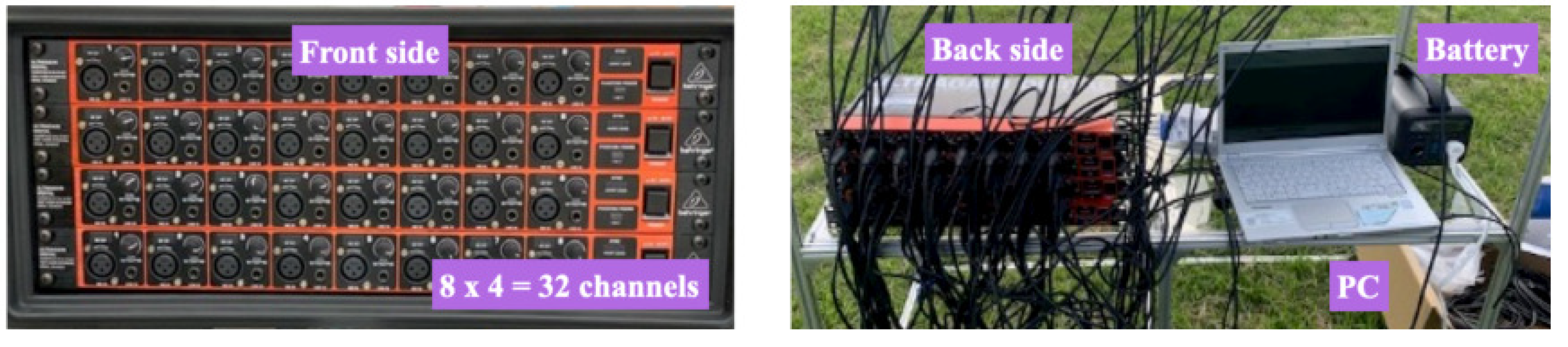
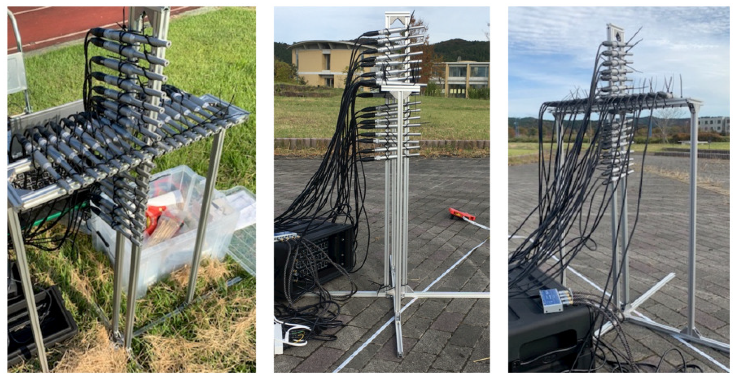
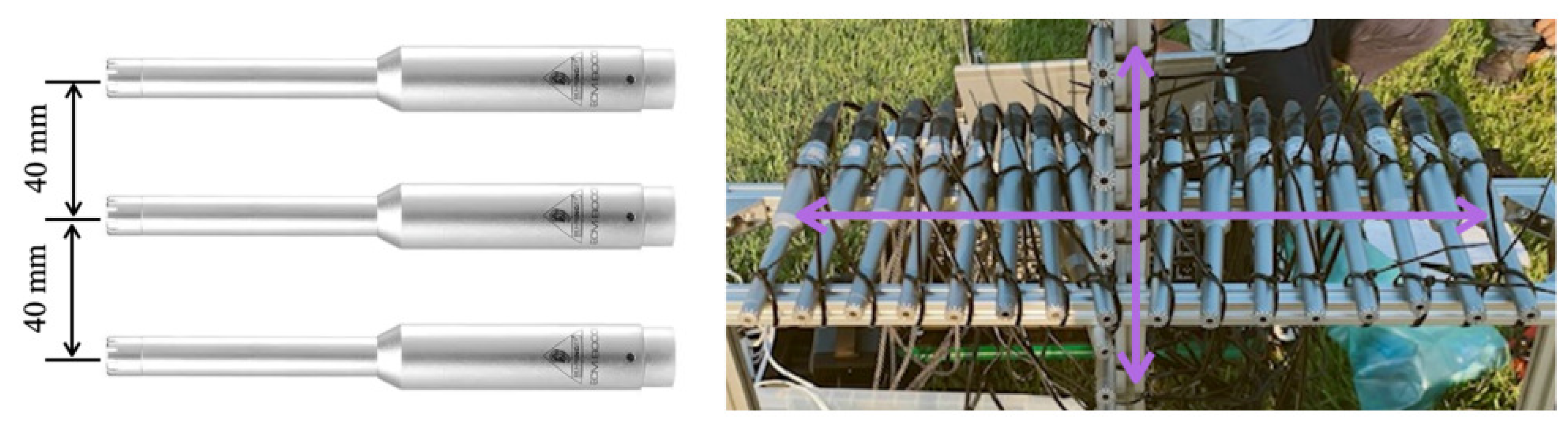
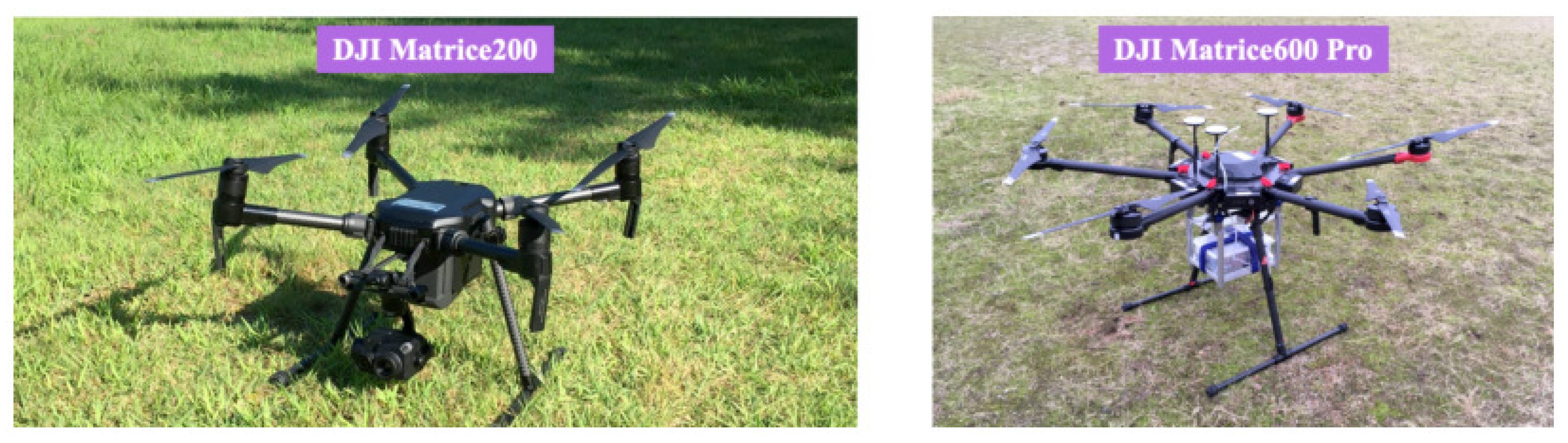
3.3. Devices for Experimentation
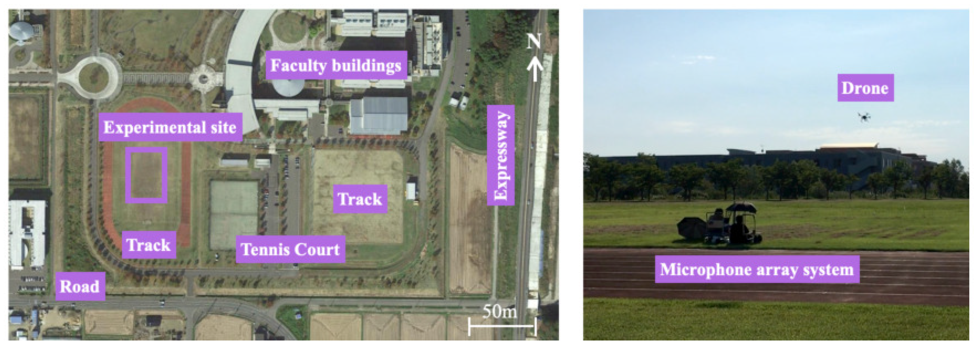
4. Position Estimation Experiment
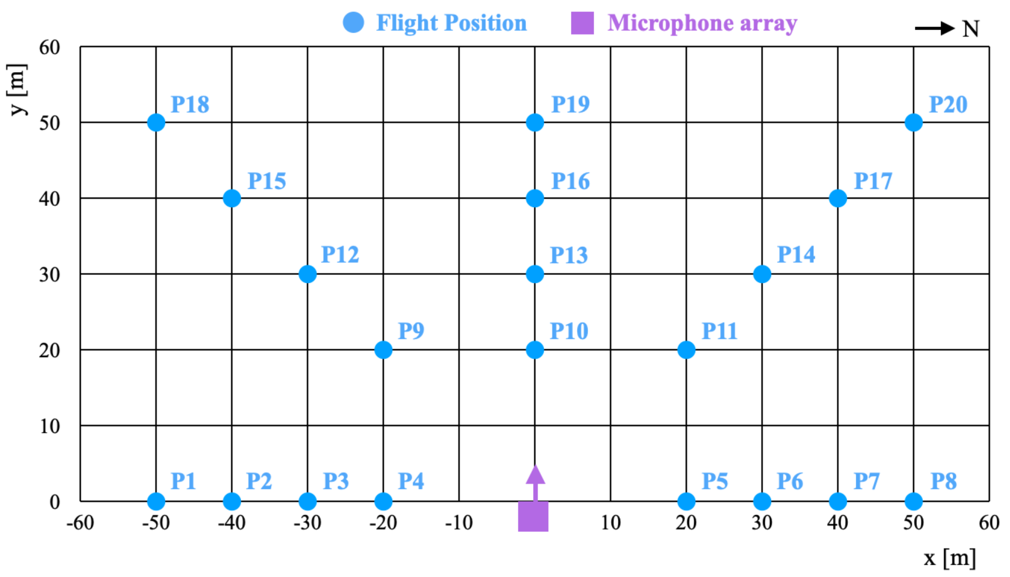
4.1. Benchmark Datasets
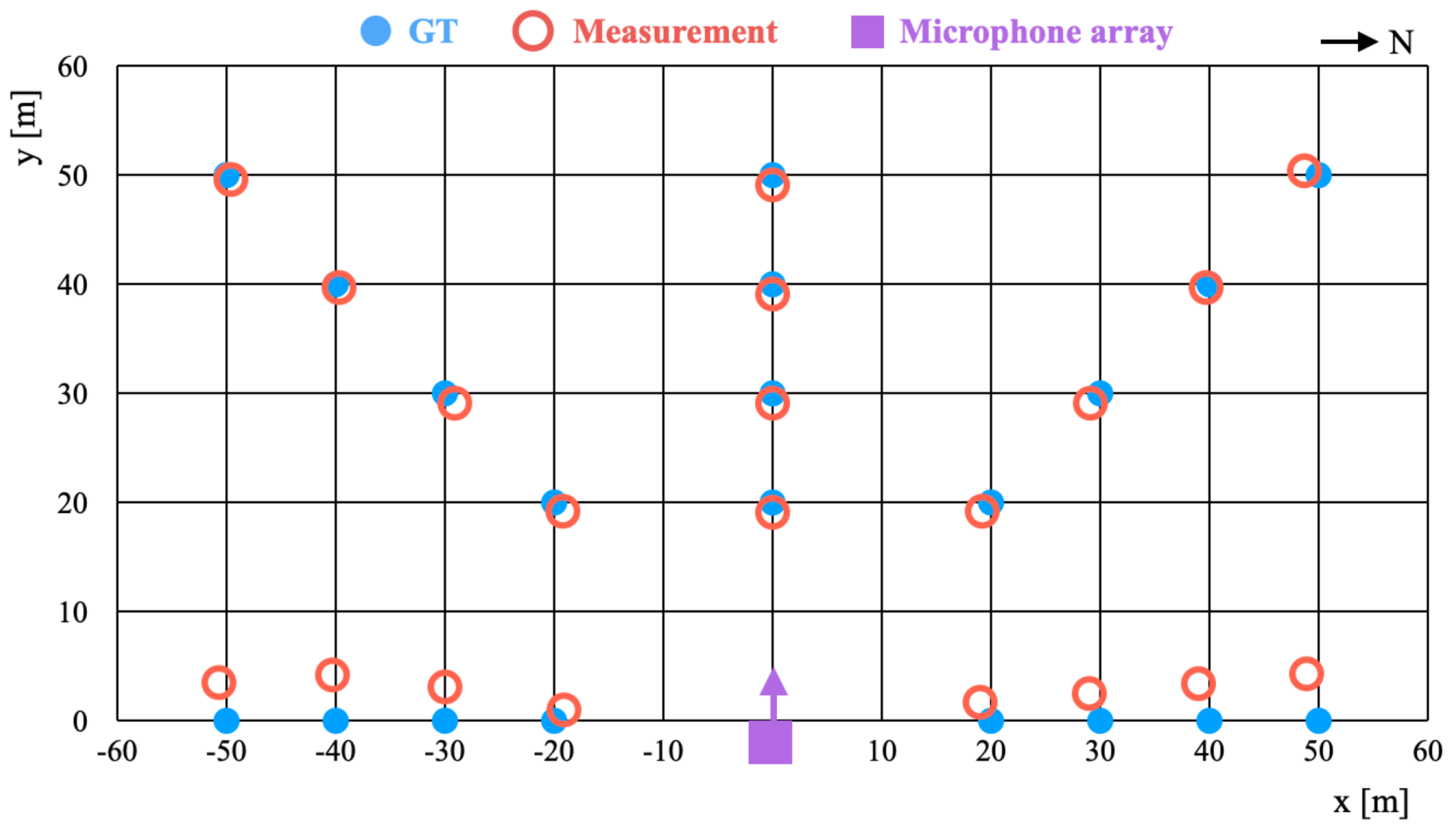
- A 2D position on the ground was measured using a tape measure and marked.
- After placing a drone at the mark, it was flown to an arbitrary height in the vertical direction.
- The 3D flight position was confirmed by visual observation from the ground and field-of-view (FOV) images transmitted from an onboard camera of the drone.
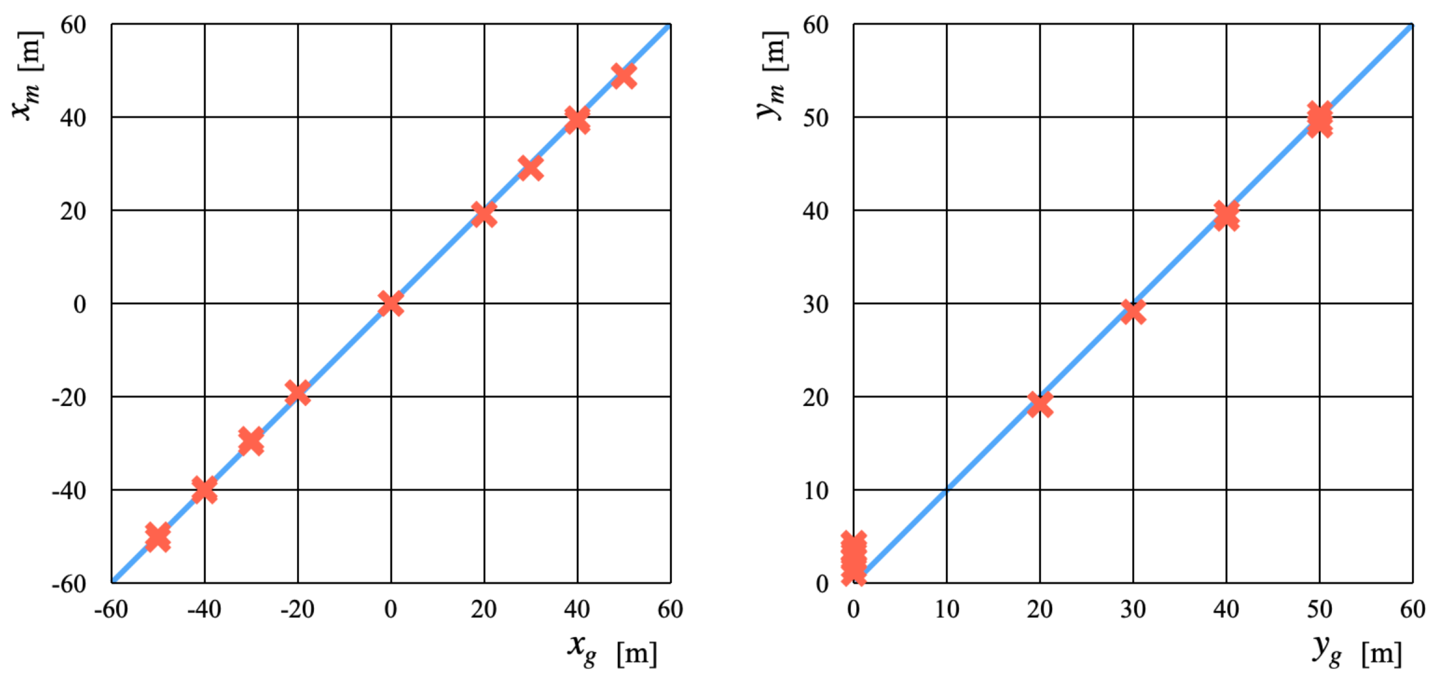
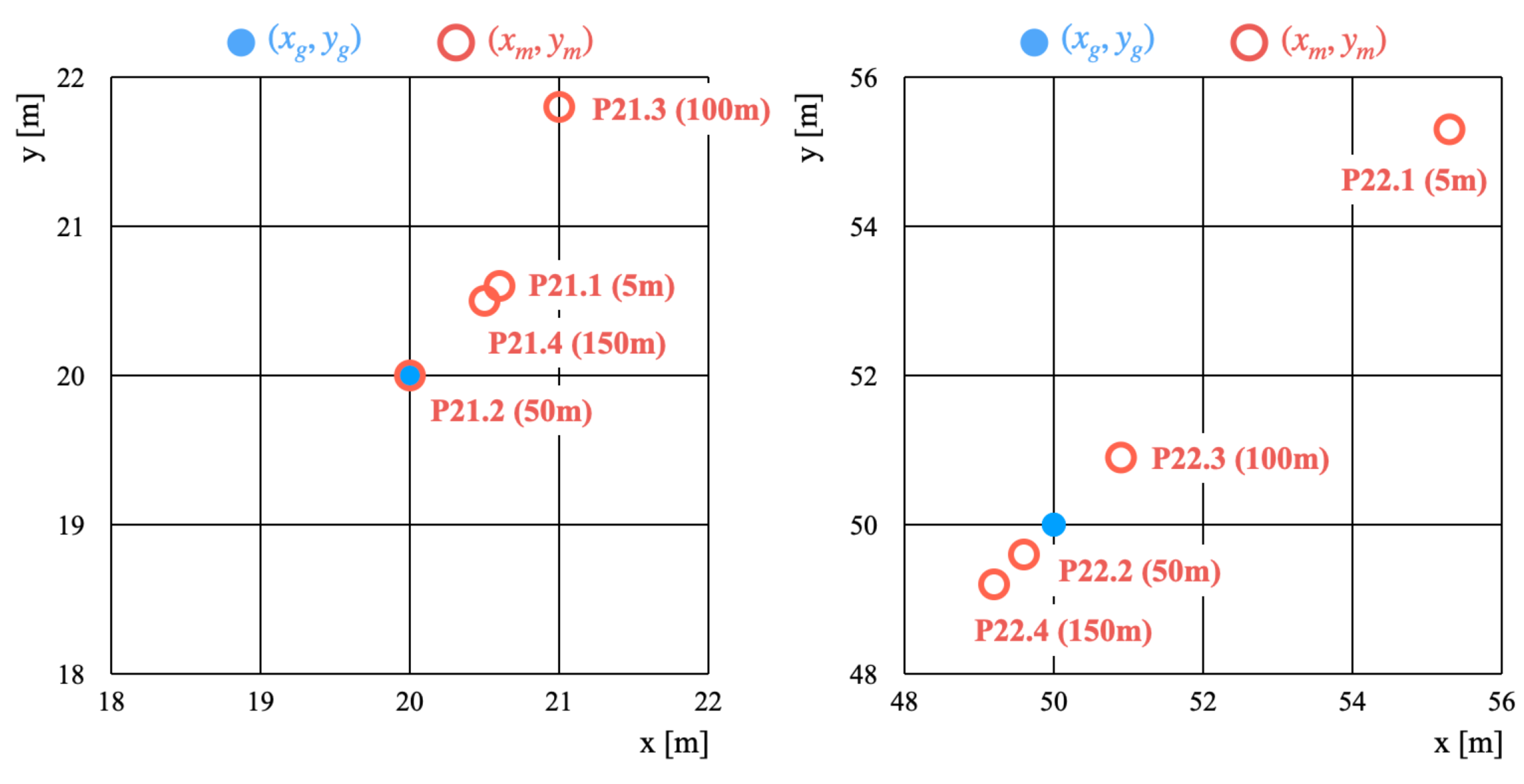
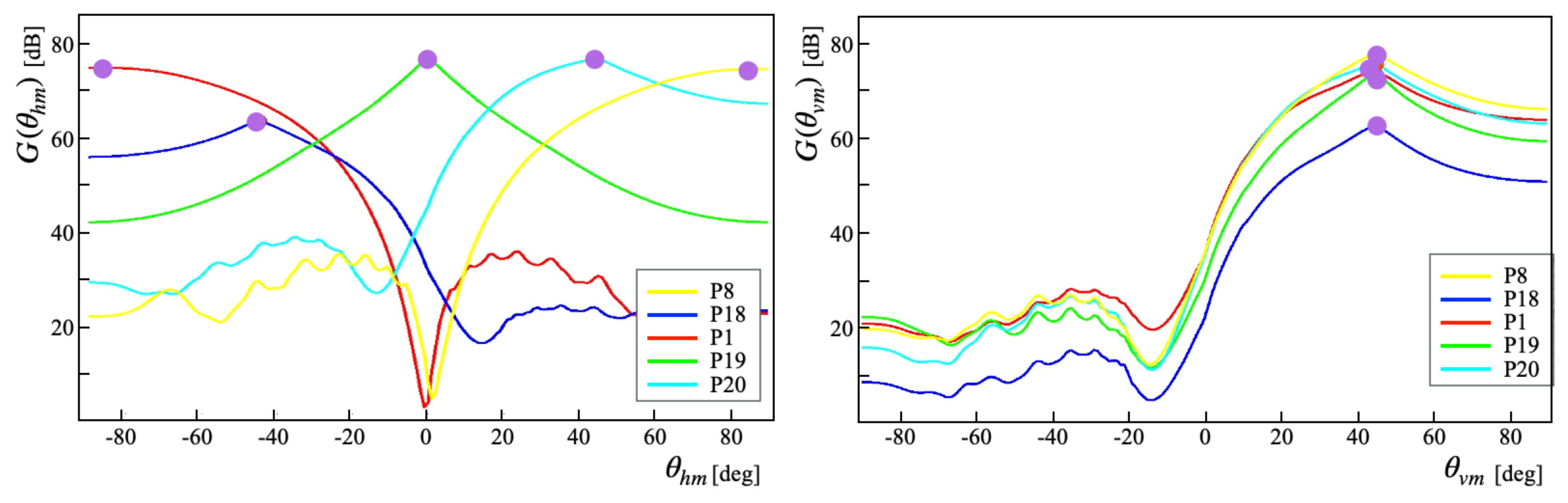
4.2. Experiment Results
4.3. Discussion
5. Conclusions
Author Contributions
Funding
Institutional Review Board Statement
Informed Consent Statement
Data Availability Statement
Acknowledgments
Conflicts of Interest
Abbreviations
| A/D | analog-to-digital |
| BDS | BeiDou navigation satellite system |
| CoNN | concurrent neural network |
| DAS | delay-and-sum |
| FOV | field of view |
| GCC-PHAT | cross-correlation phase transform |
| GLONASS | global navigation satellite system |
| GNSS | global navigation satellite systems |
| GPS | global positioning system |
| GT | ground truth |
| LiDAR | light detection and ranging |
| RF | radio-frequency |
| RTK | real-time kinematic |
| SRP-PHAT | steered-response phase transform |
| SNR | signal-to-noise ratio |
| SLAM | simultaneous localization and mapping |
| TDOA | time difference of arrival |
| UAV | unmanned aerial vehicle |
| YOLO | you only look once |
References
- Floreano, D.; Wood, R. Technology and the Future of Small Autonomous Drones. Nature 2015, 521, 460–466. [Google Scholar] [CrossRef] [PubMed] [Green Version]
- Henkel, P.; Sperl, A. Real-Time Kinematic Positioning for Unmanned Air Vehicles. In Proceedings of the IEEE Aerospace Conference, Big Sky, MT, USA, 5–12 March 2016; pp. 1–7. [Google Scholar]
- Rao, U.M.; Deepak, V. Review on Application of Drone Systems in Precision Agriculture. Procedia Comput. Sci. 2018, 133, 502–509. [Google Scholar]
- Bacco, M.; Berton, A.; Ferro, E.; Gennaro, C.; Gotta, A.; Matteoli, S.; Paonessa, F.; Ruggeri, M.; Virone, G.; Zanella, A. Smart Farming: Opportunities, Challenges and Technology Enablers. In Proceedings of the IoT Vertical and Topical Summit on Agriculture, Tuscany, Italy, 8–9 May 2018; pp. 1–6. [Google Scholar]
- Shakhatreh, H.; Sawalmeh, A.H.; Fuqaha, A.A.; Dou, Z.; Almaita, E.; Khalil, I.; Othman, N.S.; Khreishah, A.; Guizani, M. Unmanned Aerial Vehicles (UAVs): A Survey on Civil Applications and Key Research Challenges. IEEE Access 2019, 7, 48572–48634. [Google Scholar]
- Na, W.S.; Baek, J. Impedance-Based Non-Destructive Testing Method Combined with Unmanned Aerial Vehicle for Structural Health Monitoring of Civil Infrastructures. Appl. Sci. 2017, 7, 15. [Google Scholar] [CrossRef] [Green Version]
- Madokoro, H.; Sato, K.; Shimoi, N. Vision-Based Indoor Scene Recognition from Time-Series Aerial Images Obtained Using a MAV Mounted Monocular Camera. Drones 2019, 3, 22. [Google Scholar] [CrossRef] [Green Version]
- Shahmoradi, J.; Talebi, E.; Roghanchi, P.; Hassanalian, M. A Comprehensive Review of Applications of Drone Technology in the Mining Industry. Drones 2020, 4, 34. [Google Scholar] [CrossRef]
- Li, Y.; Liu, C. Applications of Multirotor Drone Technologies in Construction Management. Int. J. Constr. Manag. 2019, 19, 401–412. [Google Scholar] [CrossRef]
- Kellermann, R.; Biehle, T.; Fischer, L. Drones for parcel and passenger transportation: A literature review of Transportation Research. Interdiscip. Perspect. 2020, 4, 100088. [Google Scholar]
- He, D.; Chan, S.; Guizani, M. Drone-Assisted Public Safety Networks: The Security Aspect. IEEE Commun. Mag. 2017, 55, 218–223. [Google Scholar] [CrossRef]
- Alotaibi, E.T.; Alqefari, S.S.; Koubaa, A. LSAR: Multi-UAV Collaboration for Search and Rescue Missions. IEEE Access 2019, 7, 55817–55832. [Google Scholar] [CrossRef]
- Shen, N.; Chen, L.; Liu, J.; Wang, L.; Tao, T.; Wu, D.; Chen, R. A Review of Global Navigation Satellite System (GNSS)-Based Dynamic Monitoring Technologies for Structural Health Monitoring. Remote Sens. 2019, 11, 1001. [Google Scholar] [CrossRef] [Green Version]
- Chen, C.; Tian, Y.; Lin, L.; Chen, S.; Li, H.; Wang, Y.; Su, K. Obtaining World Coordinate Information of UAV in GNSS Denied Environments. Sensors 2020, 20, 2241. [Google Scholar]
- Taha, B.; Shoufan, A. Machine Learning-Based Drone Detection and Classification: State-of-the-Art in Research. IEEE Access 2019, 7, 138669–138682. [Google Scholar] [CrossRef]
- Lykou, G.; Moustakas, D.; Gritzalis, D. Defending Airports from UAS: A Survey on Cyber-Attacks and Counter-Drone Sensing Technologies. Sensors 2020, 20, 3537. [Google Scholar] [CrossRef] [PubMed]
- Park, S.; Kim, H.T.; Lee, S.; Joo, H.; Kim, H. Survey on Anti-Drone Systems: Components, Designs, and Challenges. IEEE Access 2021, 9, 42635–42659. [Google Scholar] [CrossRef]
- Leonard, J.J.; Durrant-Whyte, H.F. Simultaneous Map Building and Localization for an Autonomous Mobile Robot. In Proceedings of the IEEE/RSJ International Workshop on Intelligent Robots and Systems, Osaka, Japan, 3–5 November 1991; pp. 1442–1447. [Google Scholar]
- Perez-Grau, F.J.; Ragel, R.; Caballero, F.; Viguria, A.; Ollero, A. An architecture for robust UAV navigation in GPS-denied areas. J. Field Robot. 2018, 35, 121–145. [Google Scholar] [CrossRef]
- López, E.; García, S.; Barea, R.; Bergasa, L.M.; Molinos, E.J.; Arroyo, R.; Romera, E.; Pardo, S.A. Multi-Sensorial Simultaneous Localization and Mapping (SLAM) System for Low-Cost Micro Aerial Vehicles in GPS-Denied Environments. Sensors 2017, 17, 802. [Google Scholar] [CrossRef]
- Krul, S.; Pantos, C.; Frangulea, M.; Valente, J. Visual SLAM for Indoor Livestock and Farming Using a Small Drone with a Monocular Camera: A Feasibility Study. Drones 2021, 5, 41. [Google Scholar] [CrossRef]
- Bloesch, M.; Czarnowski, J.; Clark, R.; Leutenegger, S.; Davison, A.J. CodeSLAM–Learning a Compact, Optimisable Representation for Dense Visual SLAM. In Proceedings of the IEEE/CVF Conference on Computer Vision and Pattern Recognition, Salt Lake City, UT, USA, 18–23 June 2018; pp. 2560–2568. [Google Scholar]
- Motlagh, H.D.K.; Lotfi, F.; Taghirad, H.D.; Germi, S.B. Position Estimation for Drones based on Visual SLAM and IMU in GPS-denied Environment. In Proceedings of the 7th International Conference on Robotics and Mechatronics, Tehran, Iran, 20–21 November 2019; pp. 120–124. [Google Scholar]
- Karimi, M.; Oelsch, M.; Stengel, O.; Babaians, E.; Steinbach, E. LoLa-SLAM: Low-Latency LiDAR SLAM Using Continuous Scan Slicing. IEEE Robot. Autom. Lett. 2021, 6, 2248–2255. [Google Scholar] [CrossRef]
- Horaud, R.; Hansard, M.; Evangelidis, G.; Ménier, C. An overview of depth cameras and range scanners based on time-of-flight technologies. Mach. Vis. Appl. 2016, 27, 1005–1020. [Google Scholar] [CrossRef] [Green Version]
- Taketomi, T.; Uchiyama, H.; Ikeda, S. Visual SLAM algorithms: A survey from 2010 to 2016. IPSJ Trans. Comput. Vis. Appl. 2017, 9, 16. [Google Scholar] [CrossRef]
- Tribelhorn, B.; Dodds, Z. Evaluating the Roomba: A low-cost, ubiquitous platform for robotics research and education. In Proceedings of the IEEE International Conference on Robotics and Automation, Rome, Italy, 10–14 April 2007; pp. 1393–1399. [Google Scholar]
- Mashood, A.; Dirir, A.; Hussein, M.; Noura, H.; Awwad, F. Quadrotor Object Tracking Using Real-Time Motion Sensing. In Proceedings of the 5th International Conference on Electronic Devices, Systems and Applications, Ras Al Khaimah, United Arab Emirates, 6–8 December 2016; pp. 1–4. [Google Scholar]
- LeCun, Y.; Bengio, Y.; Hinton, G. Deep Learning. Nature 2015, 521, 436–444. [Google Scholar] [PubMed]
- Nijim, M.; Mantrawadi, N. Drone Classification and Identification System by Phenome Analysis Using Data Mining Techniques. In Proceedings of the IEEE Symposium on Technologies for Homeland Security, Waltham, MA, USA, 10–11 May 2016; pp. 1–5. [Google Scholar]
- Jeon, S.; Shin, J.W.; Lee, Y.J.; Kim, W.H.; Kwon, Y.; Yang, H.Y. Empirical Study of Drone Sound Detection in Real-Life Environment with Deep Neural Networks. In Proceedings of the 25th European Signal Processing Conference, Kos, Greece, 28 August–2 September 2017; pp. 1858–1862. [Google Scholar]
- Bernardini, A.; Mangiatordi, F.; Pallotti, E.; Capodiferro, L. Drone detection by acoustic signature identification. Electron. Imaging 2017, 10, 60–64. [Google Scholar] [CrossRef]
- Kim, J.; Park, C.; Ahn, J.; Ko, Y.; Park, J.; Gallagher, J.C. Real-Time UAV Sound Detection and Analysis System. In Proceedings of the IEEE Sensors Applications Symposium, Glassboro, NJ, USA, 13–15 March 2017; pp. 1–5. [Google Scholar]
- Yue, X.; Liu, Y.; Wang, J.; Song, H.; Cao, H. Software Defined Radio and Wireless Acoustic Networking for Amateur Drone Surveillance. IEEE Commun. Mag. 2018, 56, 90–97. [Google Scholar] [CrossRef]
- Seo, Y.; Jang, B.; Im, S. Drone Detection Using Convolutional Neural Networks with Acoustic STFT Features. In Proceedings of the 15th IEEE International Conference on Advanced Video Signal Based Surveillance, Auckland, New Zealand, 27–30 November 2018; pp. 1–6. [Google Scholar]
- Matson, E.; Yang, B.; Smith, A.; Dietz, E.; Gallagher, J. UAV Detection System with Multiple Acoustic Nodes Using Machine Learning Models. In Proceedings of the third IEEE International Conference on Robotic Computing, Naples, Italy, 25–27 February 2019; pp. 493–498. [Google Scholar]
- Sedunov, A.; Haddad, D.; Salloum, H.; Sutin, A.; Sedunov, N.; Yakubovskiy, A. Stevens Drone Detection Acoustic System and Experiments in Acoustics UAV Tracking. In Proceedings of the IEEE International Symposium on Technologies for Homeland Security, Woburn, MA, USA, 5–6 November 2019; pp. 1–7. [Google Scholar]
- Cobos, M.; Marti, A.; Lopez, J.J. A Modified SRP-PHAT Functional for Robust Real-Time Sound Source Localization With Scalable Spatial Sampling. IEEE Signal Process. Lett. 2011, 18, 71–74. [Google Scholar] [CrossRef]
- Knapp, C.; Carter, G. The Generalized Correlation Method for Estimation of Time Delay. IEEE Trans. Acoust. Speech Signal Process. 1976, 24, 320–327. [Google Scholar] [CrossRef] [Green Version]
- Chang, X.; Yang, C.; Wu, J.; Shi, X.; Shi, Z. A Surveillance System for Drone Localization and Tracking Using Acoustic Arrays. In Proceedings of the IEEE 10th Sensor Array and Multichannel Signal Processing Workshop, Sheffield, UK, 8–11 July 2018; pp. 573–577. [Google Scholar]
- Dumitrescu, C.; Minea, M.; Costea, I.M.; Cosmin Chiva, I.; Semenescu, A. Development of an Acoustic System for UAV Detection. Sensors 2020, 20, 4870. [Google Scholar] [CrossRef]
- Blanchard, T.; Thomas, J.H.; Raoof, K. Acoustic Localization and Tracking of a Multi-Rotor Unmanned Aerial Vehicle Using an Array with Few Microphones. J. Acoust. Soc. Am. 2020, 148, 1456. [Google Scholar] [CrossRef] [PubMed]
- Zunino, A.; Crocco, M.; Martelli, S.; Trucco, A.; Bue, A.D.; Murino, V. Seeing the Sound: A New Multimodal Imaging Device for Computer Vision. In Proceedings of the IEEE International Conference on Computer Vision, Santiago, Chile, 13–16 December 2015; pp. 6–14. [Google Scholar]
- Liu, H.; Wei, Z.; Chen, Y.; Pan, J.; Lin, L.; Ren, Y. Drone Detection Based on an Audio-Assisted Camera Array. In Proceedings of the IEEE Third International Conference on Multimedia Big Data, Laguna Hills, CA, USA, 19–21 April 2017; pp. 402–406. [Google Scholar]
- Svanstr´’om, F.; Englund, C.; Alonso-Fernandez, F. Real-Time Drone Detection and Tracking with Visible, Thermal and Acoustic Sensors. In Proceedings of the 25th International Conference on Pattern Recognition, Milan, Italy, 10–15 January 2021; pp. 7265–7272. [Google Scholar]
- Redmon, J.; Farhadi, A. YOLO9000: Better, Faster, Stronger. In Proceedings of the IEEE Conference on Computer Vision and Pattern Recognition, Honolulu, HI, USA, 21–26 July 2017; pp. 7263–7271. [Google Scholar]
- Izquierdo, A.; del Val, L.; Villacorta, J.J.; Zhen, W.; Scherer, S.; Fang, Z. Feasibility of Discriminating UAV Propellers Noise from Distress Signals to Locate People in Enclosed Environments Using MEMS Microphone Arrays. Sensors 2020, 20, 597. [Google Scholar] [CrossRef] [Green Version]
- Van Veen, B.D.; Buckley, K.M. Beamforming: A Versatile Approach to Spatial Filtering. IEEE ASSP Mag. 1988, 5, 4–24. [Google Scholar] [CrossRef]
- Modsching, M.; Kramer, R.; ten Hagen, K. Field Trial on GPS Accuracy in a Medium Size City: The Influence of Built-up. In Proceedings of the Third Workshop on Positioning, Navigation and Communication, Hannover, Germany, 16 March 2006. [Google Scholar]


| Items | Matrice 200 | Matrice 600 Pro |
|---|---|---|
| Diagonal wheelbase | 643 mm | 1133 mm |
| Dimensions (L × W × H) | 887 × 880 × 378 mm | 1668 × 1518 × 727 mm |
| Rotor quantity | 4 | 6 |
| Weight (including standard batteries) | 6.2 kg | 9.5 kg |
| Payload | 2.3 kg | 6.0 kg |
| Maximum ascent speed | 5 m/s | |
| Maximum descent speed | 3 m/s | |
| Maximum wind resistance | 12 m/s | 8 m/s |
| Maximum flight altitude | 3000 m | 2500 m |
| Operating temperature | C to C | C to C |
| GNSS | GPS + GLONASS | |
| Position | Group | [m] | [m] | h [m] | [] | [] |
|---|---|---|---|---|---|---|
| P1 | 4 | −50 | 0 | 50 | −90 | 45 |
| P2 | 3 | −40 | 0 | 40 | −90 | 45 |
| P3 | 2 | −30 | 0 | 30 | −90 | 45 |
| P4 | 1 | −20 | 0 | 20 | −90 | 45 |
| P5 | 1 | 20 | 0 | 20 | 90 | 45 |
| P6 | 2 | 30 | 0 | 30 | 90 | 45 |
| P7 | 3 | 40 | 0 | 40 | 90 | 45 |
| P8 | 4 | 50 | 0 | 50 | 90 | 45 |
| P9 | 1 | −20 | 20 | 28 | −45 | 45 |
| P10 | 1 | 0 | 20 | 20 | 0 | 45 |
| P11 | 1 | 20 | 20 | 28 | 45 | 45 |
| P12 | 2 | −30 | 30 | 42 | −45 | 45 |
| P13 | 2 | 0 | 30 | 30 | 0 | 45 |
| P14 | 2 | 30 | 30 | 42 | 45 | 45 |
| P15 | 3 | −40 | 40 | 57 | −45 | 45 |
| P16 | 3 | 0 | 40 | 40 | 0 | 45 |
| P17 | 3 | 40 | 40 | 57 | 45 | 45 |
| P18 | 4 | −50 | 50 | 71 | −45 | 45 |
| P19 | 4 | 0 | 50 | 50 | 0 | 45 |
| P20 | 4 | 50 | 50 | 71 | 45 | 45 |
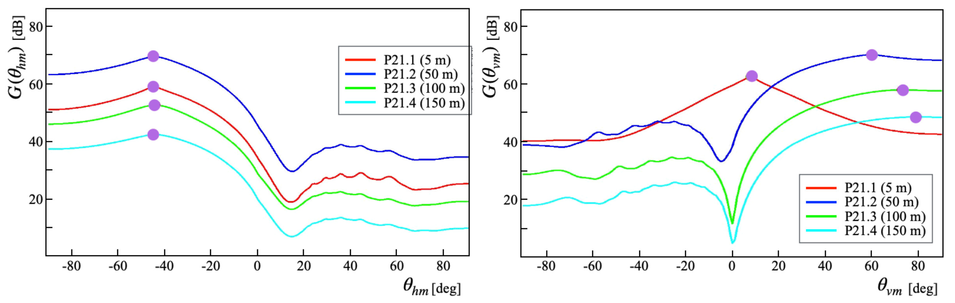
| P21.1 | – | 20 | 20 | 5 | 45 | 8 |
| P21.2 | – | 20 | 20 | 50 | 45 | 60 |
| P21.3 | – | 20 | 20 | 100 | 45 | 74 |
| P21.4 | – | 20 | 20 | 150 | 45 | 79 |
| P22.1 | – | 50 | 50 | 5 | 45 | 3 |
| P22.2 | – | 50 | 50 | 50 | 45 | 35 |
| P22.3 | – | 50 | 50 | 100 | 45 | 54 |
| P22.4 | – | 50 | 50 | 150 | 45 | 65 |
| P23 | – | 70 | 70 | 100 | 45 | 45 |
| P24 | – | 355 | 355 | 150 | 45 | 17 |
| Parameter | P1–P20 | P21–P22 | P23–P24 |
|---|---|---|---|
| Date | 17 July 2020 | 27 August 2020 | 16 October 2020 |
| Time (JST) | 14:00–15:00 | 14:00–15:00 | 14:00–15:00 |
| Weather | Sunny | Sunny | Cloudy |
| Air pressure [hPa] | 1006.8 | 1007.7 | 1019.4 |
| Temperature [C] | 28.0 | 33.1 | 14.8 |
| Humidity [%] | 60 | 50 | 48 |
| Wind speed [m/s] | 1.8 | 5.3 | 1.1 |
| Wind direction | W | W | ENE |
| Position | [] | [] | [m] | [m] | [m] | [m] | E |
|---|---|---|---|---|---|---|---|
| P1 | −86 | 44 | −50.7 | 3.5 | 3.5 | 0.7 | 3.6 |
| P2 | −84 | 44 | −40.3 | 4.2 | 4.2 | 0.3 | 4.2 |
| P3 | −84 | 44 | −30.0 | 3.1 | 3.1 | 0.0 | 3.1 |
| P4 | −87 | 45 | −19.1 | 1.0 | 1.0 | −0.9 | 1.3 |
| P5 | 85 | 45 | 19.0 | 1.7 | 1.7 | 1.0 | 2.0 |
| P6 | 85 | 45 | 29.0 | 2.5 | 2.5 | 1.0 | 2.7 |
| P7 | 85 | 45 | 39.0 | 3.4 | 3.4 | 1.0 | 3.5 |
| P8 | 85 | 45 | 48.9 | 4.3 | 4.3 | 1.1 | 4.4 |
| P9 | −45 | 45 | −19.2 | 19.2 | −0.8 | −0.8 | 1.1 |
| P10 | 0 | 45 | 0.0 | 19.1 | −0.9 | 0.0 | 0.9 |
| P11 | 45 | 45 | 19.2 | 19.2 | −0.8 | 0.8 | 1.1 |
| P12 | −45 | 45 | −29.1 | 29.1 | −0.9 | −0.9 | 1.3 |
| P13 | 0 | 45 | 0.0 | 29.1 | −0.9 | 0.0 | 0.9 |
| P14 | 45 | 45 | 29.1 | 29.1 | 0.9 | 0.9 | 1.3 |
| P15 | −45 | 45 | −39.7 | 39.7 | −0.3 | −0.3 | 0.4 |
| P16 | 0 | 45 | 0.0 | 39.1 | −0.9 | 0.0 | 0.9 |
| P17 | 45 | 45 | 39.7 | 39.7 | −0.3 | 0.3 | 0.4 |
| P18 | −45 | 45 | −49.6 | 49.6 | −0.4 | −0.4 | 0.6 |
| P19 | 0 | 45 | 0.0 | 49.1 | −0.9 | 0.0 | 0.9 |
| P20 | 44 | 45 | 48.7 | 50.4 | 0.4 | 1.3 | 1.4 |
| P21.1 | 45 | 8 | 20.6 | 20.6 | 0.6 | −0.6 | 0.8 |
| P21.2 | 45 | 60 | 20.0 | 20.0 | 0.0 | 0.0 | 0.0 |
| P21.3 | 44 | 73 | 21.0 | 21.8 | 1.8 | −1.0 | 2.1 |
| P21.4 | 45 | 79 | 20.5 | 20.5 | 0.5 | −0.5 | 0.7 |
| P22.1 | 45 | 3 | 55.3 | 55.3 | 5.3 | −5.3 | 7.5 |
| P22.2 | 45 | 35 | 49.6 | 49.6 | −0.4 | 0.4 | 0.6 |
| P22.3 | 45 | 54 | 50.9 | 50.9 | 0.9 | −0.9 | 1.3 |
| P22.4 | 45 | 65 | 49.2 | 49.2 | −0.8 | 0.8 | 1.1 |
| P23 | 45 | 45 | 70.1 | 70.1 | −0.6 | 0.6 | 0.8 |
| P24 | 45 | 17 | 344.8 | 344.8 | −9.2 | 9.2 | 13.0 |
| E | Group 1 | Group 2 | Group 3 | Group 4 |
|---|---|---|---|---|
| Total [m] | 6.48 | 9.24 | 9.50 | 10.83 |
| Mean [m] | 1.30 | 1.85 | 1.90 | 2.17 |
| Tolerance | 3.0 m | 2.5 m | 2.0 m | 1.5 m | 1.0 m |
|---|---|---|---|---|---|
| Accuracy [%] | 78.6 | 75.0 | 71.4 | 67.9 | 39.3 |
Publisher’s Note: MDPI stays neutral with regard to jurisdictional claims in published maps and institutional affiliations. |
© 2021 by the authors. Licensee MDPI, Basel, Switzerland. This article is an open access article distributed under the terms and conditions of the Creative Commons Attribution (CC BY) license (https://creativecommons.org/licenses/by/4.0/).
Share and Cite
Madokoro, H.; Yamamoto, S.; Watanabe, K.; Nishiguchi, M.; Nix, S.; Woo, H.; Sato, K. Prototype Development of Cross-Shaped Microphone Array System for Drone Localization Based on Delay-and-Sum Beamforming in GNSS-Denied Areas. Drones 2021, 5, 123. https://doi.org/10.3390/drones5040123
Madokoro H, Yamamoto S, Watanabe K, Nishiguchi M, Nix S, Woo H, Sato K. Prototype Development of Cross-Shaped Microphone Array System for Drone Localization Based on Delay-and-Sum Beamforming in GNSS-Denied Areas. Drones. 2021; 5(4):123. https://doi.org/10.3390/drones5040123
Chicago/Turabian StyleMadokoro, Hirokazu, Satoshi Yamamoto, Kanji Watanabe, Masayuki Nishiguchi, Stephanie Nix, Hanwool Woo, and Kazuhito Sato. 2021. "Prototype Development of Cross-Shaped Microphone Array System for Drone Localization Based on Delay-and-Sum Beamforming in GNSS-Denied Areas" Drones 5, no. 4: 123. https://doi.org/10.3390/drones5040123
APA StyleMadokoro, H., Yamamoto, S., Watanabe, K., Nishiguchi, M., Nix, S., Woo, H., & Sato, K. (2021). Prototype Development of Cross-Shaped Microphone Array System for Drone Localization Based on Delay-and-Sum Beamforming in GNSS-Denied Areas. Drones, 5(4), 123. https://doi.org/10.3390/drones5040123