Leaf-Off and Leaf-On UAV LiDAR Surveys for Single-Tree Inventory in Forest Plantations

Abstract

LiDAR technology has been proven to be an effective remote sensing technique for forest inventory and management. Among existing remote sensing platforms, unmanned aerial vehicles (UAV) are rapidly gaining popularity for their capability to provide high-resolution and accurate point clouds. However, the ability of a UAV LiDAR survey to map under canopy features is determined by the degree of penetration, which in turn depends on the percentage of canopy cover. In this study, a custom-built UAV-based mobile mapping system is used for simultaneously collecting LiDAR and imagery data under different leaf cover scenarios in a forest plantation. Bare earth point cloud, digital terrain model (DTM), normalized height point cloud, and quantitative measures for single-tree inventory are derived from UAV LiDAR data. The impact of different leaf cover scenarios (leaf-off, partial leaf cover, and full leaf cover) on the quality of the products from UAV surveys is investigated. Moreover, a bottom-up individual tree localization and segmentation approach based on 2D peak detection and Voronoi diagram is proposed and compared against an existing density-based clustering algorithm. Experimental results show that point clouds from different leaf cover scenarios are in good agreement within a 1-to-10 cm range. Despite the point density of bare earth point cloud under leaf-on conditions being substantially lower than that under leaf-off conditions, the terrain models derived from the three scenarios are comparable. Once the quality of the DTMs is verified, normalized height point clouds that characterize the vertical forest structure can be generated by removing the terrain effect. Individual tree detection with an overall accuracy of 0.98 and 0.88 is achieved under leaf-off and partial leaf cover conditions, respectively. Both the proposed tree localization approach and the density-based clustering algorithm cannot detect tree trunks under full leaf cover conditions. Overall, the proposed approach outperforms the existing clustering algorithm owing to its low false positive rate, especially under leaf-on conditions. These findings suggest that the high-quality data from UAV LiDAR can effectively map the terrain and derive forest structural measures for single-tree inventories even under a partial leaf cover scenario.

1. Introduction

Advancements in remote sensing technology have provided innovative ways for measuring, mapping, and monitoring forests over the past few decades. Satellite imagery and aerial photography has enabled the digital mapping of forests over large areas at regular time intervals and has been used frequently by researchers for understanding forest ecosystems [1]. However, obtaining the vertical structure of forests from imagery is not straightforward, since image data mainly provides spectral and planimetric information. LiDAR, an active remote sensing technology that can directly map 3D information, has been recognized for its effectiveness in forest inventory and management [2,3]. LiDAR units onboard manned aerial systems (hereafter, denoted as manned airborne LiDAR) are the most widely-used systems since they can cover a relatively large area with fine resolution of around 0.1 m. Data acquired by manned airborne LiDAR has been used to derive various metrics for characterizing forests such as ground slope and aspect, canopy height, stem map, crown dimension, and leaf area index (LAI) [4,5,6,7,8,9]. Owing to the viewing angle, the inherent limitation of airborne LiDAR is that its ability to map under canopy features depends on the degree of LiDAR penetration. Moreover, data acquisition with manned airborne LiDAR is constrained by cost and weather conditions, leading to low temporal resolution of collected data, which negatively affects change detection and growth monitoring applications. To gain more information regarding the vertical profile of the canopy structure, several studies explored the use of full-waveform LiDAR (i.e., LiDAR systems that record the entire waveform of the reflected laser pulse) [10,11]. However, the application of this technology is limited due to both the huge amount of data that increases processing time and complexity as well as the large footprint (up to tens of meters) that leads to low accuracy. Another remote sensing technique that is gaining growing interest from the forestry research community is digital aerial photogrammetry (DAP)–3D reconstruction using images acquired by manned aerial systems [12,13,14]. Since image-based point clouds primarily characterize the outer envelope of the forest canopy, a digital terrain model (DTM), which is usually only available from LiDAR data, is required to derive important measures such as canopy height. Therefore, DAP is mainly used as a low-cost alternative for periodic forest monitoring and inventory over areas where baseline data from manned airborne LiDAR is available.

In recent years, modern remote sensing techniques, including terrestrial laser scanners (TLS), ground-based mobile LiDAR, unmanned aerial vehicle (UAV) photogrammetry, and UAV LiDAR, have gained attention in forestry applications for their ability to rapidly acquire data with unprecedented resolution and accuracy. Ground systems–including terrestrial laser scanners (TLS) and ground-based mobile LiDAR–can acquire detailed information below the canopy. Prior research demonstrated that high-resolution, high-accuracy data acquired by TLS is useful for deriving forest structural metrics at a stand-level [15]. Other studies used ground systems for stem map generation, diameter at breast height (DBH) estimation, and crown segmentation [16,17,18]. The constraints of ground systems include: (1) spatial coverage is often limited; (2) point clouds are prone to occlusions caused by terrain and above-ground objects; and (3) obstacles on the forest floor can limit platform movement [3]. UAVs have emerged as a promising alternative since they can maneuver over areas that are difficult to access by ground systems. Many researchers utilized Structure from Motion (SfM) techniques to reconstruct 3D point clouds from low-cost UAV imagery and derived forest structural metrics from orthophoto or image-based point clouds [19,20,21,22,23,24,25]. Similar to other airborne systems, the challenge for image-based UAV mapping is that it mainly captures information from the upper canopy. Previous studies reported on the use of point clouds derived from leaf-off UAV imagery for DTM generation [26,27,28]. However, image-based 3D reconstruction techniques underperformed manned airborne LiDAR in capturing terrain under an increasingly denser canopy cover [21]. In recent years, UAV LiDAR has become widely popular in the field of forestry and other natural resources with the reduction in sensors/systems cost. The majority of existing studies applied UAV LiDAR data for estimating tree height, canopy cover, and above-ground biomass, as well as segmenting individual trees [29,30,31,32,33,34,35]. Although LiDAR can penetrate vegetation and capture below-canopy features, this ability is limited by both technical and environmental factors (e.g., scanning mechanism of the LiDAR unit, flight configuration, tree density, and leaf cover). How well an above-canopy UAV-LiDAR flight can map lower canopy under different leaf cover scenarios and whether such information can be used for segmenting individual trees and deriving forest structural measures are still being investigated by the research community.

Individual tree detection and segmentation is a critical step for characterizing forest structure. Once individual trees are segmented, forest structural parameters such as tree height, crown diameter, canopy cover, above-ground biomass, and spatial pattern of trees can be derived. Numerous strategies have been developed for delineating individual trees from manned airborne LiDAR data in various forest environments. Conventional top-down approaches detect trees from a canopy height model (CHM), which is a raster data interpolated from the point cloud depicting the top of the canopy. Several algorithms have been used for delineating individual trees from the CHM, including region growing [36], local maximum filtering [37,38], and marker-controlled watershed segmentation [39,40]. However, the accuracy of tree segmentation using a CHM decreases if the canopy is tightly interlocked and homogenous [38]. Instead of CHM, Shao et al. [41] developed a point density model based on the assumption that the majority of LiDAR points capture the centers rather than the edges of the trees. Their approach outperformed the conventional CHM-based strategy in deciduous forests with low-density LiDAR data. In spite of being computationally efficient, approaches utilizing raster data typically suffer from interpolation artifacts. Therefore, several approaches that directly detect and segment trees from point clouds based on region growing have been proposed and showed superior performance [42,43]. In general, top-down approaches exhibit good performance in identifying large and dominant trees, yet they are not as effective in detecting small trees below the canopy [40].

In contrast to top-down approaches, bottom-up strategies start with identifying trunks and segment the point cloud based on the detected tree locations. Lu et al. [44] developed a trunk detection approach based on the assumption that the intensity values of tree trunks are larger than those of small branches and withered leaves. Individual trees were then segmented by examining the planimetric distance between each LiDAR point and the bottom of the trunks. Tao et al. [18] utilized a clustering algorithm, which is denoted as density-based spatial clustering of applications with noise (DBSCAN), for trunk detection and developed a comparative shortest-path algorithm for crown segmentation. Another trunk detection approach based on DBSCAN can be found in Hyyppä et al. [45]. Despite promising tree detection results, existing DBSCAN-based approaches were tested on high-quality data acquired from below-canopy TLS mobile LiDAR surveys [18] and below-canopy UAV-LiDAR flights [45]. Point clouds from above-canopy UAV flights are expected to be sparse and less precise over tree trunks, especially under leaf-on conditions. Consequently, a more robust strategy is necessary for tree detection and localization using such challenging data.

This study uses UAV LiDAR to map the terrain and segment individual trees under different leaf cover scenarios and management practices in forest plantations. The custom-built UAV is equipped with a spinning multi-beam LiDAR unit, which provides a higher probability of going through the canopy as objects can be captured by different laser beams pointing in different direction from various locations/times. The hypotheses of this study are: (1) UAV LiDAR can capture below-canopy features including terrain and tree trunks under leaf-on conditions and (2) tree locations can be automatically identified from the point cloud as long as LiDAR captures adequate points on the trunks and terrain. The main contributions can be summarized as follows:

• Develop a UAV mobile mapping system for forest inventory and conduct rigorous system calibration;
• Assess the relative accuracy of multi-temporal LiDAR point clouds;
• Examine the level of detail captured by UAV LiDAR under different leaf cover scenarios and management practices;
• Develop an individual tree localization and segmentation approach; and
• Conduct exhaustive testing using UAV LiDAR over managed and unmanaged plantation under different leaf cover conditions.

The rest of the paper is structured as follows: Section 2 describes the data acquisition system and field surveys; Section 3 introduces the proposed data processing and analysis strategies; Section 4 presents the experimental results, and Section 5 discusses the key findings; Finally, Section 6 provides conclusions and potential directions for future work.

2. Data Acquisition System and Dataset Description

A custom-built UAV-based mobile mapping system was used for collecting LiDAR data in a forest plantation under different leaf cover scenarios. This section covers sensor integration, system calibration, study site, and field survey.

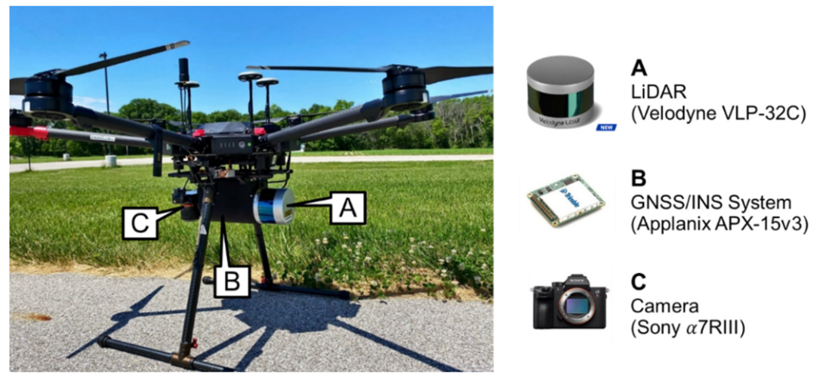
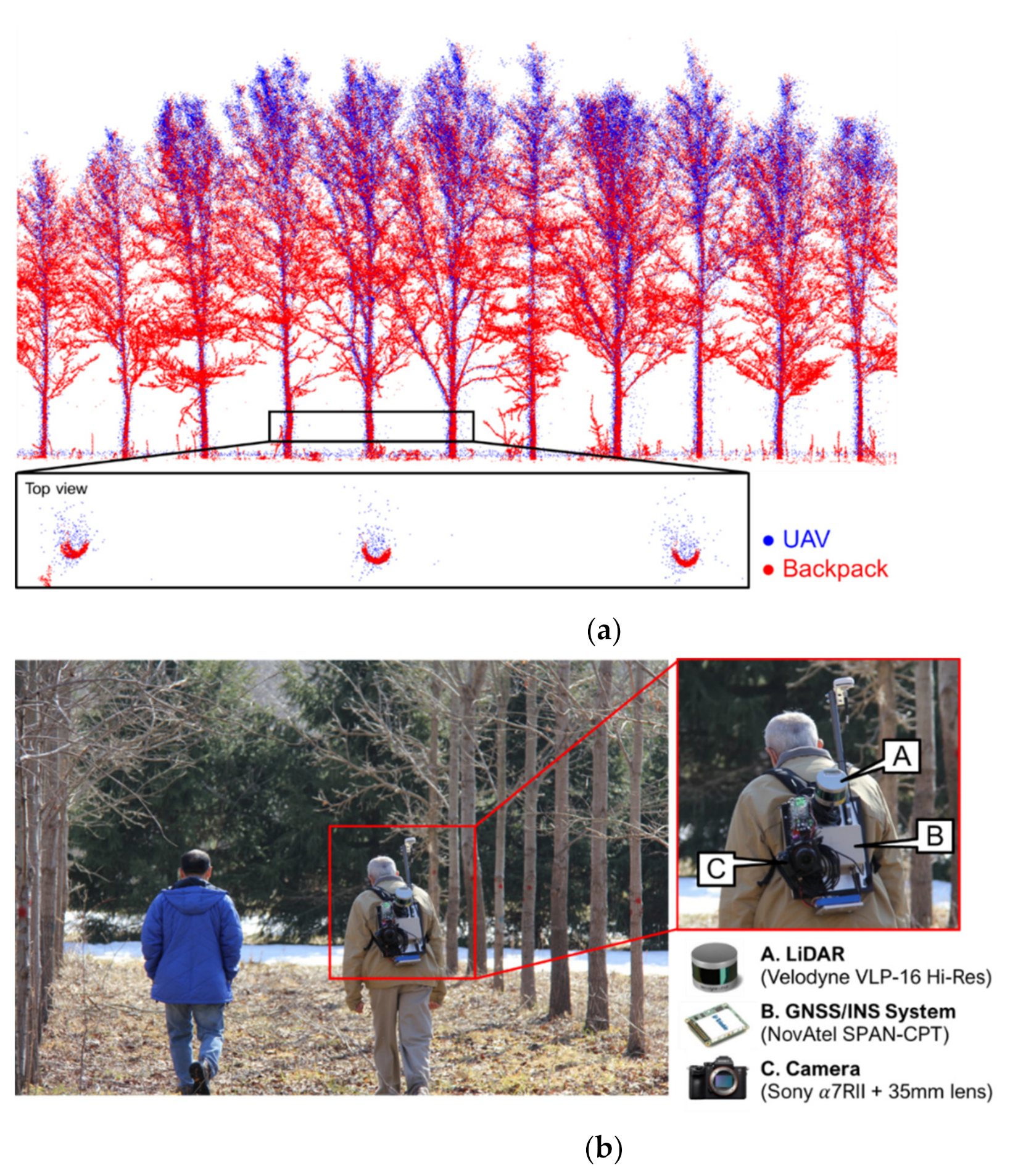
2.1. System Description and Calibration

The UAV (shown in Figure 1) payload consists of a Velodyne VLP-32C LiDAR and a Sony α7R III 43.6 MP full-frame camera with a 35 mm lens. The LiDAR and camera sensors are directly georeferenced by an Applanix APX15v3 position and orientation unit integrating a global navigation satellite system/inertial navigation system (GNSS/INS). The VLP-32C scanner is a spinning multi-beam LiDAR unit that has 32 radially oriented laser rangefinders. The vertical and horizontal field of view (FOV) relative to the rotation axis of the LiDAR unit is 40° (from +15° to −25°) and 360°, respectively. The scanner captures around 600,000 points per second (in single return mode), with a range accuracy of ±3 cm and a maximum range of 200 m [46]. For the GNSS/INS unit, the expected post-processing positional accuracy is ±2 to ±5 cm, and the attitude accuracy is ±0.025° and ±0.08° for the roll/pitch and heading, respectively [47].

The UAV system is built in such a way that the rotation axis of the LiDAR unit is approximately parallel to the flying direction. The FOV across the flying direction was set to ±70° from nadir, i.e., a point is reconstructed only when the laser beam pointing direction is less than ±70° from nadir. One benefit of using a spinning multi-beam LiDAR unit is the unique scanning mechanism. With multiple laser beams rotating and firing along different directions, there is a higher chance for the LiDAR energy to penetrate foliage and map below-canopy features. It also mitigates occlusion problems since a location in the object space can be captured by multiple laser beams at different times. To take advantage of the unique scanning mechanism and reconstruct point clouds with a large swath across the flying direction, rigorous system calibration is a prerequisite. In this study, the in-situ system calibration proposed by Ravi et al. [48] was conducted to determine the relative position and orientation between the onboard sensors and the GNSS/INS unit (hereafter denoted as mounting parameters). The expected accuracy of the point cloud was estimated based on the accuracy of individual sensors and standard deviations of the mounting parameters (estimated from system calibration) using the LiDAR Error Propagation calculator developed by Habib et al. [49]. At a flying height of 50 m, the calculator suggests that the horizontal and vertical accuracy value are in the ±5–6 cm range at nadir position. At the edge of the swath, the horizontal accuracy would be about ±8–9 cm and the vertical accuracy would still be in the ±5–6 cm range.

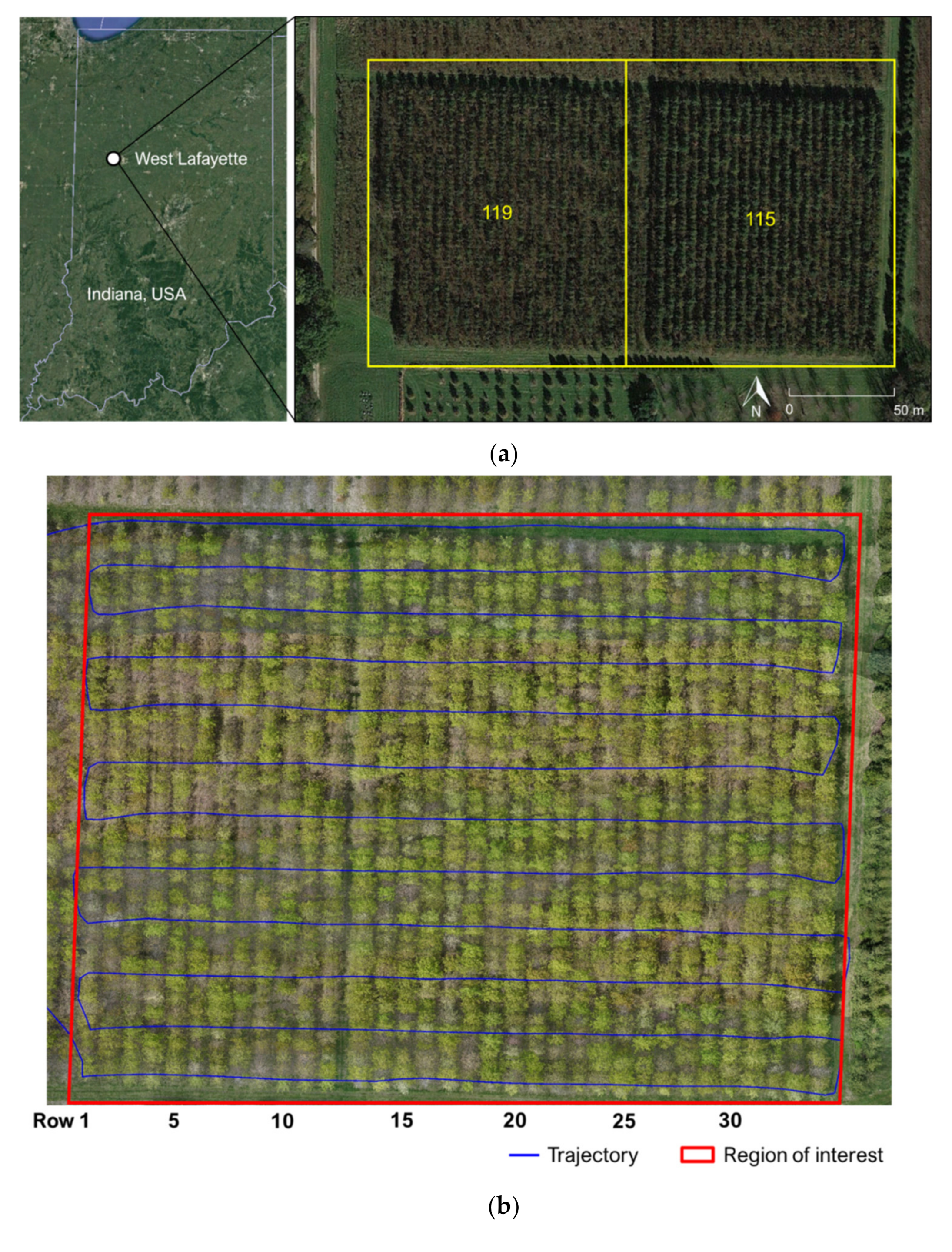
2.2. Study Site and Data Acquisition

Field surveys were carried out over a plantation in Martell forest, a forest owned by Purdue University, in West Lafayette, IN, USA (shown in Figure 2a). The study site consists of two plots, Plots 115 and 119 in Figure 2a, which were planted with northern red oak (Quercus rubra) as the primary species and burr oak (Q. macrocarpa) as trainers. Plots 115 and 119 were planted in 2007 and 2008, respectively, in a grid pattern: 22 rows in each plot and 50 trees in each row. The row spacing is approximately 5 m and the spacing between two adjacent trees in a row is approximately 2.5 m. The tree height ranges from 10 to 12 m at measurement year 13, and the branches interlace with each other. The average DBH is 12.7 cm and 11.3 cm in Plots 115 and 119, respectively. In terms of management, the understory vegetation, including herbaceous species and voluntary seedlings, has been controlled on an annual basis for Plot 115 (hereafter, denoted as the managed plot) but not Plot 119 (hereafter, denoted as the unmanaged plot).

Field surveys were conducted on 13 March 2021 (leaf-off), 11 May 2021 (partial leaf cover), and 2 August 2021 (full leaf cover).

Table 1. Flight configuration for datasets used in this study.

	13 March 2021	11 May 2021	2 August 2021
Number of flight lines	12	12	12
Flying height (m)	40	40	40
Lateral distance (m)	11	11	11
Ground speed (m/s)	3.5	3.5	3.5
Sidelap percentage (%)	95	95	95
Duration (s)	650	661	655
Number of images captured	451	465	484

reports the flight configuration for the three datasets, where the sidelap percentage was calculated according to a FOV of 140° across the flying direction. Figure 2b shows a sample orthophoto (from the May dataset) together with the UAV trajectory. The UAV flight line covers an area of approximately 2.5 ha. This area, as marked by the red box in Figure 2b, is the region of interest (ROI) for subsequent analyses. The ROI contains 34 rows, including 12 rows in Plot 119 (ground vegetation was not managed) and 22 rows in Plot 115 (ground vegetation was managed).

3. Methodology

This section introduces the data processing and analysis strategies, as outlined in Figure 3. There are three major components associated with the used strategies: (1) quality assessment of multi-temporal LiDAR data; (2) ground filtering and point cloud height normalization; and (3) individual tree segmentation. One should note that although the quality assessment has been listed as the first component, it relies on metrics derived from terrain and tree trunks, the second and third components, respectively. Therefore, this section begins by introducing the ground filtering and point cloud height normalization approaches. Next, the proposed tree detection and segmentation approach is presented in Section 4.2. Finally, Section 4.3 describes the point cloud quality assessment.

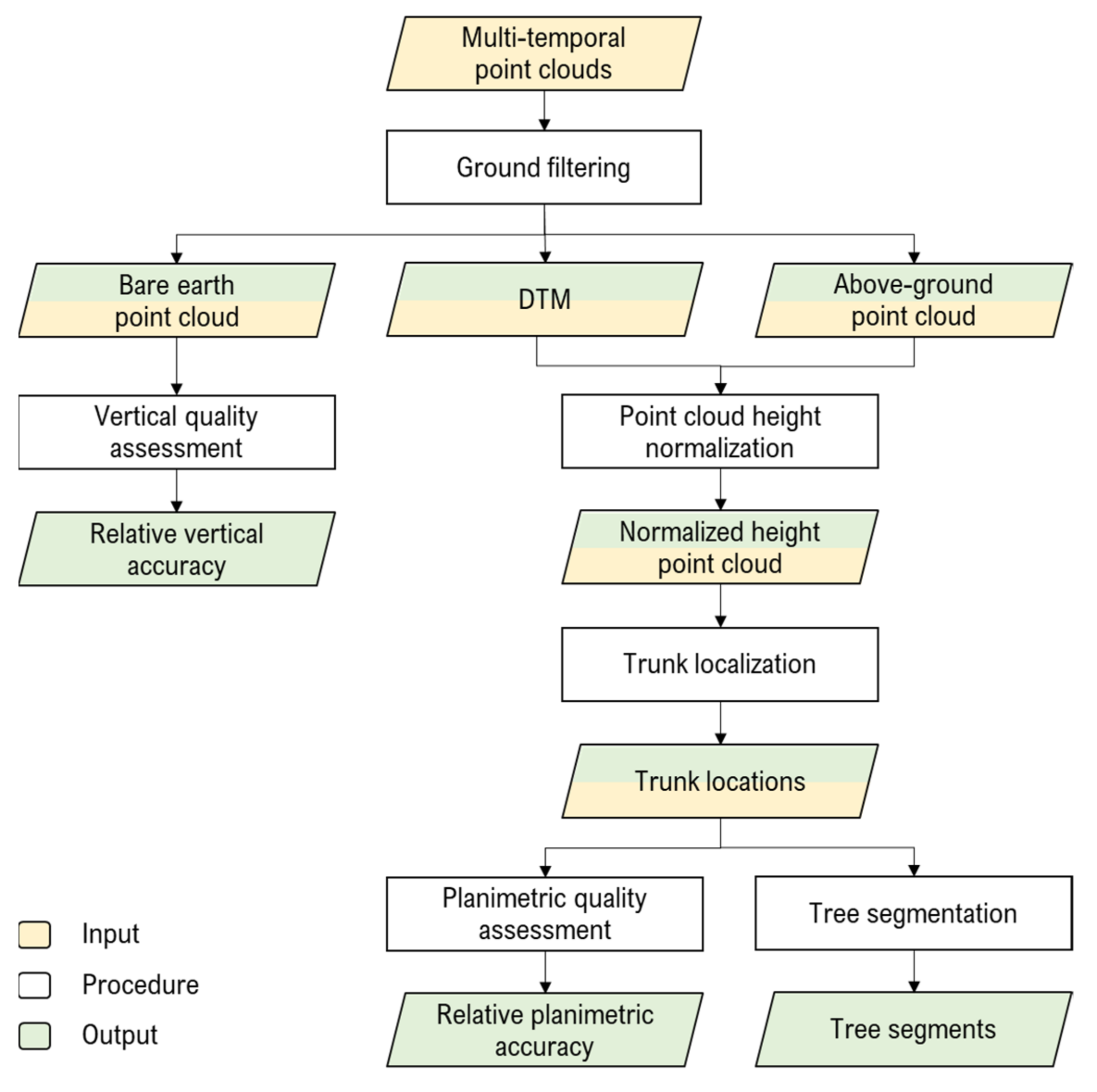
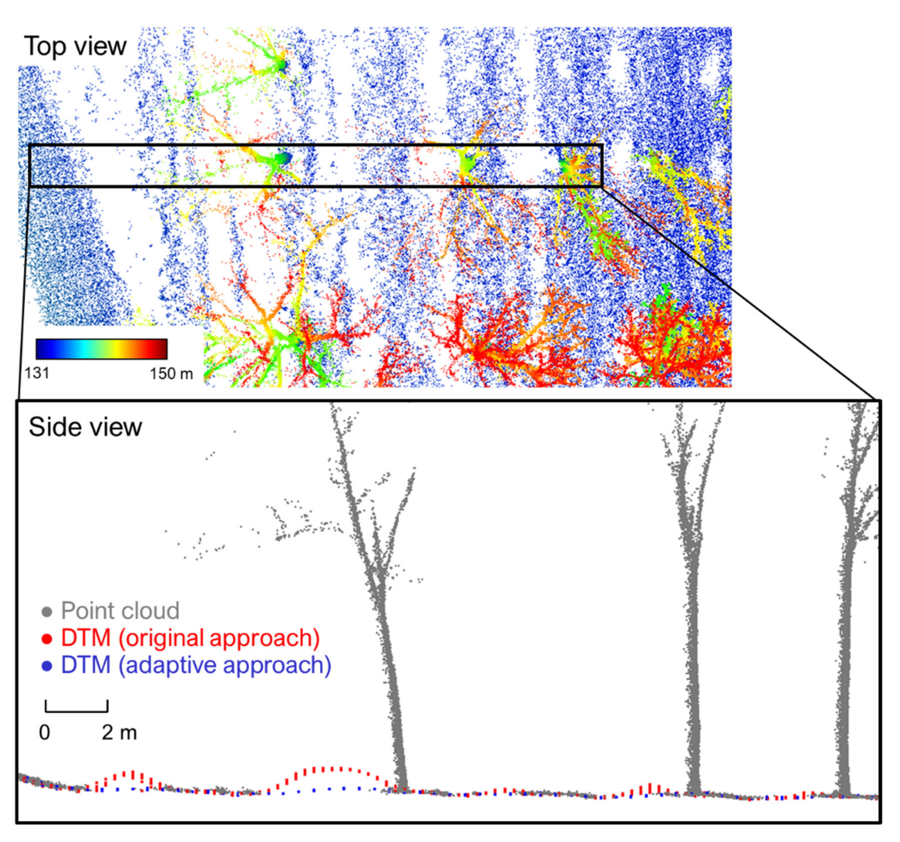
3.1. Ground Filtering and Point Cloud Height Normalization

Upon reconstructing the point cloud, a ground filtering algorithm is used to separate bare earth points (which represent the terrain) from above-ground points and subsequently generate a rasterized DTM. In this study, the adaptive cloth simulation algorithm proposed by Lin et al. [50] is adopted. First, the original cloth simulation approach [51] is performed to extract an initial bare earth point cloud. The conceptual basis of the original cloth simulation approach can be summarized as follows: (1) turn the point cloud upside down, (2) define a cloth (consisting of particles and their interconnections) with some rigidness and place it above the point cloud, (3) let the cloth drop under the influence of gravity and designate the final shape of the cloth as the DTM, and (4) use the DTM to filter the ground from above-ground points [51]. For the adaptive approach, the rigidness of each particle on the cloth is redefined based on the point density of an initially established bare earth point cloud. The cloth simulation is applied again to obtain a refined bare earth point cloud and the final DTM. By modifying the rigidness of the cloth based on the point density, the adaptive approach can generate a reliable DTM even with sparse bare earth points [50]. An example of a DTM generated based on the original and adaptive approaches is illustrated in Figure 4. The cross-sectional profile side view highlights the observable difference between the two DTMs. As can be seen in the figure, in areas with sparse point cloud the DTM from the adaptive approach is more reliable when compared to that from the original approach.

Following ground filtering, the above-ground point cloud is normalized by subtracting the corresponding ground elevation (based on the generated DTM) from each above-ground point. After normalization, the height value of a point would represent the elevation above ground. Figure 5 shows a sample above-ground point cloud before and after height normalization. The elevation values in Figure 5a,b are the ellipsoidal height and height above ground, respectively. The former is relative to a reference ellipsoid that approximates the Earth surface; the latter is relative to the ground and therefore can be used to evaluate the tree height. In this study, the normalized height above-ground point cloud is used for tree localization and segmentation.

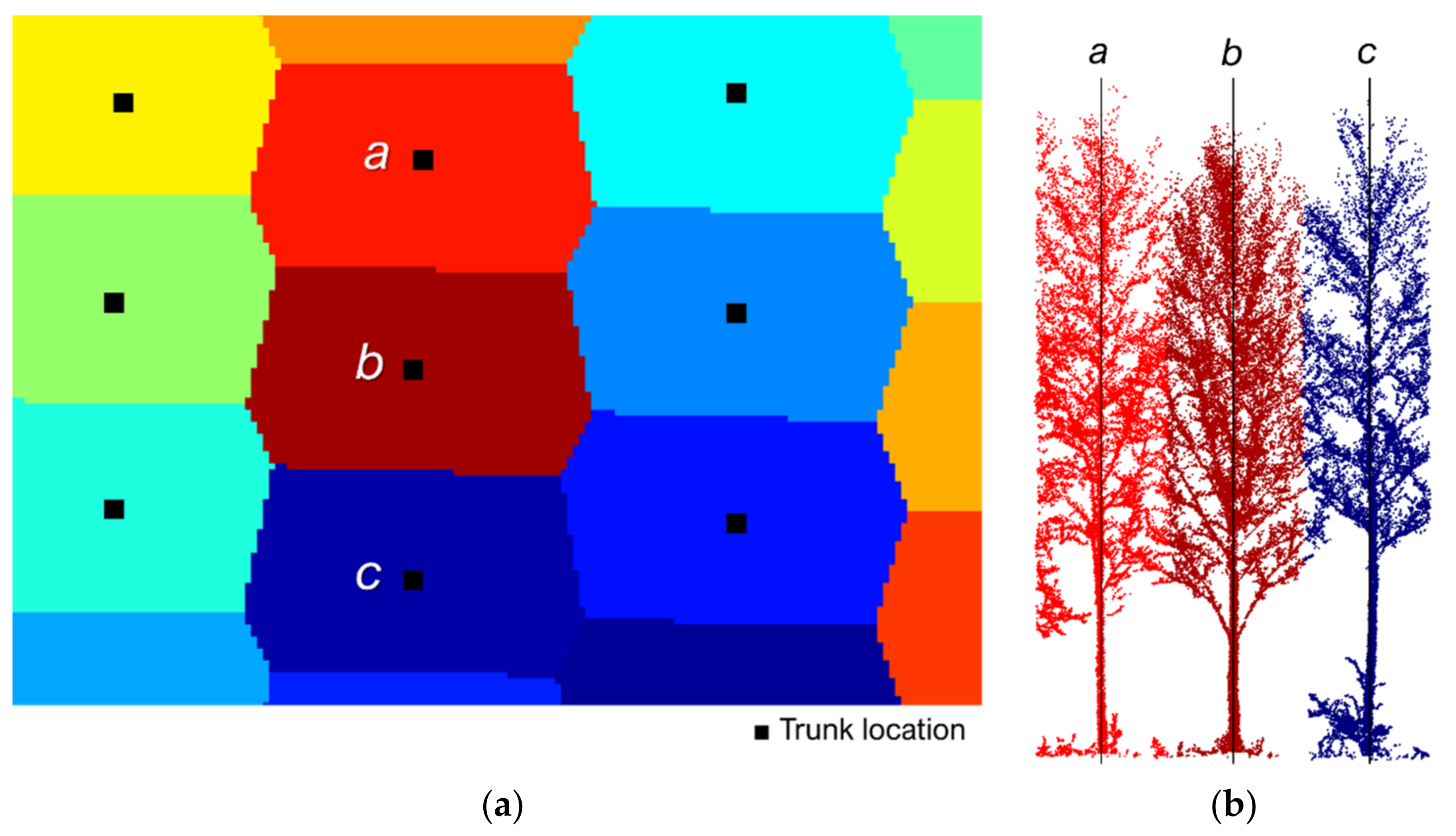
3.2. Tree Localization and Segmentation

In this study, a bottom-up approach is proposed for localization and segmentation of individual trees from the point cloud. The proposed approach first detects the trunks using the normalized height above-ground point cloud. An advantage of the proposed approach is that it provides the planimetric locations of the trunks. Individual trees are then segmented based on the detected trunk locations. The reason for choosing a bottom-up approach is based on the observation that the UAV LiDAR can penetrate through canopy and capture tree trunks and ground. Also, unlike canopies which tend to overlap with each other, trunks are naturally separated from each other and therefore easier to identify.

The proposed trunk localization strategy is based on the hypothesis that higher point density and higher elevation correspond to trunk locations. First, a point cloud that roughly corresponds to the understory layer is extracted from the normalized height above-ground point cloud based on user-defined minimum and maximum height thresholds, as illustrated in Figure 6. As a result, the majority of the canopy and shrub are removed and only the point cloud portion pertaining to the trunks is retained. Next, two-dimensional cells are created along the XY plane over the region of interest (ROI). For each cell, the sum of elevations of all points is evaluated. This metric reflects the point density and height of the point cloud in a local neighborhood. A 2D peak detection is then carried out to identify local maxima of the metric, which would correspond to the trunk locations. Two parameters are involved in the peak detection: size of the local neighborhood and minimum prominence of a peak. The former can be selected according to prior information about the field, i.e., approximate trunk diameter and tree spacing. The latter needs to be tuned for each dataset since it relates to point density, which depends on technical factors pertaining to data acquisition such as the pulse repetition rate of the LiDAR unit, flying height, ground speed, and overlap percentage. A sample trunk localization result showing the top and side views of the normalized height above-ground point cloud together with detected 2D trunk locations is depicted in Figure 6.

The performance of the trunk localization algorithm is evaluated using manually identified ground truth. The manual tree identification is carried out by examining the point cloud over the ROI and manually identifying all the tree locations. The manually established trunk locations are expected to have a cm-level accuracy considering the noise level of the point cloud. Precision, recall, and F1-score–as represented by Equations (1)–(3) where TP, FP, and FN are the true positives, false positives, and false negatives, respectively–are used to quantify the performance of trunk detection. Precision signifies how relevant the positive detections are, recall indicates how well the actual trees are identified, and F1-score quantifies the overall performance. In addition, for the true positives, the planimetric differences between the detected trunk locations and corresponding ground truth are calculated and the mean, standard deviation, and root-mean-square error (RMSE) are reported.

$$\mathrm{Precision}=\frac{\mathrm{TP}}{\mathrm{TP}+\mathrm{FP}}$$

(1)

$$\mathrm{Recall}=\frac{\mathrm{TP}}{\mathrm{TP}+\mathrm{FN}}$$

(2)

$$\mathrm{F}1\mathrm{score}=2\times \frac{\mathrm{Precision}\times \mathrm{Recall}}{\mathrm{Precision}+\mathrm{Recall}}$$

(3)

Once the trunks are identified, individual trees are segmented from the normalized height above-ground point cloud based on the trunk locations and distance. The conceptual basis of the proposed tree segmentation approach is that for every point in a tree segment, its planimetric distance to the corresponding trunk is smaller than that to any other trunk. A 2D Voronoi diagram is established along the XY plane using the trunk locations as seeds–refer to the graphical illustration in Figure 7. The normalized height above-ground point cloud is then segmented based on the Voronoi diagram.

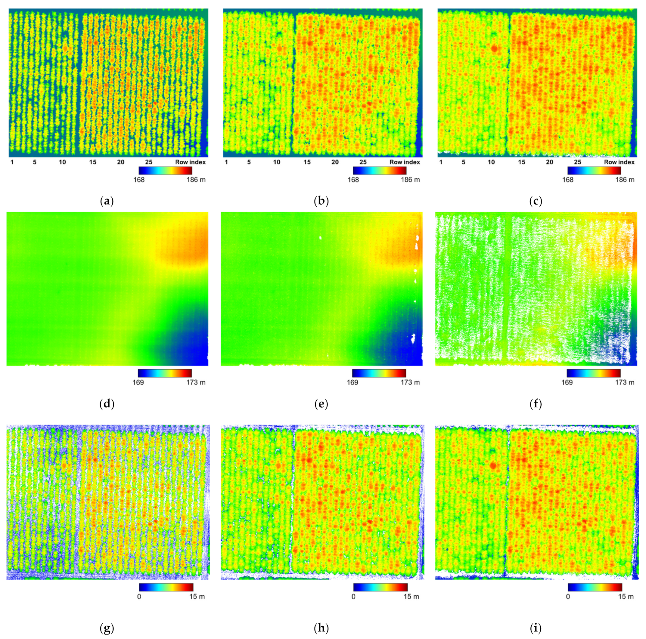
3.3. Point Cloud Quality Assessment

The quality assessment strategy proposed by Lin and Habib [52] is adopted for evaluating the relative accuracy of the point clouds, namely, the alignment between multi-temporal point clouds. The approach utilizes points/features that remain stable throughout time and can be automatically identified and extracted from the point cloud data. No target deployment is required. In this study, the trunks and terrain patches are used as 2D points and planar features, respectively, for evaluating the relative accuracy of multi-temporal point clouds.

The trunk locations, detected using the approach described in Section 3.2, are 2D points that provide discrepancy information among temporal datasets along the X and Y directions. Conjugate trunks among multi-temporal point clouds are paired by searching for the nearest trunk within a given search radius. The search radius is defined by the approximate tree spacing. Upon establishing the trunk correspondence, the planimetric discrepancy between conjugate trunks (${\left[\begin{array}{cc}{d}_{x\_obs}& d_{y\_obs}\end{array}\right]}^T$) can be calculated. The least squares adjustment (LSA) for estimating the net planimetric discrepancy between two point clouds using trunk locations can be written as per Equation (4). In the equation, ${\left[\begin{array}{cc}{d}_x& d_y\end{array}\right]}^T$ denotes the net planimetric discrepancy between two point clouds; the random noise ${\left[\begin{array}{cc}{e}_x& e_y\end{array}\right]}^T$ follows a stochastic distribution with a zero mean and variance-covariance matrix ${\sigma }_0^2{P}^{-1}$, where ${\sigma }_0^2$ is the a-priori variance factor and $P$ is the weight matrix.

$$\left[\begin{array}{c}{d}_{x\_obs}\\ d_{y\_obs}\end{array}\right]=\left[\begin{array}{c}{d}_x\\ d_y\end{array}\right]+\left[\begin{array}{c}{e}_x\\ e_y\end{array}\right], e~\left(0,{\sigma }_0^2{P}^{-1}\right)$$

(4)

The terrain patches are planar patches segmented from the bare earth point clouds with a pre-determined size based on the approach described in Lin and Habib [52]. The discrepancy between conjugate patches can be written as ${\left[\begin{array}{ccc}{d}_{x\_obs}& d_{y\_obs}& d_{z\_obs}\end{array}\right]}^T$. On should note that although the discrepancy has three components, a planar feature provides discrepancy information only along the normal direction to the plane. This leads to the need of incorporating a modified weight matrix in the LSA model [53]. The LSA model for net discrepancy estimation using terrain patches is given by Equation (5). The discrepancies between conjugate terrain patches are direct observations of the net discrepancy between two point clouds (${\left[\begin{array}{ccc}{d}_x& d_y& d_z\end{array}\right]}^T$). The random noise ${\left[\begin{array}{ccc}{e}_x& e_y& e_z\end{array}\right]}^T$ has a mean of zero and variance-covariance matrix of ${\sigma }_0^2{P}_{xyz}^{\prime }{}^{+}$, with ${\sigma }_0^2$ is the a-priori variance factor and $P_{xyz}^{\prime }$ is the modified weight matrix. The plus sign denotes the Moore–Penrose pseudoinverse since $P_{xyz}^{\prime }$ is rank-deficient and its inverse does not exist. One should note that although the least squares adjustment evaluates the discrepancies along the X, Y, and Z directions, the reliability of these estimates depends on the variation in the orientation/slope/aspect within the region of interest. In the study site, the terrain is mostly flat or has a mild slope, and thus provides discrepancy information mainly along the vertical direction. Therefore, only the vertical discrepancy estimation is reported.

$$\left[\begin{array}{c}{d}_{x\_obs}\\ d_{y\_obs}\\ d_{z\_obs}\end{array}\right]=\left[\begin{array}{c}{d}_x\\ d_y\\ d_z\end{array}\right]+\left[\begin{array}{c}{e}_x\\ e_y\\ e_z\end{array}\right], e~\left(0,{\sigma }_0^2{P}_{xyz}^{\prime }{}^{+}\right)$$

(5)

4. Experimental Results

The datasets acquired in March (leaf-off), May (partial leaf cover), and August (full leaf cover) were used to evaluate the agreement among multi-temporal datasets, level of detail captured by UAV LiDAR, and performance of the proposed tree localization and segmentation approach under different leaf cover scenarios and management practices in forest plantation. The quality assessment is presented lastly in Section 4.3 since it relies on features derived from the point clouds–terrain (covered in Section 4.1) and tree locations (introduced in Section 4.2).

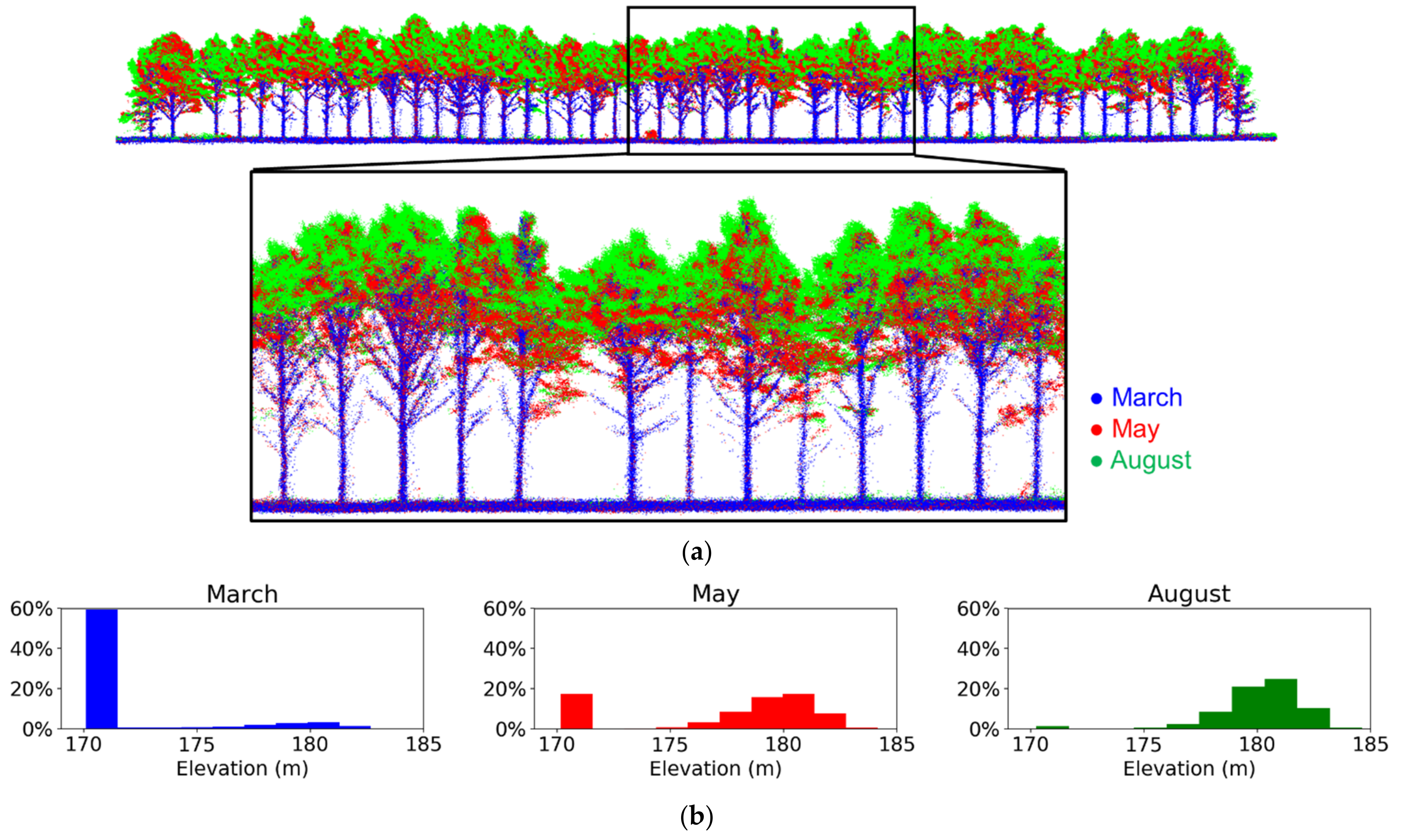
4.1. UAV LiDAR Data under Different Leaf Cover Scenarios

Point clouds acquired under different leaf cover scenarios were examined using the March (leaf-off), May (partial leaf cover), and August (full leaf cover) datasets. The adaptive cloth simulation algorithm was applied to separate the bare earth and above-ground points and generate DTMs. The above-ground point clouds were then normalized by subtracting the ground elevation based on the DTM. Figure 8 shows top view of the original, bare earth, and normalized height above-ground point clouds from the three datasets. The increase in canopy cover can be observed from the original and normalized height above-ground point clouds. The bare earth point clouds, in contrast, display similar spatial patterns, showing that the terrain remained stable between the three surveys.

To further inspect the point cloud, we manually cropped a row (Row 16 in Figure 8a) from the point cloud and examined its side view, as depicted in Figure 9. As shown in the figure, terrain was captured by UAV LiDAR in all three datasets. Tree trunks, on the other hand, were captured in March (leaf-off) and May (partial leaf cover), but not in August (full leaf cover). One can also observe individual tree mortality at locations i and ii according to the planting pattern (50 trees in each row), as noted in Figure 9a. Having established the mounting parameters for the camera and LiDAR units, the images covering location i and ii were identified and shown in Figure 9b,c. The missing trees can be identified based on the images under leaf-off condition. Figure 10a shows Row 16 from the March (leaf-off), May (partial leaf cover), and August (full leaf cover) datasets superimposed on top of each other. Qualitatively, the multi-temporal point clouds are in good agreement since the terrain and tree trunks are well-aligned. The point cloud under leaf-off condition provides more coverage of the terrain and tree trunks; in contrast, the majority of the points from leaf-on surveys captures foliage. This observation can be verified through the elevation histogram that quantifies the vertical distribution of the points, as illustrated in Figure 10b.

Table 2. Summary of point cloud characteristics for the LiDAR datasets.

Dataset	Number of Points (Million)			Percentage (%)
	Total	Bare Earth	Above-Ground	Bare Earth	Above-Ground
March (leaf-off)	143.7	121.4	22.3	84	16
May (partial leaf cover)	116.2	40.8	75.4	35	65
August (full leaf cover)	112.6	7.5	105.1	7	93

reports a summary of point cloud characteristics, including the number of points and percentage of the original, bare earth, and above-ground point clouds. The quantitative results suggest that the majority of points (84% of the points) could reach the terrain under the leaf-off condition. Under the partial and full leaf cover conditions, more points were capturing the canopy and only 35% and 7% of the points, respectively, were able to reach the terrain. Although the number of bare earth points reduced significantly, the bare earth point clouds were dense enough for generating reliable DTMs; this could also be observed from Figure 8e,f. The point density of the original and bare earth point clouds over the surveyed area was evaluated based on a uniform 2D grid and visualized as a grayscale map, as shown in Figure 11. The statistics of point density, including the 25th percentile, median, and 75th percentile in the surveyed area, are reported in

Table 3. Statistics of the point density of the original and bare earth point clouds in the ROI.

	Dataset	Point Density (Points/m2)
		25th Percentile	Median	75th Percentile
Original point cloud	March (leaf-off)	1000	3600	5500
	May (partial leaf cover)	1100	2500	4500
	August (full leaf cover)	1000	2500	4600
Bare earth point cloud	March (leaf-off)	900	3300	4900
	May (partial leaf cover)	600	1100	1700
	August (full leaf cover)	100	200	600

. In this study, the flight configurations for the three field surveys were identical and the tree density in the plantation remained the same. Therefore, the variation in point density was mainly affected by the canopy cover.

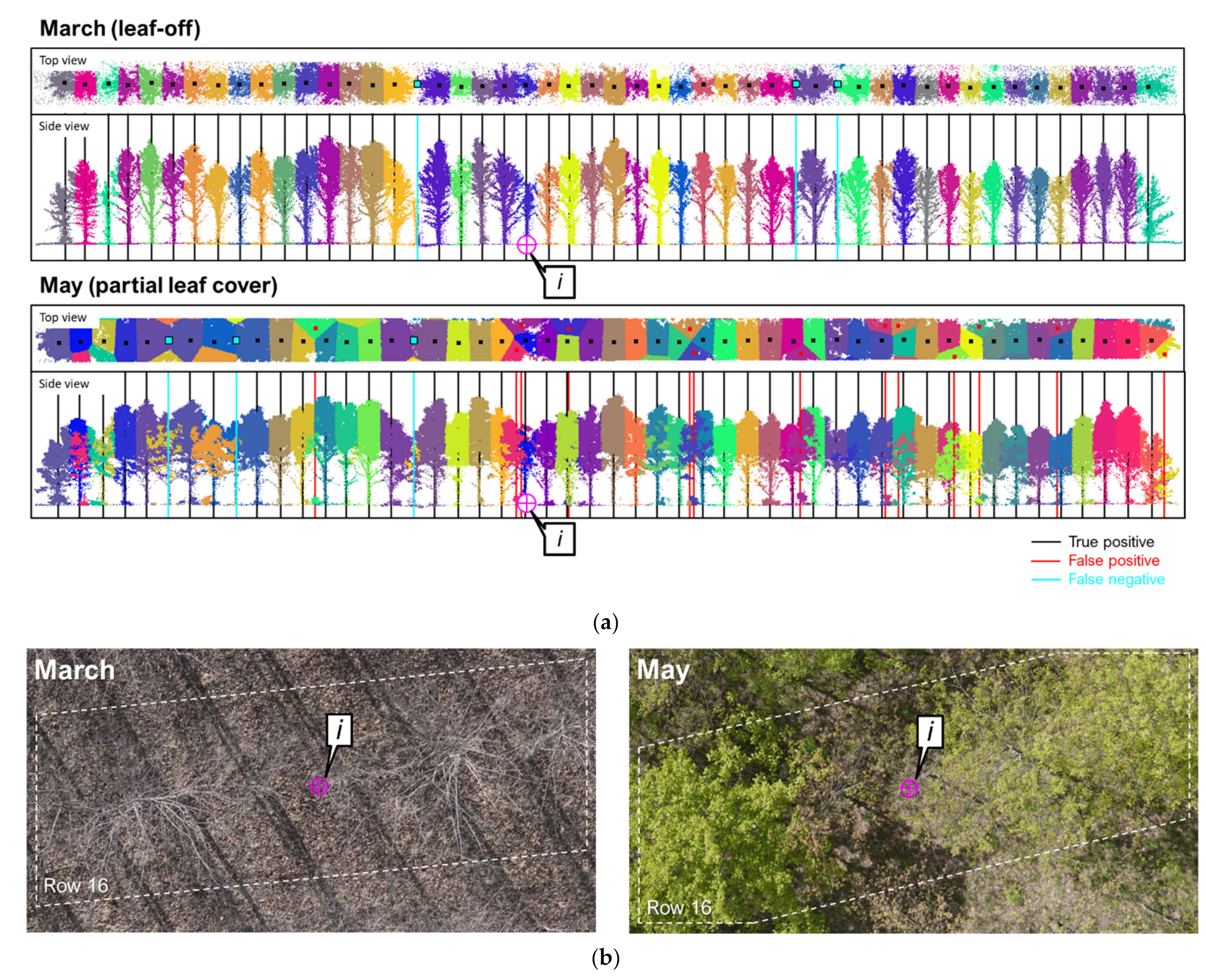
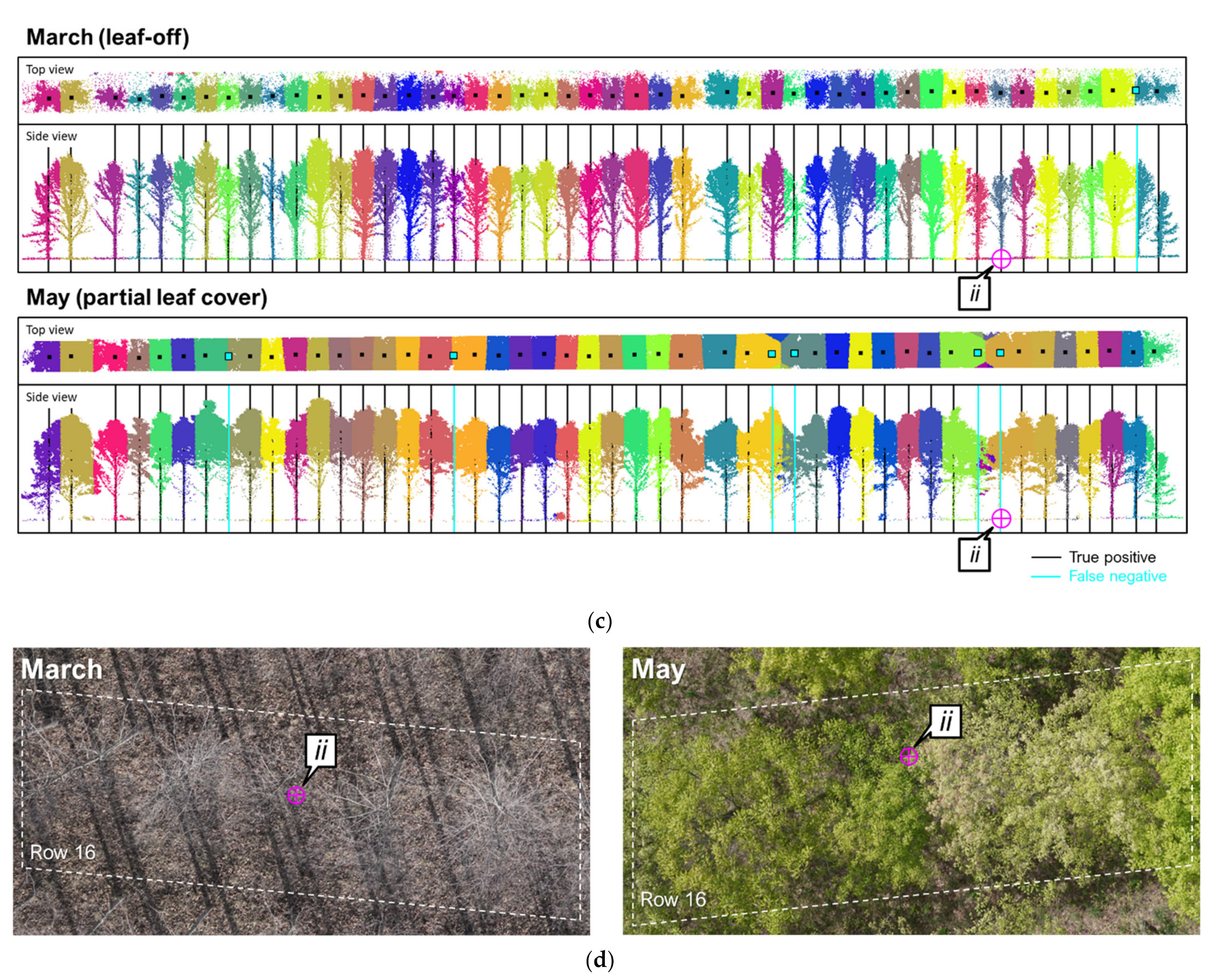
4.2. Tree Localization and Segmentation Results for Different Leaf Cover Scenarios

The proposed tree localization and segmentation approach was tested using the normalized height above-ground point cloud from March (leaf-off), May (partial leaf cover), and August (full leaf cover) datasets. For trunk localization, the maximum and minimum height thresholds for extracting understory layers from the normalized height above-ground point cloud were set to 0.5 and 2.5 m, respectively. The cell size for evaluating the sum of elevations of all points in a cell was set to 10 cm. The size of the local neighborhood for peak detection was set to 1 × 1 m.

The proposed trunk localization approach was compared against the DBSCAN, a clustering algorithm that was adopted by prior research for trunk detection [18,45]. The performance of the two algorithms was evaluated using manually established ground truth and reported in

Table 4. Performance of the proposed trunk localization approach and DBSCAN clustering evaluated for the March (leaf-off), May (partial leaf cover), and August (full leaf cover) datasets.

		March			May			August
		Plot 119	Plot 115	Total	Plot 119	Plot 115	Total	Plot 119	Plot 115	Total
	Total number of trees	585	1080	1665	585	1080	1665	585	1080	1665
Proposed approach	True positive	567	1034	1601	539	923	1462	0	0	0
	False positive	0	0	0	151	29	180	2	2	2
	False negative	18	46	64	46	157	203	585	1080	1665
	Precision	1.00	1.00	1.00	0.78	0.97	0.89	0.00	0.00	0.00
	Recall	0.97	0.96	0.96	0.92	0.85	0.88	0.00	0.00	0.00
	F1 score	0.98	0.98	0.98	0.85	0.91	0.88	N/A	N/A	N/A
DBSCAN	True positive	584	1078	1662	524	853	1377	8	1	9
	False positive	6	0	6	225	45	270	291	91	382
	False negative	1	2	3	61	227	288	577	1079	1656
	Precision	0.99	1.00	1.00	0.70	0.95	0.84	0.03	0.01	0.02
	Recall	1.00	1.00	1.00	0.90	0.79	0.83	0.01	0.00	0.01
	F1 score	0.99	1.00	1.00	0.79	0.86	0.83	0.02	0.00	0.01

. The results suggest that the proposed approach provided a performance similar to the DBSCAN under leaf-off condition (the F1-score is 0.98 and 1.00 for the former and latter, respectively). Under partial leaf cover condition, the proposed approach achieved an F1-score of 0.88, outperforming the DBSCAN that had an F1-score of 0.83. Both the proposed approach and DBSCAN failed to detect tree locations under full leaf cover condition because trunks were not captured in the point cloud, as can be seen in Figure 9a. However, the false positives from the proposed algorithm were much lower than that from the DBSCAN–only two false positives from the former as opposed to 382 from the latter. In terms of management practices, both algorithms delivered a higher precision in the managed plot (Plot 115) whereas a higher recall in the unmanaged plot (Plot 119) was achieved. Overall, the consistently low false positive rate highlights the superior robustness of the proposed algorithm in handling noisy and sparse point clouds, which is particularly critical under leaf-on conditions.

In contrast to the DBSCAN strategy, which groups the points that belong to the same tree trunk, the proposed approach derives the planimetric locations of the trunk centers. The accuracy of the trunk localization results was assessed using the manually established ground truth.

Table 5. Trunk localization accuracy assessment using the March (leaf-off) and May (partial leaf cover) datasets showing the coordinate differences ($d_x$ and $d_y$ ) between the detected trunk location and ground truth.

		Plot 119		Plot 115		Total
		${\mathit{d}}_{\mathit{x}}\left(\mathbf{m}\right)$	${\mathit{d}}_{\mathit{y}}\left(\mathbf{m}\right)$	${\mathit{d}}_{\mathit{x}}\left(\mathbf{m}\right)$	${\mathit{d}}_{\mathit{y}}\left(\mathbf{m}\right)$	${\mathit{d}}_{\mathit{x}}\left(\mathbf{m}\right)$	${\mathit{d}}_{\mathit{y}}\left(\mathbf{m}\right)$
March (leaf-off)	Mean	0.02	0.02	−0.02	0.01	−0.01	0.01
	Std. Dev.	0.08	0.07	0.08	0.07	0.08	0.07
	RMSE	0.08	0.08	0.08	0.07	0.08	0.07
May (partial leaf cover)	Mean	0.01	0.02	−0.02	0.02	−0.01	0.02
	Std. Dev.	0.12	0.08	0.08	0.09	0.10	0.09
	RMSE	0.12	0.08	0.09	0.09	0.10	0.09

reports the mean, standard deviation, and RMSE of the coordinate differences between the true positives from the proposed algorithm and manually established ground truth. One should note that the August (full leaf cover) dataset was not included in the analysis since there was no true positive from the proposed algorithm (refer to Table 4). The result suggests that the tree localization achieved an accuracy of 0.1 m regardless of leaf-off and partial leaf cover scenarios and management practices. This accuracy depends mostly on the cell size for peak detection using the sum of elevations metric.

To provide a closer view of the tree detection and segmentation results using the proposed approach, Figure 12 shows top and side views of the point cloud and detected tree locations for row 11 in Plot 119 (unmanaged) and Row 16 in Plot 115 (managed). One should note that the point cloud from the August (full leaf cover) dataset is not included in the figure since it barely captures the trunks, as can be observed in Figure 9a. In the figure, the correct detections (true positive) are shown in black, the commission errors (false positive) are shown in red, and the omission errors (false negative) are shown in cyan. Sample images capturing the locations where the algorithm fails are also shown in Figure 12. According to the point cloud side view shown in Figure 12, the correct detections align well with the trunks. The results suggest that omission errors tend to happen for small or undeveloped trees, or in areas with dense canopy where the point cloud is too sparse over the trunk. Omission errors are found in both leaf-off and partial leaf cover conditions, yet are more common in the latter scenario. Commission errors happened mostly because of the shrubs, branches, and leaves that were not excluded by the height thresholds. Therefore, commission errors are higher under partial leaf cover condition and in unmanaged plot.

4.3. Quantitative Relative Quality Assessment of Multi-Temporal Point Clouds

The alignment between point clouds from the March (leaf-off), May (partial leaf cover), and August (full leaf cover) datasets was evaluated quantitatively using the quality assessment approach described in Section 3.3. The relative planimetric discrepancies between point clouds were estimated using the detected trunk locations. The August dataset was not included in this analysis because the trunks were not captured in the point cloud.

Table 6. Estimated horizontal discrepancy ($d_x$ and $d_y$ ) and square root of a posteriori variance ($\widehat{{\sigma }_0}$ ).

Reference	Source	Number of Observations	$\widehat{{\mathit{\sigma }}_0}\left(\mathbf{m}\right)$	${\mathit{d}}_{\mathit{x}}\left(\mathbf{m}\right)$		${\mathit{d}}_{\mathit{y}}\left(\mathbf{m}\right)$
				Parameter	Std. Dev.	Parameter	Std. Dev.
March (leaf-off)	May (partial leaf cover)	1538	0.085	0.011	0.002	−0.006	0.002

reports the square root of a-posteriori variance factor ($\widehat{{\sigma }_0}$) and the estimated planimetric discrepancy ($d_x$ and $d_y$) between the point clouds from March and May surveys. The former reflects the accuracy of the detected trunk locations, and the latter signifies the overall net discrepancy between the point clouds in question. The square root of a-posteriori variance factor suggests a trunk detection accuracy of ±9 cm, which is in agreement with the 10 cm cell size used for evaluating the peak detection metric (i.e., sum of elevations). The discrepancy estimation, based on 1538 detected and paired trunk locations, suggests that the two datasets are compatible within a 1 cm range in both the X and Y directions. The relative vertical discrepancy between point clouds was estimated using terrain patches extracted from the bare earth point clouds. The size of the terrain patches was set to 1.5 m × 1.5 m. The square root of a-posteriori variance factor ($\widehat{{\sigma }_0}$) and the estimated vertical discrepancy ($d_z$) between the point clouds are reported in

Table 7. Estimated vertical discrepancy ($d_z$ ) and square root of a posteriori variance ($\widehat{{\sigma }_0}$ ).

Reference	Source	Number of Observations	$\widehat{{\mathit{\sigma }}_0}\left(\mathbf{m}\right)$	${\mathit{d}}_{\mathit{z}}\left(\mathbf{m}\right)$
				Parameter	Std. Dev.
March (leaf-off)	May (partial leaf cover)	11,918	0.021	0.011	1.91 $\times {10}^{-4}$
March (leaf-off)	August (full leaf cover)	11,098	0.071	0.109	6.75 $\times {10}^{-4}$

. The square root of a-posteriori variance factor reflects the noise level of the point clouds. The discrepancy estimation shows that the point clouds are in agreement within a 1 cm and 11 cm range along the vertical direction between March and May, and March and August, respectively. Overall, the relative quality assessment results verify that the point clouds from leaf-off and partial leaf cover conditions exhibit a good degree of agreement with an overall precision of ±1 cm. Possible reasons behind the large discrepancy between March and August datasets could be: (1) the sparse bare earth point cloud in August, which mainly capture the top of terrain and/or understory vegetation and (2) the growth of below-canopy plants.

5. Discussion

This study investigated the capability of UAV LiDAR in mapping below-canopy features including terrain and tree trunks under different leaf cover conditions and management practices in a forest plantation. The results show that the terrain was captured in all three datasets. Although the point density of the bare earth point cloud decreases as the leaf cover increases, the terrain models derived from the three datasets are comparable. Consequently, the normalized height above-ground point clouds, which are essential for deriving canopy height, can be reliably generated. Tree trunks, on the other hand, were captured in March (leaf-off) and May (partial leaf cover), but not in August (full leaf cover) due to the dense canopy cover. Prior research mapped tree trunks using LiDAR data from above-canopy flights under leaf-off condition [44], below-canopy UAV flights [45], and ground systems (TLS and ground mobile LiDAR) [18]. This study reveals the potential of mapping tree trunks using above-canopy UAV-LiDAR flights under partial leaf cover conditions.

A bottom-up tree localization and segmentation approach was proposed and compared against the density-based clustering algorithm, DBSCAN, that has been adopted by other previous studies for trunk detection [18,45]. The experimental results show that the proposed approach can detect tree locations with accuracy similar to that from DBSCAN under the leaf-off condition. Under partial leaf cover conditions, the proposed approach outperformed the DBSCAN. Under full leaf cover, both approaches could not detect the trunks. Nevertheless, the low false positive rate from the proposed approach reveals its superior robustness against noisy and sparse point clouds, especially under leaf-on condition. Moreover, the proposed approach delivers planimetric locations of the tree trunks in contrast to DBSCAN that only provides detection. Overall, the success of this study in detecting terrain and trunks can be attributed to the following reasons:

• Rigorous system calibration ensures the quality of multi-temporal LiDAR point clouds. It is also the key for reconstructing a large swath across the flying direction, which leads to the high side-lap percentage and thus high point density of the derived point cloud.
• The proposed trunk localization approach utilizes both point density and height. Compared to the DBSCAN that solely relies on point density, it is more reliable when dealing with noisy and sparse point clouds.

Finally, the ability of LiDAR in deriving structural information of individual trees depends on the noise level in the point cloud. Figure 13 displays a UAV LiDAR point cloud from this study (using the March dataset under leaf-off condition) overlapped with a point cloud acquired by a Backpack system equipped with a Velodyne VLP16 Hi-Res integrated with a GNSS/INS unit. The VLP16 Hi-Res unit has 16 laser beams, which is fewer than the 32 laser beams of the VLP-32C scanner onboard the UAV system. Although the Velodyne LiDAR units has similar range accuracy, the point cloud form the Backpack system has a much lower noise level because of the short object-to-sensor distance. Consequently, the point cloud from the Backpack system can capture finer details such as the circular shape of the trunk cross-section as depicted in Figure 13a. Also, one can see in Figure 13a the capability of aerial and ground systems to map different parts of the forest vertical structure owing to their distinct view angles. The top portion of the canopy is better described by the UAV data while the intermediate and low parts of the forest is better mapped by the Backpack data.

6. Conclusions and Future Work

This paper presented an evaluation and application of UAV LiDAR for single-tree inventory in forest plantations. The quality of UAV LiDAR mapping products under different leaf cover scenarios were evaluated. A bottom-up tree localization and segmentation approach based on 2D peak detection and a Voronoi diagram was proposed and compared against an existing density-based clustering algorithm. Field surveys were carried out at a forest plantation under leaf-off, partial leaf cover, and full leaf cover conditions. Quality assessment results indicate that multi-temporal point clouds were in good agreement within a 1-to-10 cm range. While the percentage of bare earth points reduced from 84%, 35%, to 7%, the DTMs corresponding to the three scenarios were comparable; consequently, normalized height above-ground point clouds could be derived reliably. The proposed trunk detection algorithm achieved an F1-score of 0.98 and 0.88 under lead-off and partial leaf cover conditions, respectively. Both the proposed approach and the density-based clustering algorithm failed to detect tree trunks under the full leaf cover condition. Overall, the proposed approach outperformed the density-based clustering algorithm due to its superior robustness against noisy and sparse point clouds, which is critical for handling UAV LiDAR data under the leaf-on condition. The detected tree locations achieved an accuracy of 0.1 m regardless of leaf-off and partial leaf cover scenarios and management practices.

There are several potential directions for future research. First, the performance of the proposed trunk detection algorithm will be tested in natural forests. A more robust and accurate tree segmentation approach will be also developed. Next, imagery data acquired by the UAV will be integrated with LiDAR data for tree species identification. Finally, the potential of fusing the UAV LiDAR data with ground systems to obtain detailed vertical structure information will be explored.

References

1. White, J.C.; Coops, N.C.; Wulder, M.A.; Vastaranta, M.; Hilker, T.; Tompalski, P. Remote sensing technologies for enhancing forest inventories: A review. Can. J. Remote Sens. 2016, 42, 619–641. [Google Scholar] [CrossRef] [Green Version]
2. Kelly, M.; di Tommaso, S. Mapping forests with Lidar provides flexible, accurate data with many uses. Calif. Agric. 2015, 69, 14–20. [Google Scholar] [CrossRef]
3. Beland, M.; Parker, G.; Sparrow, B.; Harding, D.; Chasmer, L.; Phinn, S.; Antonarakis, A.; Strahler, A. On promoting the use of lidar systems in forest ecosystem research. For. Ecol. Manag. 2019, 450, 117484. [Google Scholar] [CrossRef]
4. Khosravipour, A.; Skidmore, A.; Isenburg, M.; Wang, T.; Hussin, Y.A. Generating pit-free canopy height models from airborne Lidar. Photogramm. Eng. Remote Sens. 2014, 80, 863–872. [Google Scholar] [CrossRef]
5. Lindberg, E.; Holmgren, J.; Olofsson, K.; Wallerman, J.; Olsson, H. Estimation of tree lists from airborne laser scanning by combining single-tree and area-based methods. Int. J. Remote Sens. 2010, 31, 1175–1192. [Google Scholar] [CrossRef] [Green Version]
6. Maltamo, M.; Næsset, E.; Bollandsås, O.M.; Gobakken, T.; Packalén, P. Non-parametric prediction of diameter distributions using airborne laser scanner data. Scand. J. For. Res. 2009, 24, 541–553. [Google Scholar] [CrossRef]
7. Maltamo, M. Estimation of timber volume and stem density based on scanning laser altimetry and expected tree size distribution functions. Remote Sens. Environ. 2004, 90, 319–330. [Google Scholar] [CrossRef]
8. Packalen, P.; Vauhkonen, J.; Kallio, E.; Peuhkurinen, J.; Pitkänen, J.; Pippuri, I.; Strunk, J.; Maltamo, M. Predicting the spatial pattern of trees by airborne laser scanning. Int. J. Remote Sens. 2013, 34, 5154–5165. [Google Scholar] [CrossRef]
9. Tao, S.; Guo, Q.; Li, L.; Xue, B.; Kelly, M.; Li, W.; Xu, G.; Su, Y. Airborne Lidar-derived volume metrics for aboveground biomass estimation: A comparative assessment for conifer stands. Agric. For. Meteorol. 2014, 198–199, 24–32. [Google Scholar] [CrossRef]
10. Swatantran, A.; Dubayah, R.; Roberts, D.; Hofton, M.; Blair, J.B. Mapping biomass and stress in the Sierra Nevada using lidar and hyperspectral data fusion. Remote Sens. Environ. 2011, 115, 2917–2930. [Google Scholar] [CrossRef] [Green Version]
11. Hyde, P.; Dubayah, R.; Peterson, B.; Blair, J.; Hofton, M.; Hunsaker, C.; Knox, R.; Walker, W. Mapping forest structure for wildlife habitat analysis using waveform lidar: Validation of montane ecosystems. Remote Sens. Environ. 2005, 96, 427–437. [Google Scholar] [CrossRef]
12. Bohlin, J.; Wallerman, J.; Fransson, J.E.S. Forest variable estimation using photogrammetric matching of digital aerial images in combination with a high-resolution DEM. Scand. J. For. Res. 2012, 27, 692–699. [Google Scholar] [CrossRef]
13. White, J.C.; Wulder, M.A.; Vastaranta, M.; Coops, N.C.; Pitt, D.; Woods, M. The utility of image-based point clouds for forest inventory: A comparison with airborne laser scanning. Forests 2013, 4, 518–536. [Google Scholar] [CrossRef] [Green Version]
14. Goodbody, T.R.H.; Coops, N.C.; White, J.C. Digital aerial photogrammetry for updating area-based forest inventories: A review of opportunities, challenges, and future directions. Curr. For. Rep. 2019, 5, 55–75. [Google Scholar] [CrossRef] [Green Version]
15. LaRue, E.; Wagner, F.; Fei, S.; Atkins, J.; Fahey, R.; Gough, C.; Hardiman, B. Compatibility of aerial and terrestrial LiDAR for quantifying forest structural diversity. Remote Sens. 2020, 12, 1407. [Google Scholar] [CrossRef]
16. Zhu, X.; Skidmore, A.K.; Darvishzadeh, R.; Niemann, K.O.; Liu, J.; Shi, Y.; Wang, T. Foliar and woody materials discriminated using terrestrial LiDAR in a mixed natural forest. Int. J. Appl. Earth Obs. Geoinf. 2018, 64, 43–50. [Google Scholar] [CrossRef]
17. Barbeito, I.; Dassot, M.; Bayer, D.; Collet, C.; Drössler, L.; Löf, M.; del Rio, M.; Ruiz-Peinado, R.; Forrester, D.I.; Bravo-Oviedo, A.; et al. Terrestrial laser scanning reveals differences in crown structure of Fagus sylvatica in mixed vs. pure European forests. For. Ecol. Manag. 2017, 405, 381–390. [Google Scholar] [CrossRef]
18. Tao, S.; Wu, F.; Guo, Q.; Wang, Y.; Li, W.; Xue, B.; Hu, X.; Li, P.; Tian, D.; Li, C.; et al. Segmenting tree crowns from terrestrial and mobile LiDAR data by exploring ecological theories. ISPRS J. Photogramm. Remote Sens. 2015, 110, 66–76. [Google Scholar] [CrossRef] [Green Version]
19. Miller, Z.M.; Hupy, J.; Chandrasekaran, A.; Shao, G.; Fei, S. Application of postprocessing kinematic methods with UAS remote sensing in forest ecosystems. J. For. 2021, 119, 454–466. [Google Scholar] [CrossRef]
20. Li, L.; Chen, J.; Mu, X.; Li, W.; Yan, G.; Xie, D.; Zhang, W. Quantifying understory and overstory vegetation cover using UAV-based RGB imagery in forest plantation. Remote Sens. 2020, 12, 298. [Google Scholar] [CrossRef] [Green Version]
21. Wallace, L.; Lucieer, A.; Malenovský, Z.; Turner, D.; Vopěnka, P. Assessment of forest structure using two UAV techniques: A comparison of airborne laser scanning and structure from motion (SfM) point clouds. Forests 2016, 7, 62. [Google Scholar] [CrossRef] [Green Version]
22. Waite, C.E.; van der Heijden, G.M.F.; Field, R.; Boyd, D.S. A view from above: Unmanned aerial vehicles (UAV s) provide a new tool for assessing liana infestation in tropical forest canopies. J. Appl. Ecol. 2019, 56, 902–912. [Google Scholar] [CrossRef]
23. Budianti, N.; Mizunaga, H.; Iio, A. Crown structure explains the discrepancy in leaf phenology metrics derived from ground- and UAV-based observations in a Japanese cool temperate deciduous forest. Forests 2021, 12, 425. [Google Scholar] [CrossRef]
24. Iizuka, K.; Yonehara, T.; Itoh, M.; Kosugi, Y. Estimating tree height and diameter at breast height (DBH) from digital surface models and orthophotos obtained with an unmanned aerial system for a Japanese cypress (Chamaecyparis obtusa) forest. Remote Sens. 2018, 10, 13. [Google Scholar] [CrossRef] [Green Version]
25. Moreira, B.; Goyanes, G.; Pina, P.; Vassilev, O.; Heleno, S. Assessment of the influence of survey design and processing choices on the accuracy of tree diameter at breast height (DBH) measurements using UAV-based photogrammetry. Drones 2021, 5, 43. [Google Scholar] [CrossRef]
26. Ni, W.; Dong, J.; Sun, G.; Zhang, Z.; Pang, Y.; Tian, X.; Li, Z.; Chen, E. Synthesis of leaf-on and leaf-off unmanned aerial vehicle (UAV) stereo imagery for the inventory of aboveground biomass of deciduous forests. Remote Sens. 2019, 11, 889. [Google Scholar] [CrossRef] [Green Version]
27. Moudrý, V.; Urban, R.; Štroner, M.; Komárek, J.; Brouček, J.; Prošek, J. Comparison of a commercial and home-assembled fixed-wing UAV for terrain mapping of a post-mining site under leaf-off conditions. Int. J. Remote Sens. 2019, 40, 555–572. [Google Scholar] [CrossRef]
28. Aguilar, F.J.; Rivas, J.R.; Nemmaoui, A.; Peñalver, A.; Aguilar, M.A. UAV-based digital terrain model generation under leaf-off conditions to support teak plantations inventories in tropical dry forests. A case of the coastal region of Ecuador. Sensors 2019, 19, 1934. [Google Scholar] [CrossRef] [Green Version]
29. Lin, Y.; Hyyppa, J.; Jaakkola, A. Mini-UAV-borne LIDAR for fine-scale mapping. IEEE Geosci. Remote Sens. Lett. 2011, 8, 426–430. [Google Scholar] [CrossRef]
30. Wallace, L. Assessing the stability of canopy maps produced from UAV-LiDAR data. In Proceedings of the 2013 IEEE International Geoscience and Remote Sensing Symposium (IGARSS), Melbourne, VIC, Australia, 21–26 July 2013; pp. 3879–3882. [Google Scholar]
31. Wallace, L.; Lucieer, A.; Watson, C.; Turner, D. Development of a UAV-LiDAR System with application to forest inventory. Remote Sens. 2012, 4, 1519–1543. [Google Scholar] [CrossRef] [Green Version]
32. Wallace, L.; Lucieer, A.; Watson, C.S. Evaluating tree detection and segmentation routines on very high resolution UAV LiDAR data. IEEE Trans. Geosci. Remote Sens. 2014, 52, 7619–7628. [Google Scholar] [CrossRef]
33. Guo, Q.; Su, Y.; Hu, T.; Zhao, X.; Wu, F.; Li, Y.; Liu, J.; Chen, L.; Xu, G.; Lin, G.; et al. An integrated UAV-borne lidar system for 3D habitat mapping in three forest ecosystems across China. Int. J. Remote. Sens. 2017, 38, 2954–2972. [Google Scholar] [CrossRef]
34. Wu, X.; Shen, X.; Cao, L.; Wang, G.; Cao, F. Assessment of individual tree detection and canopy cover estimation using unmanned aerial vehicle based light detection and ranging (UAV-LiDAR) data in planted forests. Remote Sens. 2019, 11, 908. [Google Scholar] [CrossRef] [Green Version]
35. Cai, S.; Zhang, W.; Jin, S.; Shao, J.; Li, L.; Yu, S.; Yan, G. Improving the estimation of canopy cover from UAV-LiDAR data using a pit-free CHM-based method. Int. J. Digit. Earth 2021, 14, 1477–1492. [Google Scholar] [CrossRef]
36. Hyyppa, J.; Kelle, O.; Lehikoinen, M.; Inkinen, M. A segmentation-based method to retrieve stem volume estimates from 3-D tree height models produced by laser scanners. IEEE Trans. Geosci. Remote Sens. 2001, 39, 969–975. [Google Scholar] [CrossRef]
37. Popescu, S.; Wynne, R.H.; Nelson, R.F. Measuring individual tree crown diameter with lidar and assessing its influence on estimating forest volume and biomass. Can. J. Remote Sens. 2003, 29, 564–577. [Google Scholar] [CrossRef]
38. Koch, B.; Heyder, U.; Weinacker, H. Detection of individual tree crowns in airborne lidar data. Photogramm. Eng. Remote Sens. 2006, 72, 357–363. [Google Scholar] [CrossRef] [Green Version]
39. Chen, Q.; Baldocchi, D.; Gong, P.; Kelly, M. Isolating individual trees in a savanna woodland using small footprint lidar data. Photogramm. Eng. Remote Sens. 2006, 72, 923–932. [Google Scholar] [CrossRef] [Green Version]
40. Jeronimo, S.M.A.; Kane, V.R.; Churchill, D.J.; McGaughey, R.J.; Franklin, J.F. Applying LiDAR individual tree detection to management of structurally diverse forest landscapes. J. For. 2018, 116, 336–346. [Google Scholar] [CrossRef] [Green Version]
41. Shao, G.; Shao, G.; Fei, S. Delineation of individual deciduous trees in plantations with low-density LiDAR data. Int. J. Remote Sens. 2018, 40, 346–363. [Google Scholar] [CrossRef]
42. Li, W.; Guo, Q.; Jakubowski, M.K.; Kelly, M. A new method for segmenting individual trees from the lidar point cloud. Photogramm. Eng. Remote Sens. 2012, 78, 75–84. [Google Scholar] [CrossRef] [Green Version]
43. Jakubowski, M.K.; Li, W.; Guo, Q.; Kelly, M. Delineating individual trees from lidar data: A comparison of vector- and raster-based segmentation approaches. Remote Sens. 2013, 5, 4163–4168. [Google Scholar] [CrossRef] [Green Version]
44. Lu, X.; Guo, Q.; Li, W.; Flanagan, J. A bottom-up approach to segment individual deciduous trees using leaf-off lidar point cloud data. ISPRS J. Photogramm. Remote Sens. 2014, 94, 1–12. [Google Scholar] [CrossRef]
45. Hyyppä, E.; Hyyppä, J.; Hakala, T.; Kukko, A.; Wulder, M.A.; White, J.C.; Pyörälä, J.; Yu, X.; Wang, Y.; Virtanen, J.-P.; et al. Under-canopy UAV laser scanning for accurate forest field measurements. ISPRS J. Photogramm. Remote Sens. 2020, 164, 41–60. [Google Scholar] [CrossRef]
46. Velodyne Ultra Puck Datasheet. Available online: https://velodynelidar.com/products/ultra-puck/ (accessed on 26 May 2021).
47. Applanix APX-15 Datasheet. Available online: https://www.applanix.com/products/dg-uavs.htm (accessed on 26 April 2020).
48. Ravi, R.; Lin, Y.-J.; Elbahnasawy, M.; Shamseldin, T.; Habib, A. Simultaneous system calibration of a multi-LiDAR multicamera mobile mapping platform. IEEE J. Sel. Top. Appl. Earth Obs. Remote Sens. 2018, 11, 1694–1714. [Google Scholar] [CrossRef]
49. Habib, A.; Lay, J.; Wong, C. LIDAR Error Propagation Calculator. Available online: https://engineering.purdue.edu/CE/Academics/Groups/Geomatics/DPRG/files/LIDARErrorPropagation.zip (accessed on 10 October 2021).
50. Lin, Y.-C.; Manish, R.; Bullock, D.; Habib, A. Comparative analysis of different mobile LiDAR mapping systems for ditch line characterization. Remote Sens. 2021, 13, 2485. [Google Scholar] [CrossRef]
51. Zhang, W.; Qi, J.; Wan, P.; Wang, H.; Xie, D.; Wang, X.; Yan, G. An easy-to-use airborne LiDAR data filtering method based on cloth simulation. Remote Sens. 2016, 8, 501. [Google Scholar] [CrossRef]
52. Lin, Y.-C.; Habib, A. Quality control and crop characterization framework for multi-temporal UAV LiDAR data over mechanized agricultural fields. Remote Sens. Environ. 2021, 256, 112299. [Google Scholar] [CrossRef]
53. Ravi, R.; Habib, A. Least squares adjustment with a rank-deficient weight matrix and its applicability towards image/LiDAR data processing. Photogramm. Eng. Remote Sens. 2021, 87, 717–733. [Google Scholar]
Figure 1. The UAV-based mobile mapping system and onboard sensors used in this study.
Drones 05 00115 g001
Figure 2. Study site at Martell forest: (a) aerial photo adapted from a Google Earth Image and (b) sample orthophoto (from the May dataset) and trajectory (shown in blue). The red box marks the region of interest for subsequent analyses.
Drones 05 00115 g002
Figure 3. Flowchart of the data processing and analysis strategies for this study.
Drones 05 00115 g003
Figure 4. Sample DTMs generated using the original and adaptive cloth simulation approaches.
Drones 05 00115 g004
Figure 5. Sample point cloud height normalization result showing point clouds (a) before and (b) after normalization.
Drones 05 00115 g005aDrones 05 00115 g005b
Figure 6. Trunk localization showing top and side views of the normalized height above-ground point cloud, height thresholds ( h m a x and h m i n ), and sample tree detection/localization results as indicated by the black dots and lines in the top and side views, respectively.
Drones 05 00115 g006
Figure 7. Tree segmentation: (a) trunk locations and 2D Voronoi diagram and (b) point cloud side view showing trees a, b, and c.
Drones 05 00115 g007
Figure 8. UAV LiDAR mapping products including point clouds for (a) March (leaf-off), (b) May (partial leaf cover), and (c) August (full leaf cover) datasets; bare earth point clouds for (d) March (leaf-off), (e) May (partial leaf cover), and (f) August (full leaf cover) datasets, and normalized height above-ground point clouds for (g) March (leaf-off), (h) May (partial leaf cover), and (i) August (full leaf cover) datasets.
Drones 05 00115 g008
Figure 9. UAV data under leaf-off (March), partial leaf cover (May), and full leaf cover (August) conditions: (a) side view of point clouds from Row 16 where missing trees can be observed at locations i and ii, (b) images capturing location i, and (c) images capturing location ii. The white box bounds the row in the image that captures Row 16 at locations i and ii.
Drones 05 00115 g009
Figure 10. Point clouds under leaf-off (March, in blue), partial leaf cover (May, in red), and full leaf cover (August, in green) conditions: (a) side view of point clouds from Row 16 showing the alignment of the three datasets and (b) histogram of the elevation value for Row 16 showing the vertical distribution of the points.
Drones 05 00115 g010
Figure 11. Planimetric point density of the original point cloud for (a) March (leaf-off), (b) May (partial leaf cover), and (c) August (full leaf cover) datasets; planimetric point density of the bare earth point cloud for (d) March (leaf-off), (e) May (partial leaf cover), and (f) August (full leaf cover) datasets.
Drones 05 00115 g011
Figure 12. Tree detection and segmentation results under leaf-off (March) and partial leaf cover (May) conditions showing: (a) Row 11 in Plot 119 (unmanaged), (b) images capturing location i, (c) Row 16 in Plot 115 (managed), and (d) images capturing location ii. The correct detections (true positive) are shown in black, commission errors (false positive) are shown in red, and omission errors (false negative) are shown in cyan. The white box bounds the row in the image that captures Row 16 at locations i and ii.
Drones 05 00115 g012aDrones 05 00115 g012b
Figure 13. Comparison between aerial and ground systems: (a) point clouds acquired by UAV (March dataset under leaf-off condition) and Backpack systems (under leaf-off condition) in forest plantation and (b) data collection with the Backpack system and the onboard sensors.
Drones 05 00115 g013