Abstract
This paper proposes a simple flying rotor prototype composed of two small airplanes attached to each other with a rigid rod so that they can rotate around themselves. The prototype is intended to perform hover flights with more autonomy than existing classic helicopters or quad-rotors. Given that the two airplanes can fly apart from each other, the induced flow which normally appears in rotorcrafts will be significantly reduced. The issue that is addressed in the paper is how this flying rotor prototype can be modeled and controlled. A model of the prototype is obtained by computing the kinetic and potential energies and applying the Euler Lagrange equations. Furthermore, in order to simplify the equations, it has been considered that the yaw angular displacement evolves much faster than the other variables. Furthermore a study is presented to virtually create a swashplate which is a central mechanism in helicopters. Such virtual swashplate is created by introducing a sinusoidal control on the airplanes’ elevators. The torque amplitude will be proportional to the sinusoidal amplitude and the direction will be determined by the phase of the sinusoidal. A simple nonlinear control algorithm is proposed and its performance is tested in numerical simulations.
1. Introduction
Aircraft are mainly divided into two classes: fixed-wing and rotating-blade aircraft, or in other words, airplanes and helicopters. Airplanes are able to travel long distances spending much less energy that helicopters do, but contrary to airplanes, helicopters are able to perform hover flights. The development of convertible aircraft has been hampered by the complexity involved in the mechanical design. The objective of such prototypes is to obtain an aircraft that can fly as efficiently as an airplane but has the ability to hover as a quadrotor or a helicopter [1,2,3,4,5,6].
There exist many aerial operations which would benefit from convertible aircraft. The weight of the proposed prototype is much smaller than an equivalent helicopter. For that reason it can have a larger autonomy. Therefore it can replace a classical helicopter in surveillance tasks and have a longer time to successfully accomplish its mission. The prototype is mechanically simpler than a helicopter and this will represent cost and time saving in maintenance. Given its larger autonomy it can be considered for its application as a radio relay during emergency situations. Furthermore, the prototype can easily be converted to fly in airplane mode, i.e., as two airplanes attached by a rod or stick, and thus it will be very useful for missions where the UAV is required to travel a long distance and then switch to hover mode to observe a scene.
This paper presents a simple configuration composed of two fixed wings rotating airplanes attached by a rigid rod. This flying configuration can perform horizontal flights efficiently as airplanes, as when an airplane tows a glider. After a transition, this configuration can change to a stationary flight if the two attached airplanes start turning in circle around the center of the rigid rod attaching them. Such configuration is in a way similar to having a helicopter with two turning blades. However, the following differences can be pointed out. In the proposed configuration, the airplanes play the roll of the blades of the helicopter. The distance between the airplanes depends on the length of the rigid rod joining them. If the distance between the airplanes is comparable to the distance between the blades of a helicopter, then turbulence might result and the efficiency of the airplanes flight may be reduced. If the rigid rod length is long enough, the airplanes will remain flying efficiently because the turbulence will be reduced. Notice also that in a helicopter the motor is located in the fuselage while in the proposed configuration the motors are located in each airplane. Contrary to the two airplanes configuration, a helicopter will require a swashplate, a reduction gear, a tail rotor and a transmission gear [7] which increase the weight of the helicopter.
Let us summarize the advantages of the proposed configuration with respect to a helicopter. We will limit the comparison in the operation as UAV’s since we do not pretend that our prototype could transport humans.
- (a)
- It does not require a tail rotor and its associated gear.
- (b)
- It does not require a reduction gear between the motor and the main rotor
- (c)
- It does not need a mechanical swash plate
- (d)
- It does not require a fuselage
- (e)
- It is mechanically much simpler
- (f)
- In view of the reduction of weight it should have a larger autonomy
- (g)
- Larger energy efficiency and less air turbulence in comparison to an equivalent helicopter
It is worth mentioning that airplanes can be designed to fly so efficiently that can be driven by solar power (the solar impulse project [8,9]). Remember also that a human-powered aircraft (The Gossamer Albatross [10]) completed a successful crossing of the English Channel in 1979. However, as far as our knowledge is concerned, it has not been possible to build a helicopter driven by solar power. Helicopters driven by human power have been able to fly only indoors and for at most 60 s (c.f. Sikorsky Human Powered Helicopter Competition [11]). We believe that if two rotating airplanes are separated enough of each other, then they can fly as efficiently as an airplane and therefore they can be driven also by solar power. They will thus perform hover flights as a helicopter.
In the proposed configuration of two rotating airplanes, a control strategy should be created to play the role of the swashplate in helicopters. This paper focuses on the development of the aerodynamical model of the two rotating airplanes using the Euler-Lagrange approach. The model is obtained in such a way that a swashplate is virtually created. A control design is proposed to control the altitude, the pitch and roll as well as the 3D position and velocity of the proposed two planes arrangement. The performance of the control strategy is presented in numerical simulations.
2. System Description
The UAV is made up of two fixed-wing rotating vehicles connected laterally by a rigid rod. Each fixed-wing vehicle provides lift, propulsion and control for the entire system forming a single main rotor system. The vehicles controlled individually through their propellers and control surfaces, the control surfaces that will be used are the airplane’s elevators. The rudders and the ailerons will not be used. The complete aircraft system is depicted in Figure 1.
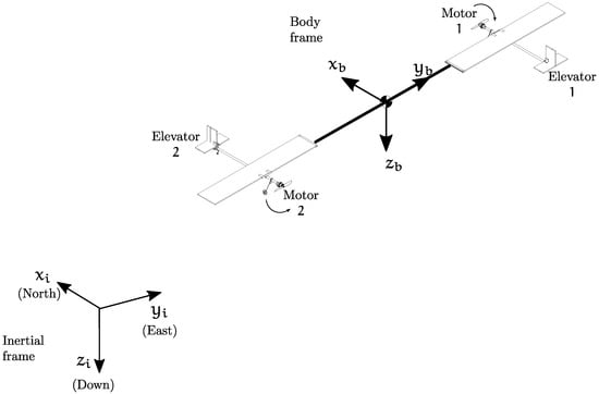
Figure 1.
Single rotor system represented in the three-dimensional space.
This prototype combines two of the most appreciated features in the UAV world, the aerodynamic efficiency of fixed-wing aircraft and the ability of helicopters to take off and land in confined areas.
The set of commands to drive this system is similar to that of a helicopter [12]. Its movements are referred to an inertial frame and to the body frame with origin in its center of mass. Increasing or decreasing the collective pitch of the wings will produce an increase or a reduction of the overall lift, which will generate a vertical movement. Tilting the rotation disk of the two planes generates a horizontal displacement. This is achieved by using the cyclic pitch control, which modifies pitch and roll of the aerial vehicle. The generation of cyclic pitch control will be explained later. Contrary to a helicopter, the yaw of the proposed prototype is not a control variable since the whole body of the aircraft remains turning. The movements will be labeled with an i sub-index or with a b subindex to denote that they are referred to the inertial or body frames respectively.
The Euler Lagrange approach [13] with external generalized force is employed to derive the equations of motion of the proposed set up, i.e.,
where is the generalized vector of moments and forces, is the Lagrangian defined as , is the kinetic energy, is the potential energy and is the generalized coordinates vector.
The main elements in the system are depicted in Figure 2. Where and are lift forces, and are drag forces, and and are trust forces, also the drag force on the rod is represented as and with similar characteristics to the drag force in each airplane.
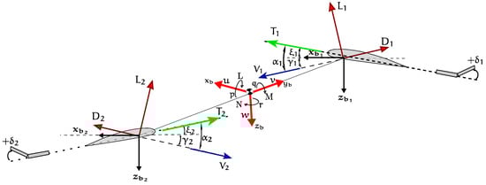
Figure 2.
Forces, moments and velocities acting on or upon the system.
In addition, the linear and angular velocity vectors are defined as
respectively, and
is the vector of moments of roll, pitch and yaw.
The generalized coordinates are selected as
where
are defined as the position vector and the vector of Euler’s angles, respectively.
3. Equations of the Euler Angles
The orientation of the vehicle is obtained using Euler’s angle approach which consists of consecutive rotations denoted by [14,15]. Then a particular orientation in the body frame is expressed in the inertial frame employing the following transformation
and the relation between Euler’s angles and angular velocities is defined as
which can be rewritten as
where
is the transformation matrix that relates these elements.
4. The Potential and Kinetic Energy
The system has translation and rotation movements with respect to the inertial axis system, and also produces kinetic and potential energy.
The total kinetic energy of the system is calculated as
where the first term corresponds to the translation kinetic energy and the second to the rotational kinetic energy and “I” being the inertia matrix of the system. If the vehicle is considered to be symmetrical the inertia matrix can be written as
and this inertial matrix must be represented with respect to the generalized coordinates system [16], so the following transformation is applied
therefore the rotational kinetic energy is rewritten as
in terms of the generalized coordinates.
The potential energy can be obtained as
where is the mass of the airplanes including that of the rod, g is the acceleration due to gravity and z is the height.
The Lagrangian is expressed as
which allows to find the Lagrange equations.
5. Forces and Moments Acting on the System
Euler-Lagrangre’s approach requires knowledge of the generalized vector forces , that is
where is a force vector represented in the inertial frame and is the vector of moments.
Firstly the forces in the body frame are obtained from Figure 2 as
where and are the forces due to aerodynamics and propulsion effects. The aerodynamics forces and propulsion forces are obtained as
where the angles of attack are defined as
also the lift forces (, ), drag forces (, , , ) and propulsion forces (, ) are defined as [17,18,19]:
where is called dynamic pressure, is the air density, is the air speed, S is the wing area or the rod area, n is the speed of the propeller revolutions, D is the propeller diameter, is the engine thrust coefficient and and are the lift and drag coefficients respectively.
The forces vector relative to the vehicle body is obtained as
where represents any force on the axis.
The force is obtained using the transformation given by (8) as follows
which is the force vector required by the Lagrange equations.
The vector of moments is obtained as
where M is any existing moments on the axis, , are moments on the axis and , are the moments on the axis associated to the drag force of the rod.
The forces and moments equations are simplified considering that the incidence of wind in the vehicle is negligible or not present, therefore Equations (23) and (24) become
i.e., the angle of attack is defined by the pitch of each profile, also the lateral forces on the vehicles are counteracted by each other, i.e., . Therefore the Equation (29) is written as
where
are the components of the force vector expressed in the inertial frame.
Due to of the high angular velocity in aircraft systems, they are modeled as a counterclockwise rotating disk [20] when viewed from above. Then the force Equations (34)–(36) with are rewritten as
taking into account that the propulsion forces in the engines are much larger than the drag forces in each vehicle, such that
are the forces considered in the x axis of the body.
6. Lagrange Equations of the System
Equations of motion are developed using the Lagrange approach outlined in the Equation (1). From this equation it is noted that the Lagrangian does not present cross terms between translation and rotational dynamics, so the Lagrangian is expressed as
therefore Equation (1) is rewritten as
these expressions represent the translational and rotational motions.
Firstly, the translation equations are obtained as
where
and expanding Equation (49) the following equations can be written
where Equations (51)–(53) are the equations corresponding to the translation motion.
Consequently, the rotational equations are obtained as
where the term is referred to as the Coriolis matrix that contains the gyroscopic and centrifugal terms associated with dependent on J [21].
Equation (55) can be expressed as
also considering that is obtained as (see Appendix A)
the following vector is defined
therefore expanding Equation (56) the following can be written
these equations represent the rotational dynamics.
7. Aerodynamic Equations of the Two Rotating Airplanes
Translational and rotational dynamics are obtained by expanding Equations (49) and (56). These equations are
expressed in terms of the generalized coordinates.
The group of equations associated with translational dynamics has elements that include the yaw variable and this evolves much faster than the other variables. The Equations (64)–(66) whose terms include sine and cosine functions of are then analyzed. Given the cyclic behavior of these components and considering that all other variables remain constant during a cycle, when they are integrated in a cycle from 0 to , the result is equal to zero. That is to say, the contribution of these components in the previous equations is zero and therefore the expressions of the translational accelerations can be simplified resulting in
and in order to simplify the rotational dynamics the following change of variable is proposed
substituting in the Equation (56) results in
8. Control Commands
Control commands applied to the system require a reference frame with respect to the pilot as shown in Figure 3, such that z is equivalent to and x is aligned with the front of the pilot. In this arrangement the frame with respect to the pilot coincides with the inertial frame but can be considered as a rotation on .
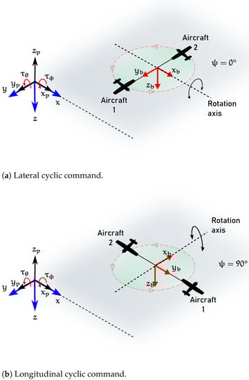
Figure 3.
Control commands.
The control signals , and are sent by the pilot. These signals are transformed into collective and cyclic control commands for the actuators.
Lateral Cyclic Command
The lateral cyclic command turns on when the vehicle reaches the positions as shown in Figure 3a. This control command produces roll motion and it can be obtained applying the equations
Longitudinal Cyclic Command
The longitudinal cyclic command occurs when the vehicle reaches the positions as shown in Figure 3b. This control command produces pitch motion and it can be obtained applying the equations
The rotation equations are written as
where the variables and have a sinusoidal behavior depending of yaw that produce displacement in x and y. As it was explained before, sinusoidal dynamics with respect to yaw are very fast therefore and only consider the effect of the sinusoidal dynamic at the moment when the maximum magnitude is produced during a cycle. This consideration implies that the resultant force produced by the two rotating airplanes point to the desired direction of the displacement where and define the magnitude of the tilt of the rotor disk formed by the system.
Alternatively, the equations describing the pitch and roll motions can be obtained as follows:
Consider that the two rotating airplanes are flying at a constant altitude and that the turning disk is horizontal. Suppose now that a sinusoidal signal is fed to the altitude or elevator control of each of the airplanes. The signal fed to the first aircraft is such that the elevator displacement is maximum when that aircraft passes over the north side of the turning disk and has its minimum value when it passes over the south side of the turning disk. A similar signal is fed to the second plane but out of phase .
In this way, the first plane increases its altitude as it passes from the north point to the east point and returns to its altitude when it reaches the south point. The second plane does something similar having the same height when passing from the south point to the north point but has a lower height when passing through the west point.
The result of this half-cycle is that the turning plane of the two planes has tilted slightly to the west, pivoting on the north-south axis. At the end of this half-cycle, the two rotating planes set up is ready to begin a second half-cycle in which it will tilt slightly more to the west. The magnitude of the tilt depends on the amplitude of the sinusoidal signal fed to the elevators. The direction of the axis in which the spinning disk pivots can be changed by changing the phase of the sinusoidal signal.
The lift forces generated on each aircraft are equal and expressed as a total thrust that acts perpendicular to the disc described by the two rotating aircraft. So the equations of the system are written as
9. Control Strategies
The dynamics of the altitude of the system of airplanes is associated to Equation (83), in order to stabilize the system at a desired height the following is proposed
where is a state feedback control such that
where and are positive constants and is the desired altitude [22].
The control law for the yaw angle given by
where is a positive constant and is the desired yaw velocity [23].
Substituting (86) into (83), the following is obtained
where the gains in are selected such that the altitude dynamics is faster than the horizontal dynamics.
Assuming that the desired altitude is reached and the following is obtained
The above equations represent equations represent the horizontal model where and are used to regulate the horizontal motion. In order to stabilize the system, the desired roll and pitch are selected as
where and are state feedback controllers such that
and , , and are positive constants.
Considering the required roll and pitch established before, the rotational dynamics is stabilized with
where , , and are positive constants.
When the desired control inputs (94) and (95) are satisfied the horizontal dynamic become
where the pair is asociated to the longitudinal motion and the pair is asociated to the lateral motion. The control process diagram is shown in Figure 4.
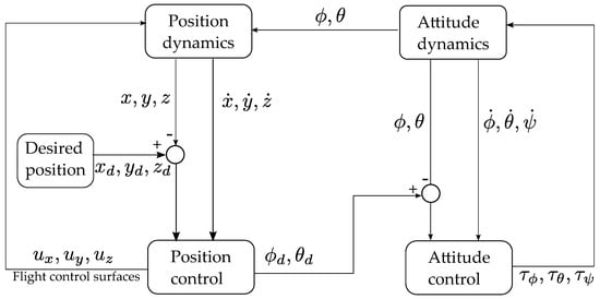
Figure 4.
Control process diagram.
10. Simulations Results
The following section presents the simulation results for the equations of the two rotating airplanes. The parameters used in the simulation are listed in the Table 1.

Table 1.
Simulation parameters.
Control gains were experimentally selected to satisfy the design requirements of attitude and position control, altitude control allows achieving the desired altitude without overshoot as shown in Figure 5. In addition, adjustment of the controller ensures that this dynamics is faster than the horizontal dynamics.
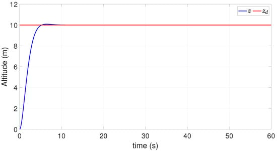
Figure 5.
Altitude response.
At the same time, yaw rate is regulated by the yaw control, so that a steady yaw rate is reached as shown in Figure 6.
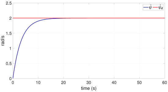
Figure 6.
Dynamics of yaw velocity.
Subsequently, the roll and pitch angles are used to regulate the horizontal dynamics. Then, the desired roll and pitch angles that stabilize the horizontal position are computed as shows Figure 7.
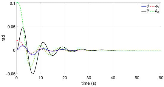
Figure 7.
Tracking of the desired angular trajectory.
As mentioned before, the pitch and yaw angles are related to the horizontal displacement, the position controllers inputs are shown in Figure 8 to reach the desired position.
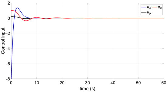
Figure 8.
Dynamics of the position controllers.
Orientation controllers behavior is shown in Figure 9, this dynamics allows the roll and pitch angles to be stabilized according to the desired angles calculated previously.
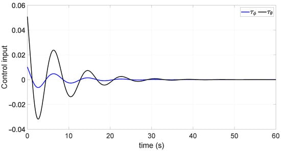
Figure 9.
Dynamics of attitude controls.
During the stabilization of the two rotating aircraft the generated total lift force is shown in Figure 10 which allows to carry out the regulation of the position.
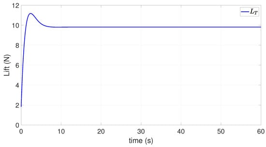
Figure 10.
Lift of the rotor disc.
In consequence, the aircraft system reaches the desired x-y position when the controls are implemented as shows Figure 11.
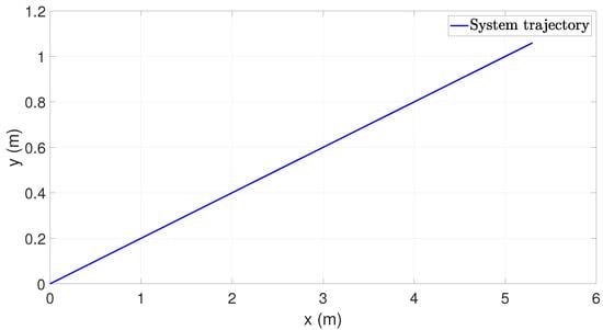
Figure 11.
System trajectory in the x-y plane.
11. Conclusions
This paper has clarified how a set of two attached rotating airplanes can be modeled and controlled. Besides the thrust of each of the airplanes, only the elevon is used for control purposes. Neither the ailerons nor the rudders are used as actuators. Once the kinetic and potential energies have been computed, the Euler-Lagrange approach is used to obtain the aerodynamical model of the prototype. Since the rotating speed is relatively high, some simplifications have been performed in the obtained model. Furthermore, since the two airplanes are assumed to be flying far apart from each other, we have neglected the induced flow which normally appears in classical helicopters.
In order to obtain pitch and roll moments of the prototype, we have created a virtual swashplate to emulate this central mechanism in helicopters. The virtual swhashplate was created by introducing a sinusoidal control on the airplanes’ elevators. The torque amplitude turned out to be proportional to the sinusoidal amplitude and the direction is determined by the phase of the introduced sinusoidal signal. A nonlinear control algorithm has then proposed to achieve a hover fligh at some particular position in space. The performance of the control strategy has been successfuly tested in numerical simulations.
Author Contributions
Conceptualization, investigation, writing—original draft preparation, J.A.B.-M.; Methodology, writing—review and editing, R.L.; Validation, supervision, A.O.-C. All authors have read and agreed to the published version of the manuscript.
Funding
This research was funded by CONACYT of Mexico through project 314879 “Laboratorio Nacional en Vehiculos Autonomos y Exoesqueletos LANAVEX”. The lead author was also supported by the UMI-LAFMIA CINVESTAV Mexico Preeminent Doctoral Program.
Institutional Review Board Statement
Not applicable.
Informed Consent Statement
Not applicable.
Conflicts of Interest
The authors declare no conflict of interest. The funders had no role in the design of the study; in the collection, analyses, or interpretation of data; in the writing of the manuscript, or in the decision to publish the results.
Appendix A. Inertia Matrix
The inertia matrix es defined as
with
and
expanding it follows
The inverse of the inertia matrix can be obtained by
with
References
- Sanchez-Rivera, L.M.; Lozano, R.; Arias-Montano, A. Development, Modeling and Control of a Dual Tilt-Wing UAV in Vertical Flight. Drones 2020, 4, 71. [Google Scholar] [CrossRef]
- Flores, G.; Escareño, J.; Lozano, R.; Salazar, S. Quad-Tilting Rotor Convertible MAV: Modeling and Real-Time Hover Flight Control. J. Intell. Robot. Syst. 2012, 65, 457–471. [Google Scholar] [CrossRef] [Green Version]
- Low, J.E.; Win, L.T.S.; Shaiful, D.S.B.; Tan, C.H.; Soh, G.S.; Foong, S. Design and dynamic analysis of a transformable hovering rotorcraft (thor). In Proceedings of the IEEE International Conference on Robotics and Automation (ICRA), Singapore, 29 May–3 June 2017. [Google Scholar]
- Escareño, J.; Salazar, S.; Lozano, R. Modelling and control of a convertible VTOL aircraft. In Proceedings of the IEEE Conference on Decision & Control, San Diego, CA, USA, 13–15 December 2006. [Google Scholar]
- Aktas, Y.O.; Ozdemir, U.; Dereli, Y.; Tarhan, A.F.; Cetin, A.; Vuruskan, A.; Yuksek, B.; Cengiz, H.; Basdemir, S.; Ucar, M.; et al. Rapid prototyping of a Fixed-Wing VTOL UAV for Design Testing. J. Intell. Robot. Syst. 2016, 84, 639–664. [Google Scholar] [CrossRef]
- Garcia, O.; Castillo, P.; Wong, K.C.; Lozano, R. Attitude stabilization with real-time experiments of a tail-sitter aircraft in horizontal flight. J. Intell. Robot. Syst. 2012, 65, 123–136. [Google Scholar] [CrossRef] [Green Version]
- Venkatesan, C. Fundamentals of Helicopter Dynamics; CRC Press: Boca Raton, FL, USA, 2014. [Google Scholar]
- Impulse, S. Solar Impulse Foundation: 1000 Profitable Solutions for the Environment. Available online: https://solarimpulse.com/ (accessed on 1 April 2021).
- Hernandez-Toral, J.L.; González-Hernández, I.; Lozano, R. Sun Tracking Technique Applied to a Solar Unmanned Aerial Vehicle. Drones 2019, 3, 51. [Google Scholar] [CrossRef] [Green Version]
- Ciotti, P. More with Less: Paul MacCready and the Dream of Efficient Flight; Encounter Books: San Francisco, CA, USA, 2002. [Google Scholar]
- VFS—Human Powered Helicopter. Available online: https://vtol.org/hph (accessed on 1 April 2021).
- Garcia, P.C.; Lozano, R.; Dzul, A.E. Modelling and Control of Mini-Flying Machines; Springer Science & Business Media: Berlin/Heidelberg, Germany, 2006. [Google Scholar]
- Goldstein, H.; Poole, C.P.; Safko, J.L. Classical Mechanics, 3rd ed.; Addison Wesley: San Francisco, CA, USA, 2002. [Google Scholar]
- Etkin, B.; Reid, L.D. Dynamics of Flight: Stability and Control, 3rd ed.; John Wiley & Sons, Inc.: Hoboken, NJ, USA, 1996. [Google Scholar]
- Cook, M.V. Flight Dynamics Principles: A Linear Systems Approach to Aircraft Stability and Control, 3rd ed.; Elsevier Ltd.: New York, NY, USA, 2013. [Google Scholar]
- Greenwood, D. Advanced Dynamics; Cambridge University Press: Cambridge, UK, 2006. [Google Scholar]
- Beard, R.W.; McLain, T.W. Small Unmanned Aircraft: Theory and Practice; Princeton University Press: Princeton, NJ, USA, 2012. [Google Scholar]
- Anderson, J.D., Jr. Fundamentals of Aerodynamics, 5th ed.; McGraw-Hill: New York, NY, USA, 2011. [Google Scholar]
- McCormick, B.W. Aerodynamics, Aeronautics, and Flight Mechanics, 2nd ed.; Wiley: New York, NY, USA, 1995. [Google Scholar]
- Fantoni, I.; Lozano, R. Non-linear control for underactuated mechanical systems. Appl. Mech. Rev. 2002, 55, B67–B68. [Google Scholar] [CrossRef]
- Lozano, R. Unmanned Aerial Vehicles: Embedded Control; John Wiley & Sons: Hoboken, NJ, USA, 2013. [Google Scholar]
- Cariño, J.; Lozano, R.; Bonilla Estrada, M. PVTOL control using feedback linearisation with dynamic extension. Int. J. Control 2019, 1–10. [Google Scholar] [CrossRef]
- Cabarbaye, A.; Lozano, R.; Bonilla Estrada, M. Adaptive quaternion control of a 3-DOF inertial stabilised platforms. Int. J. Control 2020, 93, 473–482. [Google Scholar] [CrossRef]
Publisher’s Note: MDPI stays neutral with regard to jurisdictional claims in published maps and institutional affiliations. |
© 2021 by the authors. Licensee MDPI, Basel, Switzerland. This article is an open access article distributed under the terms and conditions of the Creative Commons Attribution (CC BY) license (https://creativecommons.org/licenses/by/4.0/).