Navigation of Underwater Drones and Integration of Acoustic Sensing with Onboard Inertial Navigation System

Abstract

The navigation of autonomous underwater vehicles is a major scientific and technological challenge. The principal difficulty is the opacity of the water media for usual types of radiation except for the acoustic waves. Thus, an acoustic transducer (array) composed of an acoustic sonar is the only tool for external measurements of the AUV attitude and position. Another difficulty is the inconstancy of the speed of propagation of acoustic waves, which depends on the temperature, salinity, and pressure. For this reason, only the data fusion of the acoustic measurements with data from other onboard inertial navigation system sensors can provide the necessary estimation quality and robustness. This review presents common approaches to underwater navigation and also one novel method of velocity measurement. The latter is an analog of the well-known Optical Flow method but based on a sequence of sonar array measurements.

1. Introduction

Autonomous underwater vehicles (AUV) or “underwater drones” [1] constitute a significant class of robots that has many applications in various areas from commercial to military [2], including, e.g., marine archeology [3] and geoscience [4]. A number of possible applications are related to under-ice research in the Arctic seas [5,6]. Moreover, an explosive increase in AUV applications and market demand is predicted in the near future [7]. One of the most important issues is the navigation of AUVs, which is a major scientific and technological challenge. The principal well-known difficulty is the opacity of the water media for usual types of radiation except for acoustic waves. For example, computer vision, which is one of the major components in the autonomous vehicle data pipeline, is not applicable underwater since eyesight is much more limited (~5 m). Thus, for most of the practical needs, acoustic devices provide the easiest way to obtain information about the AUV localization and attitude [8]. One of the disadvantages of the acoustic tools is the inconstancy of the acoustic wave propagation speed, which depends on the temperature, salinity, and pressure [9] (Chapter 14). Thus, the construction of a robust navigation system requires the data fusion of the acoustic sensor measurements with information from other sensors in the onboard inertial navigation system (INS). Direct positioning is achieved by the measurement of the time of acoustic signal propagation from the vehicle to some objects with a known position. These methods are presented in Section 2 and Section 3. The direct positioning measurements can be effectively improved by adding the measurements of the vehicle velocity and then by fusing the result of the velocity integration with successive position measurements. One possible way to measure velocity is based on the Doppler effect, which manifests as the frequency shift proportional to the relative velocity. Special devices, such as acoustic Doppler current profilers (ADCP) and Doppler velocity logs (DVL), are widely used in underwater navigation. An example of the fusion of Doppler measurements with the data from the onboard navigation system and external positioning system will be given below in Section 4. Sonars or arrays of acoustic emitters–receivers provide more opportunities for underwater localization and navigation. Some of the applications and possible approaches based on their use will be given in Section 5 and Section 6. The measurements in underwater media generally lead to nonlinear observation equations, and most authors usually resort to various modifications of the Kalman Filter (KF), such as Extended Kalman Filter (EKF), Particle Filter, or Unscented KF. However, underwater measurements are indirect: instead of coordinates, they yield distances and/or bearing angles. For this reason, some of the mentioned methods have limited applicability, and more specialized approaches to estimation are necessary. Such approaches are presented in Section 7, where we describe the pseudo-measurement method and the conditional minimax filter. The former [10] has its origin in underwater applications, whereas the latter was successfully used in the control of aerial vehicles [11]. A transformation of these methods for estimation based on the distance to the seabed measured by sonar is presented in Section 7. Section 8 contains conclusions.

2. Baseline Positioning Systems

Underwater acoustic positioning systems are generally categorized into three broad classes [12], namely, long baseline (LBL), short baseline (SBL), and ultra-short baseline systems (USBL). The baseline approach implies measuring the range to several (three or more) spaced acoustic beacons with known coordinates and solving the corresponding system of equations, which connects the known beacons’ coordinates, measured distances, and AUV coordinates as unknown variables. In a detailed review [12], various realizations of this approach are presented, showing the necessity of different methods and various beacon placements depending on the real range of the AUV operation and the corresponding mission. Besides the beacons, an acoustic transducer array with known coordinates can be used. Transducers receive the acoustic signal, the source of which is the AUV itself (so this is the case when a threat to the AUV detection is irrelevant). In all baseline methods, the raw positioning data are resolved from the distances and angles between the sources and receivers of the acoustic signals (acoustic beacons, elements of the transducer arrays, AUV transponders). An imaginary line forming the sides of the reference triangle(s) is known as the “baseline”. The reference frame can be associated with the transponder array itself, a physical object (such as a dam, a ship, or a pier), or the Earth, and the AUV offset coordinates are calculated with respect to this frame. A comparison of different types of acoustic positioning arrangements is presented in [9] (Chapter 16).

2.1. Long Baseline Systems

The known LBL systems provide a rather high level of position accuracy—generally better than 1m. This level of accuracy is a standard for LBL, but in the case of very robust transponder positions, it can be improved up to $0.01$ m [13]. The transponders are typically mounted in the corners of the operational area. Usually, the positions of transponders are very stable if they are installed in the reference frame of the worksite itself (i.e., on the seabed). The wide transponder spacing results in excellent geometry for position computations. In most cases, the LBL system operates distantly from the sea surface to avoid producing additional noise. The usage of LBL covers various applications, such as underwater target localization [14], the fusion of INS and LBL [15], marine geodesy [16], and AUV self-localization [17]. More applications of LBL relate to Arctic research and navigation under the ice [5,6].

2.2. Ultra-Short Baseline Systems

Ultra-short baseline (USBL) systems (sometimes referred to as super-short baseline (SSBL) systems) [18] typically use relatively short (e.g., 230 mm across), tightly integrated transducer arrays. These arrays are usually mounted at the bottom end of a rack on the side or on the bottom of a surface vessel (SV). Unlike LBL and SBL systems, which determine the position by measuring multiple distances, the USBL transducer array is used to measure the target distance from the transducer rack (using the signal travel time) and the target direction (by measuring the phase shift of the response between the individual transducer array elements). The combination of distance and direction allows the calculation of the position of the tracked target relative to the surface ship. Additional sensors can be used, including GPS, a gyroscope, or a electronic compass, and a vertical reference unit can be used to compensate for the changes in position and orientation of the SV and its measuring rack. The advantage of USBL systems is that they do not require an array of transponders on the seabed. The disadvantage is that the positioning accuracy and reliability are inferior to those of LBL systems. This is because the low angular resolution of the USBL system results in a larger position error at a greater distance. In addition, each of the multiple sensors required for the position and orientation compensation introduces additional errors. Finally, since the underwater acoustic environment is non-homogeneous, it causes signal refractions and reflections, which have a greater impact on the positioning of the USBL than in the case of the LBL geometry. Interestingly, a strap-down inertial navigation system (SINS) with USBL can be effective means for underwater positioning [19]. USBL technology has been the primary choice in underwater positioning [20,21]. For a stand-alone SINS, its positioning error accumulates over time; nevertheless, the high-precision positioning technology needs the application of statistical methods for isolation of non-properly operating sensors [22]. In the work [23], it is shown that the high-precision phase difference information can be obtained based on the non-equidistant quaternary array and the phase difference acquisition mechanism.

2.3. Short Baseline Systems

Short baseline (SBL) systems use a baseline consisting of three or more individual sonar transducers that are connected by wire to a central control box. Accuracy depends on transducer spacing and mounting method. When wider spacing is employed, as when working from a large working barge or when operating from a dock or other fixed platform, the performance can be similar to LBL systems. When operating from a small boat, where transducer spacing is tight, accuracy is reduced. Similar to USBL systems, SBL systems are frequently mounted on boats and ships, but specialized modes of deployment are common too. For example, the Woods Hole Oceanographic Institution uses an SBL system to position the Jason deep-ocean ROV relative to its associated MEDEA depressor weight, with a reported accuracy of 9 cm [24].

2.4. GPS Intelligent Buoys

GPS intelligent buoy (GIB) systems can be regarded as inverted LBL devices, where the transducers are replaced by floating buoys, self-positioned through GPS [25,26]. The tracked position is calculated in real time at the surface from the time-of-arrival of the acoustic signals sent by the underwater device, and acquired by the buoys. Such configurations allow fast, calibration-free deployment with an accuracy similar to LBL systems. Contrary to LBL, SBL, or USBL systems, GIB systems use one-way acoustic signals from the emitter to the buoys, making it less sensitive to surface or wall reflections. One of the GIB systems presented by a French company, ACSA [26], can be used to track AUVs, torpedoes, or divers; it may be used also to localize airplanes’ black boxes and even mines. Another application is weapon testing and training, where GIB systems are used to determine the impact coordinates of inert or live weapons. An interesting approach to the optimization and modeling of GIB with the aid of neural networks is presented in [27]. In the paper [25], a general approach to GIB is presented, and a typical configuration of the positioning AUV system is given. The signal transmitted by the AUV at regular intervals is received by a set of buoys located in the vicinity of a surface vehicle. The coordinates of the underwater mobile can be calculated through the intersection of corresponding spheres. The advantages of this approach are the rather small period of installation and no need for calibration. It takes only one hour to install the GIB system, as reported in [25].

2.5. Comparison of Acoustical Positioning Methods

A detailed comparison of various acoustical positioning methods is presented in [9]; here, we summarize the information in Table 1.

Table 1. Acoustic positioning methods.

Method	Position of Beacons/Transponders	Accuracy	Note
LBL	Sea floor/surface	0.1–1 m	operation ranges limited (up to 5 km)
USBL	SV (surface vessel)	$>>$ 1 m	only limited by SV
SBL	SV/fixed platform	up to 0.1 m
GIBs	Sea surface	up to 1 m (as LBL)	easy installation

2.6. Positioning Systems Based on Absolute Velocity Measurements

Determining the position of an underwater vehicle in the absence of external measurements such as GPS requires the use of the capabilities of the onboard navigation system, which makes it possible to estimate the current speed and direction of movement in the global coordinate system [28]. However, the INS sensors are prone to drift, and huge integration errors might occur within a few minutes. Additional measurements can alleviate these issues and correct the INS errors. One of the most frequently used and, hence, the most important element of an underwater navigation system is the measurement of the speed. In modern devices, as a rule, Doppler speed meters are used, or their analogs, which allow the measurement of speed based on the evolution of the seabed image obtained using sonars or acoustic profilers. These navigation methods will be discussed below in Section 4, Section 5 and Section 6.

3. Various Approaches to Underwater GPS

In this section, we give a series of examples reporting the realization of acoustic GPS in various areas of application and different environments. As in the surface GPS, an underwater positioning system needs the creation of a network of nodes (acoustic buoys or transponders) with a known and very stable position. The unknown position of the vehicle is determined from the system of equations relating the vehicle’s unknown position and the times of the acoustic signal propagation between the AUV and the nodes. Various methods of AUV positioning and navigation are presented in the review [29].

3.1. Positioning Based on the Bio-Inspired Sensing

Recently, interesting bio-inspired methods of underwater positioning have emerged [30]. Even though the original optical methods are not directly applicable to underwater applications due to the extremely fast absorption of electromagnetic radiation in water, there are some features of the optical waves that remain, allowing for more or less reliable determination, which may be suitable for navigation purposes. Among them are color [31] and polarization [32]. It is difficult to judge the efficiency of this methodology in real navigation applications since the achieved accuracy of positioning is approximately 6 m per kilometer travelled [30]; however, the achievements in color and polarization registration are rather useful for zoological and bio-underwater research [33,34].

3.2. Positioning with GPS and Dual Acoustic Device with USBL and Forward-Looking Sonar Combination

An example of coordination of the ultra-short baseline (USBL) and forward-looking sonar (FLS) is given in [35]. This system overcomes the limitations of the existing underwater GPS positioning techniques, which can determine only the position of the target that carries an acoustic transponder device. The system also realizes the real-time positioning of random and unknown targets within any water area, indicates the latitude and longitude coordinates under the WGS84 (World Geodetic System 1984) coordinate system, and demonstrates very good mobility. The underwater GPS positioning system based on the dual acoustic device can extend GPS positioning to the underwater area by using an USBL and an FLS. The mother ship (MS) carries a differential GPS (DGPS) mobile station. The front end of the remotely operated underwater vehicle (ROV) is equipped with an FLS, and the USBL’s transceiver and the transponder are, respectively, installed on the bottom of the MS and the ROV. The USBL can coordinate with the DGPS and other auxiliary equipment to obtain the latitude and longitude coordinates under the WGS84 ellipsoidal coordinate system of the USBL’s transponder carried on the ROV. In addition, from the imaging of the target in the FLS and the relative position between the FLS and the USBL’s transponder, the variation in the coordinates of the target relative to the USBL’s transponder can be obtained. By superimposing these two results, the coordinates of the target in the WGS84 ellipsoidal coordinate system can be calculated.

3.3. Positioning Systems Based on Orthogonal Waveforms

Orthogonal waves are commonly applied in radar and sonar systems to solve multi-target detection problems. Currently, existing underwater acoustic positioning systems (UAPSs) can supply only a small number of users, mainly because there is no suitable signal for multi-target systems. In this work [36], the authors introduced orthogonal waveform theory to UAPSs and analyzed the performance of phase-coding signals according to different parameters. Then, based on the actual requirements, the authors designed a group of orthogonal waveform phase-coding signals using a genetic algorithm. They found that the signals designed had good correlation performance, excellent frequency resolution compared to tone signals, high Doppler tolerance, and were relatively unaffected by reverberation. Simulations conducted with different carrier frequencies showed that the proposed system was able to process more than 80 signals. The proposed signals also showed high time resolution and millisecond-level time delay estimation precision with 10 dB SNR (signal-to-noise ratio); further, the multi-path and aliasing performance of the proposed system were shown to meet real-world application requirements. Experimental results showed that the designed signals are suitable for UAPSs, with high positioning precision and continuous trajectory. Taken together, observations confirmed that the signals designed have highly favorable correlation performance and show attractive potential application in UAPSs.

3.4. Positioning System Based on GPS Surface Nodes and Encoded Acoustic Signals

In this work [37], an underwater positioning system based on beacons equipped with GPS and acoustic transducers has been characterized for different measurement errors related to environmental conditions and geometrical configurations. This system uses Kasami codes to improve the detection of the acoustic signals, obtaining a better estimation of the distances between the nodes, process gain against noise, and allowing for multiuser capabilities. Considering the measurement process of the system, any additional underwater vehicle in the environment only requires a different code to be identified and located. The vehicles would respond to the same code emitted by the ship and, taking advantage of the good cross-correlation properties of certain coding schemes, such as Kasami codes, no time guard protocol is needed, and the same measurement cycle and positioning algorithms can be used. This way, the number of underwater vehicles located by the positioning system could be easily increased at the expense of slightly increasing the computational time at the ship. The codes used by the underwater vehicles should be known by the beacons and the ship, so that they can distinguish from which one the received signal is coming in order to calculate their position.

3.5. Positioning with Long Baseline (LBL)

Conventional long baseline (LBL) acoustic navigation systems require multiple stationary transponders, i.e., fixed or moored on the sea floor [4]. With a maximum acoustic range of 5–10 km, fixed LBL networks can cover geographically limited mission areas. Moreover, the majority of commercially available LBL navigation systems available over the past 30 years were designed to use pulsed narrowband continuous waveforms. This design inherently limits to the system the navigation of one vehicle per interrogation–response acoustic cycle, which is usually scheduled through a time division multiple access (TDMA) schedule to avoid acoustic interference. Although this limitation is acceptable for single-vehicle deployments, it is less desirable for multi-vehicle deployments because the interrogation–response navigation update period increases linearly with the number of vehicles (thereby proportionally decreasing each vehicle overall navigation update rate). In practice, this limits tone-burst LBL navigation to networks of a few vehicles. Modern INS position error is on the order of 1 percent of the path length and, when properly calibrated and aided by a DVL, can approach the quality of 0.1 percent of the whole path length. LBL acoustic positioning uses travel times converted to ranges from two or more widely spaced (long baseline) stationary beacons (a net) to trilaterate the location of a moving receiver (vehicle) in two or three dimensions [8,38]. The beacons are typically stationary (fixed baseline) and moored to the sea floor with tethers. The beacons can also be held in fixed relative locations on a moving platform such as a ship (moving baseline). Their signals must be uniquely identifiable, which is typically accomplished through the assignment of unique coded pulses or frequencies to each beacon. The beacon locations must be determined during an initial offline survey. During operation, the receiver either actively interrogates (pings) the beacons acoustically and measures the round-trip travel time to each beacon or passively listens to the net being interrogated remotely or triggered on a synchronized time base. Travel times are converted to slant ranges that yield spherical constraints on vehicle position (active interrogation) or hyperbolic constraints (passive listening). Additional information, such as an independent estimate of the receiver’s depth, can also constrain the position fix. When the number of constraints matches the number of unknown positional degrees of freedom (exactly determined), a position fix can be attained geometrically. The overdetermined case is typically solved using least-squares methods. Although the basic premise of spherical and hyperbolic LBL navigation is straightforward, its implementation for deep-ocean navigation requires addressing beacon survey, sound velocity profile compensation, and various systematic and random noise sources.

3.6. Positioning with Long Baseline (LBL) under Ice

A few authors have discussed the design and performance of AUV navigation systems for polar latitudes [5]. They suggest an under-ice LBL positioning system based on a combination of ice-moored and sea-floor beacons [5,6].

Some authors report diver-towed underwater GPS receivers [39]. Even such reliable and low-cost solutions provide the GPS solution in limited size. Here, the main error source for exact positioning is the additional cable between the buoy and the diver. Such systems can achieve sub-meter accuracy.

3.7. Synchronous-Clock, One-Way-Travel-Time Acoustic Navigation

This approach demonstrates the development and deployment of a synchronous-clock acoustic navigation system suitable for the simultaneous navigation of multiple underwater vehicles [40,41]. Their navigation system is composed of an acoustic modem-based communication and navigation system that allows for onboard navigational data to be broadcast as a data packet by a source node and for all passively receiving nodes to be able to decode the data packet to obtain a one-way-travel-time (OWTT) pseudo-range measurement and navigational ephemeris data. The navigation method reported herein uses a surface ship, acting as a single moving reference beacon to a fleet of passively listening underwater vehicles. All vehicles within the acoustic range can concurrently measure their slant range to the reference beacon using the one-way-travel time measurement methodology and additionally receive transmission of the reference beacon position using the modem data packet. The advantages of this type of navigation system are that it can concurrently navigate multiple underwater vehicles within the vicinity of the surface ship and provide a bounded-error XY position measure that is commensurate with conventional moored long baseline (LBL) navigation systems (i.e., order of 1 m), but unlike LBL, it is not geographically restricted to a fixed-beacon network. The authors present results for two different field experiments using a two-node configuration consisting of a global positioning system-equipped surface ship acting as a global navigation aid to a Doppler-aided autonomous underwater vehicle. In each experiment, the vehicle position was independently corroborated by other standard navigation means. Results for a maximum likelihood sensor fusion framework are reported [42].

3.8. Comparison of Various Approaches to Underwater Positioning

We summarize the information on the GPS-like methods of underwater positioning in Table 2.

Table 2. Various underwater positioning methods.

Method	Additional Means	Accuracy	Operation Range	Multiple AUV
USBL + FLS	SV (surface vessel)	1.2 m	Close to SV	No
Orthogonal waveform		High		Yes
GPS surface beacon	Encoded signals	High	Close to beacon	Yes
LBL + OWTT	SV (surface vessel)	1 m (as LBL)	Close to SV	Yes

4. Doppler Effect-Based Acoustic Navigation

DVL [43], as well as ADCP [2], are the most important devices used for velocity tracking of the AUV [44]. As for DVL, it appeared relatively recently and consists of four emitters of periodical acoustic signals, directed in front of the vehicle, to determine the relative velocity between the vehicle and the seabed in four directions: forward, to the right, to the left, and backward. ADCP can measure the distribution of the water current velocity depending on the position of the measurement unit. Both these devices use the Doppler effect, which manifests in the change in the frequency of the emitted–reflected acoustic signal, which depends on the relative velocity of the vehicle and water. Usually, it is combined with the original location, the heading by the compass or gyroscope, and the acceleration sensor data. A set of sensors is combined (usually using the Kalman filter) [45], and the Janus matrix equation related to four channels of velocities measurement [46] is solved. The solution of these equations yields the estimate of the AUV absolute velocity, which is finally used in dead-reckoning to estimate the position of the vehicle. To minimize the possible errors, DVL needs calibration, which corrects the DVL position in the AUV coordinates frame and equalizes the coefficients of the four DVL measurements channels [47]. The main aim of the DVL is INS velocity assistance. Other additional auxiliary sources include bottom-track DVL and acoustic positioning with USBL. Data received from the AUV operation in real conditions showed the efficiency and sustainability of the proposed navigation system, its reliability, and robustness [48].

The usage of Doppler-based sensors in the INS [49] provides fruitful results in attitude measurement accuracy [50], which includes a small difference in scale factors in channels of order ${10}^{-3}$ and a small bias in the pitch, roll, and yaw channels. See Table 3, which presents the relative errors of measurement channels and orientation angles.

Table 3. Relative errors of measurement channels and errors of the orientation angles [50].

Scale factor	$1.0\times {10}^{-3}$	$3.3\times {10}^{-4}$	$3.3\times {10}^{-4}$
Pitch	$9.0\times {10}^{-2}$	$1.0\times {10}^{-2}$	$1.0\times {10}^{-2}$
Roll	$8.9\times {10}^{-2}$	$7.2\times {10}^{-4}$	$5.6\times {10}^{-4}$
Yaw	$8.1\times {10}^{-3}$	$4.2\times {10}^{-3}$	$3.8\times {10}^{-4}$

5. Navigation with the Aid of Position Estimation Algorithms Based on Acoustic Seabed Sensing and Angle Measurements

The onboard navigation systems of almost all AUVs are subject to uncontrolled bias, causing errors, which increase quite quickly compared to the time of the mission. Therefore, as a rule, it is necessary to correct the sensor readings. In unmanned aerial vehicles (UAVs), this correction can be carried out according to the readings of the satellite system or based on surface observations using video cameras. This requires special estimation methods given the bearing only observations and corresponding UAV control algorithms [51,52,53,54,55]. For underwater vehicles, these methods are not directly implementable due to the already mentioned limits of video recording. Moreover, as a rule, there are no detailed maps of the seabed relief, and the characteristic features—which, in the case of the seabed, could be rocks, the remains of shipwrecks, etc.—may also be absent. Hence, the underwater environment requires other types of INS measurement correction. One example of such correction is a depth map prepared in advance for the route of the planned mission. This map serves as a reference for the correction of the depth sensor readings and, accordingly, the position on the route [56]. A system of this type was designed for the AUV Autosub 6000. It allowed the estimation of drift in dead-reckoning navigation by comparing the observed bathymetric data in the multibeam echo sounder data with the reference map [57]. The reference map comprises single bathymetric line data, one swath width across, covering the mission work area. The paper discusses biases in common AUV navigation sensors and their impact on navigation on a map created during a mission using an underwater vehicle. To analyze navigation errors accumulated during the Autosub 6000 research mission and computational limitations for real-time applications, a filter was proposed based on the discussion in the paper.

5.1. Sonars

A significant improvement in the characteristics of acoustic rangefinder instruments and the possibility of combining them into arrays of emitters–receivers (sonars) opens up new perspectives in the use of acoustic methods for the positioning and navigation of autonomous underwater vehicles. The quality of the images formed by sonar allows the use of well-known processing techniques derived from visual optics. Nowadays, synthetic aperture sonars (SAS) and tomographic sonars are increasingly used in the acoustics of underwater vehicles [58,59].

A shallow-water SAS design requires an understanding of key systemic and environmental problems. The main features limiting SAS performance are the accuracy of micronavigation (the task of estimating the length of the acoustic path to allow focusing of the aperture), the effects of multipath propagation, and the target viewing angle changes. The accuracy of micronavigation has been successfully solved by a gyrostabilized antenna with a displaced phase center, which combines motion estimates based on data with external orientation sensors. The effects of multipath propagation in shallow water are effectively countered by a narrow vertical beam. The shadow blur caused by the change in the viewing angle is diminished by raising the center frequency to reduce the length of the SAS integration and at the same time supporting the desired resolution and by developing a system with a minimum glancing angle of around 6° to decrease the length of the shadow. These factors led to choosing a central frequency of 300 kHz and a multipath alleviation scheme with multiple vertical beams. Experimental results obtained with a sonar that includes these attributes allowed SAS images to be obtained with a resolution of 1.6–5 cm in the transverse cross-range, and the shadow contrast exceeded 5 dB at a range of up to 170 m at a depth of 20 m [60].

5.2. Design and Performance of Sonars

A comprehensive description of the sonar technology may be found in [61,62]. Sonars in AUV applications are used for underwater simultaneous localization and mapping (SLAM) [63], and in AUV navigation [29]. When an underwater object is insonified at many different viewing angles, the signals reflected from the object can be sampled in space and time by an array of sensors that can form a real or synthetic aperture. Backscattering signals contain spatial information that can be processed with inverse transformation methods to form an image of the two-dimensional spatial distribution of the acoustic reflectivity function of the object. The sector of the polar wavenumber spectrum, which is defined by data space or signal measurement space, quantifies the change with the aspect angle of the spatial frequency components that contribute to the backscattering signal. The radial sector extent is determined by the temporal bandwidth of the incident sonar pulse, and the angular extent of the sector is defined by the range of aspect angles over which the object is insonified. Similarly, the angular length of the sector is determined by the size of the aperture, which is formed by the positions of the sensor relative to the object. The described concept gives a generalized structure that combines sonar imaging techniques such as synthetic aperture sonar, image reconstruction from projections (reconstructive tomography), and side-scan sonar with a real aperture. The difference in these methods is directly due to the azimuthal angle subtended by the sensing array aperture. For a sonar with real aperture, this azimuthal angle is usually a fraction of a degree; for a sonar with a synthetic aperture with a strip map, it is several degrees; for a spotlight synthetic aperture sonar, it is tens of degrees; and for tomographic imaging sonar, it is 360°. Experimental results for a side-scan sonar with real aperture, a sonar with a synthetic aperture, and a tomographic sonar demonstrate that as the azimuthal extension of the angle formed by the sonar aperture increases, an acoustic image is developed from a single blurred point to an identifiable object.

6. Position Estimation with Seabed Sensing

The idea of this method was first suggested in [64]. Further mathematical developments were given in [65]. We emphasize that this method uses a well-known optical flow approach from UAV practice. An optical flow is a map of the local displacement rates of image points extracted from a sequence of video frames. Initially, these data were used to analyze the resolution of space and aero-imagery. However, it became clear that the assessment of the image shifts included information about the vehicle’s orientation and angular velocities, which made it possible to include these data in the system of angular and linear velocity sensors and incorporate them into the UAV control system. Of course, video filming in underwater vehicles is not possible in a way similar to the surface applications since the opacity of water media only allows objects to be observed within distances of less than 5 m. However, high-resolution sonar, which creates a distance map from the device to the seabed, can be a source of such “video information”. In our recent works [65], we proposed a distance-map-based method for the control and navigation of an AUV and provided comparison with traditional approaches. Thus far, as there are no explicit globally optimal solutions for the stochastic problems with nonlinear observations, we have considered the control and position estimation problems in the locally optimal formulation. The algorithm for position estimation is formulated on the dead-reckoning with speed evaluated from the “acoustic images” evolution. By “acoustic image” we refer to the seabed distances that are registered by the acoustic sonar. Moreover, we propose the filtering algorithms formulated on the AUV dynamic model and direction of arrival (DOA) measurements.

Here, we give a brief explanation of the position estimation algorithm proposed. Assume that an AUV has an array of acoustic sensors, which are aimed at the seabed at different angles $({\gamma }^i,{\theta }^j)$. At time instant $t_k$, acoustic sensors make an image: a set of measurements of the distance to the seabed ${\mathbf{L}}_k^{ij}=L({\mathbf{X}}_k,{\mathbf{u}}_k,{\gamma }^i,{\theta }^j)$, where ${\mathbf{X}}_k$ is the AUV position and ${\mathbf{u}}_k$ is its movement direction. Given the difference between the values of correspondent distance measurements ${\mathbf{L}}_k^{ij}$ and ${\mathbf{L}}_{k+1}^{ij}$ made at the consecutive time instants $t_{k+1}$ and $t_k$, we can obtain information about the shift in the AUV’s position $\Delta {\mathbf{X}}_{k+1}={\mathbf{X}}_{k+1}-{\mathbf{X}}_k$ and speed ${\mathbf{V}}_k$. This is achieved in a similar manner to the optical flow estimation by the Lucas–Kanade method [54], but in our case, an image is the set of acoustic measurements, and the role of pixel intensity is played by a single seabed distance.

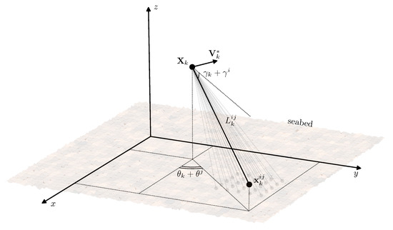
Let the AUV speed vector be defined by its absolute value $V_k=\parallel {\mathbf{V}}_k\parallel$ and two angles: ${\gamma }_k$, the angle between ${\mathbf{V}}_k$ and the horizontal plane $x0y$, and ${\theta }_k$, the angle between the projection of ${\mathbf{V}}_k$ on the horizontal plane $x0y$ and the axis $0x$. The acoustic beams are emitted by AUV sensors at the set of aiming angles $({\gamma }^i,{\theta }^j)$, $i,j=1,\dots ,M$. The absolute direction of the $(i,j)$ beam is given by the angles $({\gamma }_k+{\gamma }^i,{\theta }_k+{\theta }^j)$; see Figure 1.

Figure 1. Acoustic beam $(i,j)$ reaching the seabed surface at ${\mathbf{x}}_k^{ij}$.

At the time instant $t_k$ the $(i,j)$, beam reaches the sea floor at the point with coordinates ${\mathbf{x}}_k^{ij}={(x_k^{ij},y_k^{ij},z_k^{ij})}^T$, and ${\mathbf{e}}_k={(e_k^X,e_k^Y,e_k^Z)}^T$ is the beam direction:

$${\mathbf{x}}_k^{ij}={\mathbf{X}}_k+L_k^{ij}{\mathbf{e}}_k,$$

(1)

Let $\psi \left(\mathbf{x}\right)=0$ be the profile of the seabed, where $\psi (·)$ is some smooth function. If $\mathbf{x}$ is a function of $\mathbf{X}$, L, and $\mathbf{e}$, then

$$\mathbf{x}\left(t\right)=\mathbf{X}\left(t\right)+L\left(t\right)\mathbf{e}\left(t\right),$$

Now, we calculate the total derivative $\frac{d\psi \left(\mathbf{x}\right)}{dt}=\frac{d\psi \left(\mathbf{x}\right(\mathbf{X}\left(t\right),L\left(t\right),\mathbf{e}\left(t\right)\left)\right)}{dt}$.

Suppose that, at any seabed point reached by the acoustic beam, we know the partial derivatives of $\psi (·)$. Rewriting the total derivative in discrete time with substitution of the differentials with corresponding increments, we have the following equation:

$$\frac{\delta \psi }{\delta x}\left({\mathbf{x}}_k^{ij}\right)\Delta X_{k+1}+\frac{\delta \psi }{\delta y}\left({\mathbf{x}}_k^{ij}\right)\Delta Y_{k+1}+\frac{\delta \psi }{\delta z}\left({\mathbf{x}}_k^{ij}\right)\Delta Z_{k+1}=B_k^{ij},$$

(2)

with

$$\begin{array}{ccc}{B}_k^{ij}\hfill & =& -\frac{\delta \psi }{\delta x}\left({\mathbf{x}}_k^{ij}\right)\left(\Delta e_{k+1}^X{L}_k^{ij}+e_k^X\Delta L_{k+1}^{ij}\right)\hfill \\ \hfill & & -\frac{\delta \psi }{\delta y}\left({\mathbf{x}}_k^{ij}\right)\left(\Delta e_{k+1}^Y{L}_k^{ij}+e_k^Y\Delta L_{k+1}^{ij}\right)\hfill \\ \hfill & & -\frac{\delta \psi }{\delta z}\left({\mathbf{x}}_k^{ij}\right)\left(\Delta e_{k+1}^Z{L}_k^{ij}+e_k^Z\Delta L_{k+1}^{ij}\right).\hfill \end{array}$$

(3)

The unknowns $\Delta X_{k+1}$, $\Delta Y_{k+1}$, $\Delta Z_{k+1}$ can be estimated with the method of least-squares:

$$\Delta {\widehat{\mathbf{X}}}_{k+1}=\underset{\Delta {\mathbf{X}}_{k+1}}{argmin}\sum _{i,j=1}^M{\left(\frac{\delta \psi }{\delta x}\left({\mathbf{x}}_k^{ij}\right)\Delta X_{k+1}+\frac{\delta \psi }{\delta y}\left({\mathbf{x}}_k^{ij}\right)\Delta Y_{k+1}+\frac{\delta \psi }{\delta z}\left({\mathbf{x}}_k^{ij}\right)\Delta Z_{k+1}-B_k^{ij}\right)}^2$$

(4)

Rewriting Equation (2) in vector form with respect to the aiming angles set $({\gamma }^i,{\theta }^j)$, $i,j=1,\dots ,M$

$${\mathbf{A}}_k\Delta {\mathbf{X}}_{k+1}={\mathbf{B}}_k,$$

where ${\mathbf{A}}_k$ and ${\mathbf{B}}_k$ are formed by vertically stacked row-vectors and values which correspond to the individual observations:

$${\mathbf{A}}_k=\left(\begin{array}{ccc}\frac{\delta \psi }{\delta x}\left({\mathbf{x}}_k^{11}\right)& \frac{\delta \psi }{\delta x}\left({\mathbf{x}}_k^{11}\right)& \frac{\delta \psi }{\delta x}\left({\mathbf{x}}_k^{11}\right)\\ ⋮& ⋮& ⋮\\ \frac{\delta \psi }{\delta x}\left({\mathbf{x}}_k^{1M}\right)& \frac{\delta \psi }{\delta x}\left({\mathbf{x}}_k^{1M}\right)& \frac{\delta \psi }{\delta x}\left({\mathbf{x}}_k^{1M}\right)\\ ⋮& ⋮& ⋮\\ \frac{\delta \psi }{\delta x}\left({\mathbf{x}}_k^{MM}\right)& \frac{\delta \psi }{\delta x}\left({\mathbf{x}}_k^{MM}\right)& \frac{\delta \psi }{\delta x}\left({\mathbf{x}}_k^{MM}\right)\end{array}\right),{\mathbf{B}}_k=\left(\begin{array}{c}{B}_k^{11}\\ ⋮\\ B_k^{1M}\\ ⋮\\ B_k^{MM}\end{array}\right).$$

(5)

Then, the least-squares optimization problem (4) solution can be obtained in the common form:

$$\Delta {\widehat{\mathbf{X}}}_{k+1}={\left[{\mathbf{A}}_k^T{\mathbf{A}}_k\right]}^{-1}{\mathbf{A}}_k^T{\mathbf{B}}_k.$$

(6)

and the dead-reckoning estimate of the AUV’s position is

$${\widehat{\mathbf{X}}}_{k+1}={\widehat{\mathbf{X}}}_k+\Delta {\widehat{\mathbf{X}}}_{k+1}.$$

(7)

Here, we summarize the algorithm for the proposed AUV position estimation method with acoustic seabed sensing:

• at time instant $t_{k+1}$, measure the seabed distances $L_{k+1}^{ij}$ using the acoustic sensors $i,j=1,\dots ,M$ and obtain the increments $\Delta L_{k+1}^{ij}=L_{k+1}^{ij}-L_k^{ij}$;
• considering the direction angles’ values on the current step $({\gamma }_{k+1},{\theta }_{k+1})$ and the previous one $({\gamma }_k,{\theta }_k)$, calculate the increments ${(\Delta e_{k+1}^X,\Delta e_{k+1}^Y,\Delta e_{k+1}^Z)}^T$ using ${\mathbf{e}}_k={(e_k^X,e_k^Y,e_k^Z)}^T=(cos({\gamma }_k+{\gamma }^i)cos({\theta }_k+{\theta }^j)$, $cos({\gamma }_k+{\gamma }^i)sin({\theta }_k+{\theta }^j)$, $sin({\gamma }_k+{\gamma }^i){)}^T$;
• evaluate the slope estimates $\widehat{\frac{\delta \psi }{\delta x}}\left({\mathbf{x}}_k^{ij}\right)$, $\widehat{\frac{\delta \psi }{\delta y}}\left({\mathbf{x}}_k^{ij}\right)$, $\widehat{\frac{\delta \psi }{\delta z}}\left({\mathbf{x}}_k^{ij}\right)$;
• using (3) and (5), obtain the ${\mathbf{A}}_k$ matrix and the ${\mathbf{B}}_k$ vector;
• obtain the AUV position shift estimate $\Delta {\widehat{\mathbf{X}}}_{k+1}$ with (6) and calculate the position estimate ${\widehat{\mathbf{X}}}_{k+1}$ using (7).

7. DOA Measurement Position Estimation

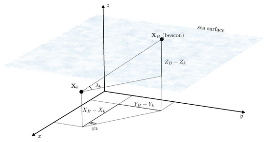
Here, we propose algorithms for position estimation formulated on the UAV linear dynamic model [65] and the external bearing-only measurements given by a passive acoustic DOA estimation device [61]. Consider that we know the coordinates of the pre-deployed stationary acoustic beacon ${\mathbf{X}}_B={(X_B,Y_B,Z_B)}^T$. We assume that the bearing vector (Figure 2) can be observed at any time instant $t_k$:

$${\mathbf{Y}}_k=\left(\begin{array}{c}tan{\phi }_k\\ tan{\lambda }_k\end{array}\right),\begin{array}{c}{\displaystyle tan{\phi }_k=\frac{Y_B-Y_k}{X_B-X_k}+{\epsilon }_k^{\phi },}\hfill \\ {\displaystyle tan{\lambda }_k=\frac{(Z_B-Z_k)cos{\phi }_k}{X_B-X_k}+{\epsilon }_k^{\lambda },}\hfill \end{array}$$

(8)

where ${\mathbf{E}}_k={({\epsilon }_k^{\phi },{\epsilon }_k^{\lambda })}^T\sim P^{{\mathbf{E}}_k}\in \mathcal{P}(\mathbf{0},{\mathbf{S}}^{\epsilon })$ is the i.i.d. random vector sequence independent of ${\mathbf{W}}_k$ and ${\mathbf{X}}_0$. Assume that, as in the case of the noise in the state equation, the exact distribution of these vectors is unknown [65].

Figure 2. Bearing to the point (beacon) with known coordinates ${\mathbf{X}}_B$.

The system of the vehicle motion and observations (8) can be written in the general vector form:

$$\begin{array}{c}{\mathbf{X}}_{k+1}={\Phi }_k({\mathbf{X}}_k,{\mathbf{u}}_k)+{\mathbf{W}}_k,\hfill \\ {\mathbf{Y}}_k={\Psi }_k\left({\mathbf{X}}_k\right)+{\mathbf{E}}_k.\hfill \end{array}$$

(9)

The EKF is the most direct approach to filtering in a nonlinear system; however, some disadvantages of EKF are well known. For example, a large deviation in initial estimation usually leads to the fast divergence of estimates; moreover, this issue cannot be solved even by such modern KF modifications as particle filter or UKF. For this reason, for a particular problem, it can be more beneficial to use some specific features of the setting, and with bearing-only observations, the pseudo-measurement and conditionally minimax nonlinear filter (CMNF), which exploit such features, turn out to yield stable estimates. Below, we demonstrate both of these approaches in the context of application to AUV navigation based on the evolution of the sonar distance measuring map.

We propose new approaches that, in some cases, allow us to obtain a better quality of estimation than direct linearization of the system. First, we give the transformation of the observation Equation (8), which allows us to reduce the original problem to a form in which the optimal filtering solution is also available in the form of a Kalman filter. Second, we give a statement and solution of the CMNF problem for the initial nonlinear model (9). This specific filtering approach allows data fusion of DOA measurements and the dead-reckoning navigation system based on the acoustic distance measurements of the seabed from Section 6.

7.1. Pseudo-Measurement Filter

We rewrite the observations (8):

$$\begin{array}{c}{\displaystyle (X_B-X_k)sin{\phi }_k=(Y_B-Y_k)cos{\phi }_k+{\epsilon }_k^{\phi }(X_B-X_k)cos{\phi }_k,}\hfill \\ {\displaystyle (X_B-X_k)sin{\lambda }_k=(Z_B-Z_k)cos{\phi }_{k}cos{\lambda }_k+{\epsilon }_k^{\lambda }(X_B-X_k)cos{\lambda }_k,}\hfill \end{array}$$

and then, at the left-hand side, we gather all the known or measured values:

$$\begin{array}{c}{\displaystyle X_{B}sin{\phi }_k-Y_{B}cos{\phi }_k=X_{k}sin{\phi }_k-Y_{k}cos{\phi }_k+{\epsilon }_k^{\phi }(X_B-X_k)cos{\phi }_k,}\hfill \\ {\displaystyle X_{B}sin{\lambda }_k-Z_{B}cos{\phi }_{k}cos{\lambda }_k=X_{k}sin{\lambda }_k-Z_{k}cos{\phi }_{k}cos{\lambda }_k+{\epsilon }_k^{\lambda }(X_B-X_k)cos{\lambda }_k.}\hfill \end{array}$$

(10)

The right-hand side is linear with respect to the system state ${\mathbf{X}}_k={(X_k,Y_k,Z_k)}^T$. At the same time, it carries the additive noise with state-dependent covariance. Let us now introduce the pseudo-measurement vector:

$${\mathbf{Y}}_k^{\prime }=\left(\begin{array}{c}{\displaystyle X_{B}sin{\phi }_k-Y_{B}cos{\phi }_k}\hfill \\ {\displaystyle X_{B}sin{\lambda }_k-Z_{B}cos{\phi }_{k}cos{\lambda }_k}\hfill \end{array}\right)$$

and rewrite (10) in vector form:

$${\mathbf{Y}}_k^{\prime }={\mathsf{\Psi }}_k^1{\mathbf{X}}_k+{\mathsf{\Psi }}_k^2{\mathbf{E}}_k,$$

(11)

where

$$\begin{array}{c}{\mathsf{\Psi }}_k^1={\mathsf{\Psi }}_k^1\left({\mathbf{Y}}_k\right)=\left(\begin{array}{ccc}{\displaystyle sin{\phi }_k}& -cos{\phi }_k& 0\\ {\displaystyle sin{\lambda }_k}& 0& -cos{\phi }_{k}cos{\lambda }_k\end{array}\right)\\ {\mathsf{\Psi }}_k^2={\mathsf{\Psi }}_k^2({\mathbf{X}}_k,{\mathbf{Y}}_k)=\left(\begin{array}{cc}{\displaystyle (X_B-X_k)cos{\phi }_k}& 0\\ {\displaystyle 0}& (X_B-X_k)cos{\lambda }_k\end{array}\right)\end{array}$$

The pseudo-measurement method is based on the idea that, in the case of linear observations and system dynamics, an estimate gathered with a linear Kalman filter will be linear-optimal [66]. Assuming that the noise ${\mathsf{\Psi }}_k^2{\mathbf{E}}_k$ covariance is state-dependent, we can evaluate or replace the estimate by an upper bound. In [51], we proposed a filtering algorithm based on the pseudo-measurements. Its recurrence relations were obtained using the unbiasedness of the previous step of estimate assumption. We can apply these relations to the problem at hand:

$$\begin{array}{c}{\tilde{\mathbf{X}}}_k={\mathsf{\Phi }}_{k-1}({\widehat{\mathbf{X}}}_{k-1},{\mathbf{u}}_{k-1}),\hfill \\ {\tilde{\mathbf{K}}}_k={\widehat{\mathbf{K}}}_{k-1}+{\mathbf{S}}^W,\hfill \\ {\overline{\mathbf{K}}}_k={\tilde{\mathbf{K}}}_k{{\mathsf{\Psi }}_k^1}^T\left(Y_k\right){\left({\mathsf{\Psi }}_k^1\left(Y_k\right){\tilde{\mathbf{K}}}_k{{\mathsf{\Psi }}_k^1}^T\left(Y_k\right)+{\mathsf{\Psi }}_k^2({\tilde{\mathbf{X}}}_k,{\mathbf{Y}}_k){\mathbf{S}}^{\epsilon }{{\mathsf{\Psi }}_k^2}^T({\tilde{\mathbf{X}}}_k,{\mathbf{Y}}_k)\right)}^{+}\hfill \\ {\widehat{\mathbf{X}}}_k={\tilde{\mathbf{X}}}_k+{\overline{\mathbf{K}}}_k\left({\mathbf{Y}}_k^{\prime }-{\mathsf{\Psi }}_k^1{\mathbf{X}}_k\right)\hfill \\ {\widehat{\mathbf{K}}}_k=(\mathbf{I}-{\overline{\mathbf{K}}}_k{\mathsf{\Psi }}_k^1\left(Y_k\right)){\tilde{\mathbf{K}}}_k\hfill \end{array}$$

(12)

The above filter has a common Kalman structure: upon an update of bearing measurements, all items are calculated recurrently. However, differing from the standard case, we cannot solve the Riccati equation a priori since it includes estimate-dependent terms and current measurement values.

7.2. Conditionally Minimax Nonlinear Filter (CMNF)

Suppose that functions ${\Phi }_k(·,·)$, ${\Psi }_k(·)$ and the feedback control ${\mathbf{u}}_k={\mathbf{u}}_k({\mathbf{Y}}_0,\dots ,{\mathbf{Y}}_k)$ such that the state ${\mathbf{X}}_k$ and observation ${\mathbf{Y}}_k$ first and second moments are finite. Bring in two functions sets: base prediction ${\alpha }_k(x,u)$ and base correction ${\beta }_k(x,y)$. Now, the CMNF estimate will be given by the subsequent recurrent relations:

$$\begin{array}{cc}{\tilde{\mathbf{X}}}_k=F_k{\alpha }_k({\widehat{\mathbf{X}}}_{k-1},{\mathbf{u}}_{k-1})+f_k,\hfill & F_k=cov({\mathbf{X}}_k,{\alpha }_k({\widehat{\mathbf{X}}}_{k-1},{\mathbf{u}}_{k-1}))\times \hfill \\ & {cov}^{+}({\alpha }_k({\widehat{\mathbf{X}}}_{k-1},{\mathbf{u}}_{k-1}),{\alpha }_k({\widehat{\mathbf{X}}}_{k-1},{\mathbf{u}}_{k-1})),\hfill \\ \hfill & f_k=\mathbf{E}\left\{{\mathbf{X}}_k\right\}-F_k\mathbf{E}\left\{{\alpha }_k({\widehat{\mathbf{X}}}_{k-1},{\mathbf{u}}_{k-1})\right\}\hfill \\ {\widehat{\mathbf{X}}}_k={\tilde{\mathbf{X}}}_k+H_k{\beta }_k({\tilde{\mathbf{X}}}_k,{\mathbf{Y}}_k)+h_k,\hfill & H_k=cov({\mathbf{X}}_k-{\tilde{\mathbf{X}}}_k,{\beta }_k({\tilde{\mathbf{X}}}_k,{\mathbf{Y}}_k))\times \hfill \\ \hfill & {cov}^{+}({\beta }_k({\tilde{\mathbf{X}}}_k,{\mathbf{Y}}_k),{\beta }_k({\tilde{\mathbf{X}}}_k,{\mathbf{Y}}_k)),\hfill \\ \hfill & h_k=-H_k\mathbf{E}{\beta }_k({\tilde{\mathbf{X}}}_k,{\mathbf{Y}}_k),\hfill \end{array}$$

(13)

Here, we have $cov(\mathbf{x},\mathbf{y}),$ which is the two random vectors $\mathbf{x}$, $\mathbf{y}$ covariance matrix; ${\mathbf{A}}^{+}$ is the matrix pseudo-inversion, and ${\widehat{\mathbf{X}}}_0={\mathbf{m}}_0$.

If, for all the random arguments in (13), the functions ${\alpha }_k(·,·)$ and ${\beta }_k(·,·)$ have first- and second-order moments, then there exists the CMNF estimate. Its minimax property has the following form. If the CMNF estimate at the time instant $t_{k-1}$ is ${\widehat{\mathbf{X}}}_{k-1}$, then the linear functions ${\mathcal{F}}_k^{*}\left(\xi \right)=F_k\xi +f_k$, ${\mathcal{H}}_k^{*}\left(\zeta \right)=H_k\zeta +h_k$ defined by (13) give the solution for the following problem of minimax optimization:

$$\begin{array}{c}{\displaystyle {\mathcal{F}}_k^{*}(·)=\underset{{\mathcal{F}}_k(·)}{argmin}\underset{P_k^{\prime }}{max}\mathbf{E}\parallel {\mathcal{F}}_k\left({\alpha }_k({\widehat{\mathbf{X}}}_{k-1},{\mathbf{u}}_{k-1})\right)-{\mathbf{X}}_k{\parallel }^2,}\hfill \\ {\displaystyle {\mathcal{H}}_k^{*}(·)=\underset{{\mathcal{H}}_k(·)}{argmin}\underset{P_k^{″}}{max}\mathbf{E}\parallel {\mathcal{H}}_k\left({\beta }_k({\tilde{\mathbf{X}}}_k,{\mathbf{Y}}_k)\right)-({\mathbf{X}}_k-{\tilde{\mathbf{X}}}_k){\parallel }^2,}\hfill \end{array}$$

(14)

where $P_k^{\prime }\in \mathcal{P}(\mathbf{E}{\mathcal{Z}}_k^{\prime },cov({\mathcal{Z}}_k^{\prime },{\mathcal{Z}}_k^{\prime }))$ is the set of all possible distributions of the compound vector ${\mathcal{Z}}_k^{\prime }={({\mathbf{X}}_k,{\alpha }_k({\widehat{\mathbf{X}}}_{k-1},{\mathbf{u}}_{k-1}))}^T$ and $P_k^{″}\in \mathcal{P}(\mathbf{E}{\mathcal{Z}}_k^{″},cov({\mathcal{Z}}_k^{″},{\mathcal{Z}}_k^{″}))$ is the set of all possible distributions of the compound vector ${\mathcal{Z}}_k^{″}={({\mathbf{X}}_k-{\tilde{\mathbf{X}}}_k,{\beta }_k({\tilde{\mathbf{X}}}_k,{\mathbf{Y}}_k))}^T$.

A detailed description of the CMNF approach to estimating the state of nonlinear stochastic systems, including a thorough justification of the fact that (13) is the solution to the problem (14) and the existence of solution conditions (14), can be found in [67]. The following papers are devoted to the further application of the concept along with a comparative numerical study [68,69,70]. Full detailed research is given in [65].

The CMNF estimate (13) being a minimax problem (14) solution indicates that, at each time $t_k$, it gives the minimum for the worst case (with respect to the a priori uncertainty in the distributions $P_k^{\prime }$ and $P_k^{″}$) of the mean square error of the prediction ${\tilde{\mathbf{X}}}_k$ and the correction ${\widehat{\mathbf{X}}}_k$. It should be noted that both ${\tilde{\mathbf{X}}}_k$ and ${\widehat{\mathbf{X}}}_k$ are unbiased estimates of ${\mathbf{X}}_k$, and that these estimates’ quality is known a priori:

$$\begin{array}{c}{\displaystyle cov({\mathbf{X}}_k-{\tilde{\mathbf{X}}}_k,{\mathbf{X}}_k-{\tilde{\mathbf{X}}}_k)=cov({\mathbf{X}}_k,{\mathbf{X}}_k)-F_{k}cov({\alpha }_k({\widehat{\mathbf{X}}}_{k-1},{\mathbf{u}}_{k-1}),{\mathbf{X}}_k),}\hfill \\ {\displaystyle cov({\mathbf{X}}_k-{\widehat{\mathbf{X}}}_k,{\mathbf{X}}_k-{\widehat{\mathbf{X}}}_k)=cov({\mathbf{X}}_k-{\tilde{\mathbf{X}}}_k,{\mathbf{X}}_k-{\tilde{\mathbf{X}}}_k)-H_{k}cov({\beta }_k({\tilde{\mathbf{X}}}_k,{\mathbf{Y}}_k),{\mathbf{X}}_k-{\tilde{\mathbf{X}}}_k).}\hfill \end{array}$$

Although Equation (7) completely defines the CMNF filter for a nonlinear stochastic system in quite a general form (9), which actually spans the AUV navigation problem at hand, there are two more questions to be considered in order to clear all the sides of the practical CMNF application: the functions $\alpha (x,u)$, $\beta (x,y)$, and the covariance calculation in (13).

The selection of base prediction and correction functions $\alpha (x,u)$, $\beta (x,y)$ depends on the model, and it represents specific features of the nonlinear functions ${\Phi }_k(·,·)$, ${\Psi }_k(·)$. The general option nonetheless is the prediction “by virtue of the system” and the correction in the form of residual, which, in the case of the linear dynamical system and observations model (8) with $\mathbf{E}\left\{{\mathbf{W}}_k\right\}=0$ and $\mathbf{E}\left\{{\mathbf{E}}_k\right\}=0$, has the following form:

$$\begin{array}{c}{\alpha }_{k+1}({\widehat{\mathbf{X}}}_k,{\mathbf{u}}_k)={\Phi }_k({\widehat{\mathbf{X}}}_k,{\mathbf{u}}_k)={\widehat{\mathbf{X}}}_k+{\mathbf{V}}_k\left({\mathbf{u}}_k\right)\Delta t,\hfill \\ {\beta }_k({\tilde{\mathbf{X}}}_k,{\mathbf{Y}}_k)={\mathbf{Y}}_k-{\Psi }_k\left({\tilde{\mathbf{X}}}_k\right).\hfill \end{array}$$

(15)

In contrast to pseudo-measurement filtering and EKF, the CMNF approach offer an easy means of INS and external measurement data fusion. The base prediction function ${\alpha }_{k+1}({\widehat{\mathbf{X}}}_k,{\mathbf{u}}_k)$ can be chosen in the form of the estimate from the internal navigation system (7). Finally, the CMNF estimate, obtained with the data fusion from the dead-reckoning seabed sensing and external bearing-only measurements, is given by (13) with structure functions

$$\begin{array}{c}{\alpha }_{k+1}({\widehat{\mathbf{X}}}_k,{\mathbf{u}}_k)={\widehat{\mathbf{X}}}_k+\Delta {\widehat{\mathbf{X}}}_{k+1},\hfill \\ {\beta }_k({\tilde{\mathbf{X}}}_k,{\mathbf{Y}}_k)={\mathbf{Y}}_k-\left(\begin{array}{c}{\displaystyle \frac{Y_B-{\tilde{Y}}_k}{X_B-{\tilde{X}}_k}}\\ {\displaystyle \frac{Z_B-{\tilde{Z}}_k}{\sqrt{{(X_B-{\tilde{X}}_k)}^2+{(Y_B-{\tilde{Y}}_k)}^2}}}\end{array}\right),\hfill \end{array}$$

(16)

here, $\Delta {\widehat{\mathbf{X}}}_{k+1}$ is the shift defined by (6) and the corresponding algorithm described in Section 6.

There is only one question left: the covariance matrices that are necessary to calculate the linear estimator coefficients in (13). The general CMNF approach implies that, instead of real covariances, their estimates obtained using Monte Carlo sampling are used.

The efficiency of the proposed algorithms, namely the conditional minimax nonlinear filter and the pseudo-measurement filter, was experimentally evaluated. Details of the modeling of pesudomeasurement and conditionally minimax filters are given in [65], and the software code for modeling can be found in [71]. The tests show that in an ideal situation with good initial accuracy and observation conditions close to those for a linear system (when the beacons are far away), the gain in the quality of the estimate and, consequently, in the control characteristics for pseudo-measurement filter and the CMNF is inessential compared to the standard extended Kalman filter. However, the proposed filtering algorithms can demonstrate better qualities in less auspicious conditions; for example, when one of the beacons is near the starting point of the path, the EKF diverges, but the proposed filters remain stable. One more result is that linear filters (pseudo-measurements and EKF) are very sensitive to the description of a dynamic model, and an inaccurate definition or estimation of parameters also leads to divergence, and only the CMNF filter allowed us to achieve a reasonable estimate/control performance.

8. Conclusions

The paper presents the principal directions in the area of underwater navigation for AUVs. Since the most accessible means of external sensing is acoustic, we present various approaches, which are used in combination with acoustic means with INS and correct biases inherent to its functioning. In addition to the approaches well-presented in the literature and practice of underwater research, we suggest a method that is an analog of the optical flow known in the video navigation of the unmanned aerial vehicles. In this method, the role of the video camera is played by sonar, and the image is formed as a set of seabed distances. Of course, the methods inherent to the optical flow need further improvement and cannot be directly applied, but this approach has already been developed in our recent work.

References

- Ehlers, F. (Ed.) Autonomous Underwater Vehicles: Design and Practice; Radar, Sonar & Navigation, Institution of Engineering and Technology: Stevenage, UK, 2020. [Google Scholar] [CrossRef] [Scilit]
- Gelin, C. A High-Rate Virtual Instrumentof Marine Vehicle Motions for Underwater Navigation and Ocean Remote Sensing; Springer Series on Naval Architecture, Marine Engineering, Shipbuilding and Shipping; Springer: Berlin/Heidelberg, Germany, 2013. [Google Scholar] [CrossRef] [Scilit]
- Foley, B.; Mindell, D. Precision Survey and Archaeological Methodology in Deep Water. ENALIA Annu. J. Hell. Inst. Mar. Archaeol. 2002, VI, 49–56. [Google Scholar]
- Wynn, R.B.; Huvenne, V.A.; Le Bas, T.P.; Murton, B.J.; Connelly, D.P.; Bett, B.J.; Ruhl, H.A.; Morris, K.J.; Peakall, J.; Parsons, D.R.; et al. Autonomous Underwater Vehicles (AUVs): Their past, present and future contributions to the advancement of marine geoscience. Mar. Geol. 2014, 352, 451–468. [Google Scholar] [CrossRef] [Scilit]
- Jakuba, M.V.; Roman, C.N.; Singh, H.; Murphy, C.; Kunz, C.; Willis, C.; Sato, T.; Sohn, R.A. Long-baseline acoustic navigation for under-ice autonomous underwater vehicle operations. J. Field Robot. 2008, 25, 861–879. [Google Scholar] [CrossRef] [Scilit]
- Norgren, P.; Skjetne, R. Using Autonomous Underwater Vehicles as Sensor Platforms for Ice-Monitoring. Model. Identif. Control 2014, 35, 263–277. [Google Scholar] [CrossRef] [Scilit]
- Unmanned Underwater Vehicles Market 2017–2025: Global Analysis and Forecasts by Type (Remotely Operated Underwater Vehicle and Autonomous Underwater Vehicle) and Application (Commercial, Military) M2 Presswire. 6 November 2017. Available online: https://www.proquest.com/docview/1960521851/5BFDD371D1104265PQ/ (accessed on 11 August 2021).
- Hunt, M.M.; Marquet, W.M.; Moller, D.A.; Peal, K.R.; Smith, W.K.; Spindel, R.C. An Acoustic Navigation System; WHOI Technical Reports; Woods Hole Oceanographic Institution: Falmouth, MA, USA, 1974. [Google Scholar] [CrossRef] [Scilit]
- Christ, R.D.; Wernli, R.L. The ROV Manual. A User Guide for Remotely Operated Vehicles; Butterworth-Heinemann: Oxford, UK, 2014. [Google Scholar] [CrossRef] [Scilit]
- Aidala, V.J.; Nardone, S.C. Biased Estimation Properties of the Pseudolinear Tracking Filter. IEEE Trans. Aerosp. Electron. Syst. 1982, AES-18, 432–441. [Google Scholar] [CrossRef] [Scilit]
- Pugachev, V.; Sinitsyn, I.N. Stochastic Differential Systems Analysis and Filtering; Wiley: Hoboken, NJ, USA, 1987. [Google Scholar]
- Kebkal, K.G.; Mashoshin, A.I. AUV acoustic positioning methods. Gyroscopy Navig. 2017, 8, 80–89. [Google Scholar] [CrossRef] [Scilit]
- Tan, H.P.; Diamant, R.; Seah, W.K.; Waldmeyer, M. A survey of techniques and challenges in underwater localization. Ocean Eng. 2011, 38, 1663–1676. [Google Scholar] [CrossRef] [Scilit]
- Zhang, J.; Han, Y.; Zheng, C.; Sun, D. Underwater target localization using long baseline positioning system. Appl. Acoust. 2016, 111, 129–134. [Google Scholar] [CrossRef] [Scilit]
- Chen, Y.; Zheng, D.; Miller, P.A.; Farrell, J.A. Underwater Inertial Navigation With Long Baseline Transceivers: A Near-Real-Time Approach. IEEE Trans. Control Syst. Technol. 2016, 24, 240–251. [Google Scholar] [CrossRef] [Scilit]
- Fujimoto, H.; Furuta, T.; Murakami, H. Underwater positioning by long-baseline acoustic navigation system and relocation of transponders. Mar. Geod. 1988, 12, 201–219. [Google Scholar] [CrossRef] [Scilit]
- Li, J.; Gao, H.; Zhang, S.; Chang, S.; Chen, J.; Liu, Z. Self-localization of autonomous underwater vehicles with accurate sound travel time solution. Comput. Electr. Eng. 2016, 50, 26–38. [Google Scholar] [CrossRef] [Scilit]
- Reis, J.; Morgado, M.; Batista, P.; Oliveira, P.; Silvestre, C. Design and Experimental Validation of a USBL Underwater Acoustic Positioning System. Sensors 2016, 16, 1491. [Google Scholar] [CrossRef] [Scilit] [PubMed]
- Hegrenaes, Ø.; Hallingstad, O. Model-Aided INS With Sea Current Estimation for Robust Underwater Navigation. IEEE J. Ocean. Eng. 2011, 36, 316–337. [Google Scholar] [CrossRef] [Scilit]
- Wolbrecht, E.; Anderson, M.; Canning, J.; Edwards, D.; Frenzel, J.; Odell, D.; Bean, T.; Stringfield, J.; Feusi, J.; Armstrong, B.; et al. Field Testing of Moving Short-baseline Navigation for Autonomous Underwater Vehicles using Synchronized Acoustic Messaging. J. Field Robot. 2013, 30, 519–535. [Google Scholar] [CrossRef] [Scilit]
- Gao, J.; Liu, C.; Proctor, A. Nonlinear model predictive dynamic positioning control of an underwater vehicle with an onboard USBL system. J. Mar. Sci. Technol. 2016, 21, 57–69. [Google Scholar] [CrossRef] [Scilit]
- Wang, J.; Zhang, T.; Jin, B.; Zhu, Y.; Tong, J. Student’s t-Based Robust Kalman Filter for a SINS/USBL Integration Navigation Strategy. IEEE Sens. J. 2020, 20, 5540–5553. [Google Scholar] [CrossRef] [Scilit]
- Luo, Q.; Yan, X.; Ju, C.; Chen, Y.; Luo, Z. An Ultra-Short Baseline Underwater Positioning System with Kalman Filtering. Sensors 2020, 21, 143. [Google Scholar] [CrossRef] [Scilit]
- Wernli, R. The Present and Future Capabilities of Deep ROVs. Mar. Technol. Soc. J. 1999, 33, 26–40. [Google Scholar] [CrossRef] [Scilit]
- Coudeville, J.M.; Hubert, T. GPS intelligent buoys for supervised underwater vehicle navigation. Ocean News Technol. 1998, 4. Available online: https://www.proquest.com/docview/199936049/612DB42D099B42A7PQ/ (accessed on 11 August 2021).
- GPS Intelligent Buoys. Ocean News & Technology. 2003, Volume 9. Available online: https://www.proquest.com/docview/199921090/9789F734569D4A96PQ/ (accessed on 11 August 2021).
- Zhang, D.; Ashraf, M.A.; Liu, Z.; Peng, W.X.; Golkar, M.J.; Mosavi, A. Dynamic modeling and adaptive controlling in GPS-intelligent buoy (GIB) systems based on neural-fuzzy networks. Ad Hoc Netw. 2020, 103, 102149. [Google Scholar] [CrossRef] [Scilit]
- Denny, M. The Science of Navigation: From Dead Reckoning to GPS; Johns Hopkins University Press: Baltimor, MD, USA, 2012. [Google Scholar]
- Paull, L.; Saeedi, S.; Seto, M.; Li, H. AUV Navigation and Localization: A Review. IEEE J. Ocean. Eng. 2014, 39, 131–149. [Google Scholar] [CrossRef] [Scilit]
- Powell, S.B.; Garnett, R.; Marshall, J.; Rizk, C.; Gruev, V. Bioinspired polarization vision enables underwater geolocalization. Sci. Adv. 2018, 4, eaao6841. [Google Scholar] [CrossRef] [Scilit] [PubMed]
- Garcia, M.; Edmiston, C.; Marinov, R.; Vail, A.; Gruev, V. Bio-inspired color-polarization imager for real-time in situ imaging. Optica 2017, 4, 1263–1271. [Google Scholar] [CrossRef] [Scilit]
- Garcia, M.; Davis, T.; Blair, S.; Cui, N.; Gruev, V. Bioinspired polarization imager with high dynamic range. Optica 2018, 5, 1240–1246. [Google Scholar] [CrossRef] [Scilit]
- Garcia, M.; Davis, T.; Marinov, R.; Blair, S.; Gruev, V. Biologically inspired imaging sensors for multi-spectral and polarization imagery. In Polarization: Measurement, Analysis, and Remote Sensing XIII, Proceedings of the SPIE Commercial + Scientific Sensing and Imaging, Orlando, FL, USA, 15–19 April 2018; Chenault, D.B., Goldstein, D.H., Eds.; International Society for Optics and Photonics, SPIE: Bellingham, WA, USA, 2018; Volume 10655, pp. 77–84. [Google Scholar] [CrossRef] [Scilit]
- Zhong, B.; Wang, X.; Gan, X.; Yang, T.; Gao, J. A Biomimetic Model of Adaptive Contrast Vision Enhancement from Mantis Shrimp. Sensors 2020, 20, 4588. [Google Scholar] [CrossRef] [Scilit]
- Ai, L.L.; Xu, W.H.; Liu, Y.C.; Gu, J.L. Underwater GPS Positioning System Based on a Dual Acoustic Device. In Applied Mechanics and Materials; Applied Scientific Research and Engineering Developments for Industry; Trans Tech Publications Ltd.: Bäch, Switzerland, 2013; Volume 385, pp. 1255–1259. [Google Scholar] [CrossRef] [Scilit]
- Han, Y.; Zheng, C.; Sun, D. Signal design for underwater acoustic positioning systems based on orthogonal waveforms. Ocean Eng. 2016, 117, 15–21. [Google Scholar] [CrossRef] [Scilit]
- Aparicio, J.; Jiménez, A.; Álvarez, F.J.; Ruiz, D.; De Marziani, C.; Ureña, J. Characterization of an Underwater Positioning System Based on GPS Surface Nodes and Encoded Acoustic Signals. IEEE Trans. Instrum. Meas. 2016, 65, 1773–1784. [Google Scholar] [CrossRef] [Scilit]
- Milne, P.H. Underwater Acoustic Positioning Systems; Gulf Publishing Company: Houston, TX, USA, 1983. [Google Scholar]
- Schories, D.; Niedzwiedz, G. Precision, accuracy, and application of diver-towed underwater GPS receivers. Environ. Monit. Assess. 2012, 184, 2359–2372. [Google Scholar] [CrossRef] [Scilit]
- Webster, S.E.; Eustice, R.M.; Singh, H.; Whitcomb, L.L. Advances in single-beacon one-way-travel-time acoustic navigation for underwater vehicles. Int. J. Robot. Res. 2012, 31, 935–950. [Google Scholar] [CrossRef] [Scilit]
- Eustice, R.M.; Singh, H.; Whitcomb, L.L. Synchronous-clock, one-way-travel-time acoustic navigation for underwater vehicles. J. Field Robot. 2011, 28, 121–136. [Google Scholar] [CrossRef] [Scilit]
- Claus, B.; Kepper, J.H., IV; Suman, S.; Kinsey, J.C. Closed-loop one-way-travel-time navigation using low-grade odometry for autonomous underwater vehicles. J. Field Robot. 2018, 35, 421–434. [Google Scholar] [CrossRef] [Scilit]
- Snyder, J. Doppler Velocity Log (DVL) navigation for observation-class ROVs. In Proceedings of the OCEANS 2010 MTS/IEEE SEATTLE, Seattle, WA, USA, 20–23 September 2010; pp. 1–9. [Google Scholar] [CrossRef] [Scilit]
- Hegrenaes, O.; Berglund, E. Doppler water-track aided inertial navigation for autonomous underwater vehicle. In Proceedings of the OCEANS 2009-EUROPE, Bremen, Germany, 11–14 May 2009; pp. 1–10. [Google Scholar] [CrossRef] [Scilit]
- Liu, X.; Xu, X.; Liu, Y.; Wang, L. Kalman Filter for Cross-Noise in the Integration of SINS and DVL. Math. Probl. Eng. 2014, 2014, 260209. [Google Scholar] [CrossRef] [Scilit]
- Brokloff, N. Matrix algorithm for Doppler sonar navigation. In Proceedings of the OCEANS’94, Brest, France, 13–16 September 1994; Volume 3, pp. III/378–III/383. [Google Scholar] [CrossRef] [Scilit]
- Guangcai, W.; Xu, X.; Yao, Y. An Iterative Doppler Velocity Log Error Calibration Algorithm Based on Newton Optimization. Math. Probl. Eng. 2020, 2020, 3194034. [Google Scholar] [CrossRef] [Scilit]
- Klein, I.; Diamant, R. Observability Analysis of DVL/PS Aided INS for a Maneuvering AUV. Sensors 2015, 15, 26818–26837. [Google Scholar] [CrossRef] [Scilit]
- Tal, A.; Klein, I.; Katz, R. Inertial Navigation System/Doppler Velocity Log (INS/DVL) Fusion with Partial DVL Measurements. Sensors 2017, 17, 415. [Google Scholar] [CrossRef] [Scilit]
- Whitcomb, L.; Yoerger, D.; Singh, H. Advances in Doppler-based navigation of underwater robotic vehicles. In Proceedings of the 1999 IEEE International Conference on Robotics and Automation (Cat. No.99CH36288C), Detroit, MI, USA, 10–15 May 1999; Volume 1, pp. 399–406. [Google Scholar] [CrossRef] [Scilit]
- Miller, A.; Miller, B. Tracking of the UAV trajectory on the basis of bearing-only observations. In Proceedings of the 53rd IEEE Conference on Decision and Control, Los Angeles, CA, USA, 15–17 December 2014; pp. 4178–4184. [Google Scholar] [CrossRef] [Scilit]
- Miller, A. Developing algorithms of object motion control on the basis of Kalman filtering of bearing-only measurements. Autom. Remote Control 2015, 76, 1018–1035. [Google Scholar] [CrossRef] [Scilit]
- Miller, A.; Miller, B. Stochastic control of light UAV at landing with the aid of bearing-only observations. In Proceedings of the Eighth International Conference on Machine Vision (ICMV 2015), Barcelona, Spain, 19–21 November 2015; Verikas, A., Radeva, P., Nikolaev, D., Eds.; International Society for Optics and Photonics, SPIE: Bellingham, WA, USA, 2015; Volume 9875, pp. 474–483. [Google Scholar] [CrossRef] [Scilit]
- Lucas, B.D.; Kanade, T. An Iterative Image Registration Technique with an Application to Stereo Vision. In Proceedings of the 7th International Joint Conference on Artificial Intelligence (IJCAI’81), Vancouver, BC, Canada, 24–28 August 1981; Morgan Kaufmann Publishers Inc.: San Francisco, CA, USA, 1981; Volume 2, pp. 674–679. [Google Scholar]
- Lowe, D. Object recognition from local scale-invariant features. In Proceedings of the Seventh IEEE International Conference on Computer Vision, Kerkyra, Greece, 20–27 September 1999; Volume 2, pp. 1150–1157. [Google Scholar] [CrossRef] [Scilit]
- Morice, C.; Veres, S.; McPhail, S. Terrain referencing for autonomous navigation of underwater vehicles. In Proceedings of the OCEANS 2009-EUROPE, Bremen, Germany, 11–14 May 2009; pp. 1–7. [Google Scholar] [CrossRef] [Scilit]
- Nygren, I.; Jansson, M. Terrain navigation for underwater vehicles using the correlator method. IEEE J. Ocean. Eng. 2004, 29, 906–915. [Google Scholar] [CrossRef]
- Pailhas, Y.; Petillot, Y.; Capus, C. High-Resolution Sonars: What Resolution Do We Need for Target Recognition? EURASIP J. Adv. Signal Process. 2010, 2010, 205095. [Google Scholar] [CrossRef] [Scilit]
- Bellettini, A.; Pinto, M. Design and Experimental Results of a 300-kHz Synthetic Aperture Sonar Optimized for Shallow-Water Operations. IEEE J. Ocean. Eng. 2009, 34, 285–293. [Google Scholar] [CrossRef] [Scilit]
- Ferguson, B.G.; Wyber, R.J. Generalized Framework for Real Aperture, Synthetic Aperture, and Tomographic Sonar Imaging. IEEE J. Ocean. Eng. 2009, 34, 225–238. [Google Scholar] [CrossRef] [Scilit]
- Hodges, R. Underwater Acoustics: Analysis, Design and Performance of Sonar; Wiley: New York, NY, USA, 2011. [Google Scholar] [CrossRef] [Scilit]
- Abraham, D. Underwater Acoustic Signal Processing: Modeling, Detection, and Estimation; Modern Acoustics and Signal Processing; Springer International Publishing: Cham, Switzerland, 2019. [Google Scholar] [CrossRef] [Scilit]
- Ribas, D.; Ridao, P.; Neira, J. Underwater SLAM for Structured Environments Using an Imaging Sonar; Springer Tracts in Advanced Robotics; Springer: Berlin/Heidelberg, Germany, 2016. [Google Scholar] [CrossRef] [Scilit]
- Miller, A.; Miller, B.; Miller, G. AUV navigation with seabed acoustic sensing. In Proceedings of the 2018 Australian New Zealand Control Conference (ANZCC), Melbourne, VIC, Australia, 7–8 December 2018; pp. 166–171. [Google Scholar] [CrossRef] [Scilit]
- Miller, A.; Miller, B.; Miller, G. On AUV Control with the Aid of Position Estimation Algorithms Based on Acoustic Seabed Sensing and DOA Measurements. Sensors 2019, 19, 5520. [Google Scholar] [CrossRef] [Scilit]
- Lin, X.; Kirubarajan, T.; Bar-Shalom, Y.; Maskell, S. Comparison of EKF, pseudomeasurement, and particle filters for a bearing-only target tracking problem. In Signal and Data Processing of Small Targets 2002, Proceedings of the AEROSENSE 2002, Orlando, FL, USA, 1–5 April 2002; Drummond, O.E., Ed.; International Society for Optics and Photonics, SPIE: Bellingham, WA, USA, 2002; Volume 4728, pp. 240–250. [Google Scholar]
- Pankov, A.R.; Bosov, A.V. Conditionally minimax algorithm for nonlinear system state estimation. IEEE Trans. Autom. Control 1994, 39, 1617–1620. [Google Scholar] [CrossRef] [Scilit]
- Borisov, A.V.; Bosov, A.V.; Kibzun, A.I.; Miller, G.B.; Semenikhin, K.V. The Conditionally Minimax Nonlinear Filtering Method and Modern Approaches to State Estimation in Nonlinear Stochastic Systems. Autom. Remote Control 2018, 79, 1–11. [Google Scholar] [CrossRef] [Scilit]
- Bosov, A.; Miller, G. Conditionally Minimax Nonlinear Filter and Unscented Kalman Filter: Empirical Analysis and Comparison. Autom. Remote Control 2019, 80, 1230–1251. [Google Scholar] [CrossRef] [Scilit]
- Borisov, A.; Bosov, A.; Miller, B.; Miller, G. Passive Underwater Target Tracking: Conditionally Minimax Nonlinear Filtering with Bearing-Doppler Observations. Sensors 2020, 20, 2257. [Google Scholar] [CrossRef] [Scilit]
- Miller, G. AUV Position Estimation with Seabed Acoustic Sensing and DOA Measurements Source Code. Available online: https://github.com/horribleheffalump/AUVResearch (accessed on 11 August 2021).
Publisher’s Note: MDPI stays neutral with regard to jurisdictional claims in published maps and institutional affiliations. |
© 2021 by the authors. Licensee MDPI, Basel, Switzerland. This article is an open access article distributed under the terms and conditions of the Creative Commons Attribution (CC BY) license (https://creativecommons.org/licenses/by/4.0/).