Abstract
The use of drones in agriculture is becoming a valuable tool for crop monitoring. There are some critical moments for crop success; the establishment is one of those. In this paper, we present an initial approximation of a methodology that uses RGB images gathered from drones to evaluate the establishment success in legumes based on matrixes operations. Our aim is to provide a method that can be implemented in low-cost nodes with relatively low computational capacity. An index (B1/B2) is used for estimating the percentage of green biomass to evaluate the establishment success. In the study, we include three zones with different establishment success (high, regular, and low) and two species (chickpea and lentils). We evaluate data usability after applying aggregation techniques, which reduces the picture’s size to improve long-term storage. We test cell sizes from 1 to 10 pixels. This technique is tested with images gathered in production fields with intercropping at 4, 8, and 12 m relative height to find the optimal aggregation for each flying height. Our results indicate that images captured at 4 m with a cell size of 5, at 8 m with a cell size of 3, and 12 m without aggregation can be used to determine the establishment success. Comparing the storage requirements, the combination that minimises the data size while maintaining its usability is the image at 8 m with a cell size of 3. Finally, we show the use of generated information with an artificial neural network to classify the data. The dataset was split into a training dataset and a verification dataset. The classification of the verification dataset offered 83% of the cases as well classified. The proposed tool can be used in the future to compare the establishment success of different legume varieties or species.
1. Introduction
Nowadays, agriculture is suffering under the extreme pressure to increase its productivity to feed the population while reducing its environmental impacts. The predictions indicate an intense population increment [1]. This increase jeopardises food security in many regions, pushing the farmers to maximise productivity. Two options are arising: agroecological practices and monitoring technologies as part of precision agriculture. Both aim to manage the inputs better and to reduce impact while preserving productivity.
The use of sensing technologies in agriculture has become a useful tool for monitoring crops. Among them, remote sensing based on Unmanned Aerial Vehicles (UAVs) is one of the most used ones to determine the crop status, and its implementation will increase in the next decades [2]. Even though we can find professional drones with hyperspectral and ultrahigh-resolution cameras, non-professional drones (with RGB and lower resolution cameras) can still offer valuable information for assessing the current status of crops. Non-professional UAVs present lower-cost, which facilitates their use by farmers.
According to Tsouros et al. in [3], the most common uses of drones in agriculture are for mapping and the management of weed, monitoring vegetation growth, and estimating yield. The cameras are generally used to distinguish between different crops and weeds. Tsouros et al. also claim that the Agisoft Photoscan and the Pix4D are the most used software tools for image processing in agriculture. In the same paper, the authors indicate the most used vegetation indexes and highlight the Excess Greenness Index and Normalized Difference Index as the most used RGB indexes. Tsouros et al. has pointed out that photogrammetry and machine learning are the most used methods for growth monitoring with RGB cameras.
In some rainfed crops and leguminous crops such as lentils or chickpeas, the qualitative estimation of the establishment success of seeds is essential in areas with large plots in order to estimate the yield or the required phytosanitary products. Chickpea is characterized by irregular germination, which causes irregular establishment success compared with lentils or broad beans [4]. This causes several heterogeneity problems in the fields, affecting the management of the crops and causing the proliferation of weed plants. The weed presence has a great impact on the chickpea yield [5]. Particularly, this has a great effect, as chickpea has less tolerance to pre-emergence herbicides compared to post-emergence products [6]. Thus, it is essential to estimate its establishment success to have optimal crop management, evaluate if weed might appear, and estimate the yield.
Even though it is important to estimate the establishment success in the first stages of the crop, fewer methodologies have been developed or applied for this purpose than for other issues. Most remote sensing applications focus on plant vigour [7], weed detection [8], yield estimation [9], and irrigation management [10]. For germination estimation (or establishment success), tools based on vegetation indexes can be applied in combination with artificial intelligence, as indicated in [3] for vegetation vigour tools. The current solutions for measuring the establishment success, mainly based on machine vision, relies on recognising and counting the plants. This quantitative approach can be beneficial under certain scenarios. Nonetheless, many rural areas might suffer from difficulties in terms of internet access to allow cloud computing. In addition, the existing solutions, furtherly discussed in Section 2, are adapted to other crops. Their application in legumes is not ensured. Therefore, a methodology adapted to legumes that can provide in situ information to farmers is necessary.
Concerning the increasing use of remote sensing in agriculture, an urgent issue must be considered before getting to the point in which it becomes a problem. It is crucial to evaluate the required storage capacity to save it. While ultra-high resolution cameras are used in most cases, we should consider the future use of the generated information to evaluate the resolution needs. In other areas such as medicine, the storage capacity required to store the generated information has already become a problem, and several authors are proposing solutions [11]. In the case of agriculture, satellite imagery is also becoming a severe problem in terms of required storage capacity [12]. In the case of images gathered with drones, this is not yet a problem itself. Nevertheless, as the use of drones is increasing, we must consider this issue in order to avoid generating a problem related to storage, transmission, and processing of pictures or generated raster. Aggregation techniques can be used for several purposes, such as reducing false positives [13]. In addition, they have a clear advantage in reducing the size of the generated information. Therefore, it is critical to find the minimum resolution that allows the further use of the generated information to minimise the required storage capacity. This problem is mentioned by different authors when referring to the cloud or edge computing [14].
In this paper, we are going to evaluate the RGB images and their reliability as data to estimate the establishment success of legumes by quantifying the early-season canopy cover. We have focused on legumes due to the aforementioned problem and select a low-cost drone. The main objective of this paper is to propose a methodology that can be executed by low-cost nodes, such as Raspberry, with relatively low computational capacity. This allows the processing of images in situ, which facilitates the transference of information to the farmers. Our secondary objective is to find the combination of cell size and flying height that allows the classification of sub-zones into three classes and reduces the size of generated information. We took pictures in the “Finca el Encín” of the IMIDRA facilities where legumes were sowed. Images were taken at 4, 8, and 12 m in relative height. We include two legume species (lentil and chickpea). Regarding chickpea, we include two zones, one with regular establishment success and a specific zone in which the establishment success was low. Initially, a vegetation index is calculated, and an aggregation technique is applied. Artificial Neural Network (ANN) is used to evaluate whether data is suitable for classifying the sub-zones. Thus, we demonstrate if the generated data (with different resolutions) can classify the images. This paper is under the framework of GO TecnoGAR an operative group for the technification of chickpea.
The rest of the paper is structured as follows; Section 2 outlines the related work. The materials and methods are described in Section 3. Following, Section 4 details the obtained results regarding the data usability. Then, the results are discussed in Section 5. Finally, Section 6 summarises the conclusions and future work.
2. Related Work
As far as we are concerned, no paper describes a methodology to assess the establishment success in legumes that can operate regardless of internet access and with relatively low computation capacity (only operating with matrixes). This section describes solutions for general agriculture and assessing the plant density and sowing performance.
2.1. Use of Vegetation Indexes and Histograms Processing for General Purposes in Agriculture
Rezende Silva et al. in [15] presented the use of images captured by a drone with a multi-spectral camera to define management zones inside a single plot. They selected the Normalised Difference Vegetation Index (NDVI) to assess the plant vigour and generate the management zones. The results were filtered and equalised, generating five zones of management. Nonetheless, the authors do not apply any verification to their obtained results. The use of NDVI was also proposed to estimate the yield of chickpea in [16] by Ahmad et al. The authors calculated the Soil-Adjusted Vegetation Index (SAVI) with images gathered by the drone and NDVI with the images from Landsat. Their results indicated a higher correlation between yield and SAVI than between yield and NDVI.
Manggau et al. [17] described using histograms of drone imagery in rice exploitations to evaluate crop growth. The authors used a DJI Phantom to collect the images. Their results indicated that RGB histograms could be used for this purpose. Nonetheless, the authors did not indicate the specific use of histograms for determining crop growth and no verification was done. In Ref. [18], Marsujitullah et al. combined the histograms with SVM to determine rice growth. The verification indicated accuracies of 89%.
The estimation of above-ground biomass was shown in Ref. [19] by Shankar Panday et al. The authors presented the monitoring of wheat grown. Both above-ground biomass and yield were estimated by using linear regression models. RGB data and plant height (measured in the field) were included as inputs in their models. Several verification processes were carried out, offering accuracies between 88% and 95%.
2.2. Image Processing to Estimate the Vegetation Density and Sowing Success
In this subsection, proposals with similar objectives to this paper are presented. The evaluation of establishment success can also be considered under the perspective of parameters of plant density or the sowing performance.
In Ref. [20], Murugan et al. proposed the classification of sparse and dense fields based on drone data. Images included in the study were collected in a region in which sugarcane was cropped. The authors included a vegetation mask and a separability index. Their results, verified with data of Landsat 8, and had an accuracy of 73% in the validation. Similar work has been developed by Agarwal et al. in [21]. They evaluated the classification of analysed areas into bare land, dense, and sparse vegetation. Sentinel images were combined with drone imagery. The authors compared the classification performance of different techniques; Support Vector Machine (SVM) had the most accurate results.
Quantitative solutions are presented in [22] to [26]. In these cases, the objective was to evaluate the number of plants certain period after sowing. In Ref. [22], X. Jin et al. proposed calculating plant density (nº of plants/m2) in wheat crops. The authors used a camera with a resolution of 6024 × 4024 pixels. The drone relative flying heights were between 3 and 7 m. Initially, images were classified using a vegetation index (2G-2B-2.4R) and a threshold. Then, the MATLAB function bwlabel was used to identify the objects. Finally, a supervised classification to evaluate the number of plants was performed, and SVM was used. Their results were very accurate, with correlation coefficients of 0.8 to 0.89 in the validation. Although this method offers good results and will be helpful in several cases, it cannot be applied under our restrictions of having low computational capacity. Moreover, this method is calibrated and validated for another type of crop. The nascence of chickpea is different in terms of the shape of leaves and the homogeneity.
Randelovic et al. [23] proposed a similar methodology for soybean. The authors used a DJI Phantom 4, but they do not specify the flying height. In their proposal, eight vegetation indexes, based on RGB data, were applied. After the image processing, R software was used for estimating plant density. The correlation coefficient of validation was 0.78. Nonetheless, neither equation nor threshold utilised to estimate plant density were provided. In the same way, L.N. Habibi assessed the plant density of soybean [24]. In this case, the authors combined UAV and satellite data, as in [20,21]. Their methodology was divided into three steps. YOLOv3 was used to estimate the plant density with the UAV data. Random Forest (RF) was applied to satellite data in the last step. Their calibration offered a correlation coefficient of 0.96. As in [22], these methods are based on object recognition which precludes that they can be applied under our conditions. Again, these methods are specific for a particular crop, the soybean, and authors do not provide information about the usability of their results in other crops.
An example for corn is presented by Stroppiana et al. in [25]. First of all, the authors evaluated the vegetation fractional cover with a SONY cybershot DSC HX20C RGB camera. The images were classified into two classes, vegetation and soil, using SVM with HARRIS ENVI software. On the other hand, images from UAV containing information of five spectral bands were processed with Pix4D to obtain vegetation indexes. NDVI was the one with the best results. Then, a series of processes were applied to the result of NDVI. Those processes included modifying its spatial resolution, median filter, applying a threshold, and computing the value for each 10 × 10 grid cell. Estimating the fractional vegetation cover had a correlation coefficient of 0.73. This approach is similar to the methodology proposed in this paper, in which artificial intelligence is used in a prelaminar step for further classification using a threshold. Nevertheless, this method cannot be applied to our problem, as it is designed for corn and the system is based on NDVI data, which cannot be calculated with RGB data. In addition, some key aspects such as relative flying height are not provided. Finally, the plants included in the paper had a higher height (maximum of 25 cm) than the chickpea in the establishment moment (maximum of 10 cm).
The application of this sort of study in rapeseed is also reported in [26] by B. Zhao et al. The authors used a DJI Matrice 600 UAV to gather data and Pix4D. A Nikon D800 camera with 7360 × 4912 pixels resolution captured the images at 20 m from the soil. Five vegetation indexes were calculated. Then, the typical Otsu thresholding method was used for segmentation. Next, Object Shape Feature Extraction (OSFE) was carried out with eCognition Developer software. The validation of their results showed a good correlation coefficient between 0.72 and 0.89. As in previous cases, this methodology cannot be applied under the established conditions, and the studied crop is different.
We have shown that most of the above-described methods are based on vegetation indexes to generate new information classified by artificial intelligence (or linear regression). The main novelty of this paper is that the selected crops to test the methodology are chickpea and lentils. Moreover, although we use artificial intelligence as ANN for training and verification, we can obtain a threshold to be applied in the future, as published in [25]. Thus, the required computational capacity to execute this methodology is lower and can be archived by low-cost nodes, such as a Raspberry type, facilitating nearly real-time data processing. Moreover, the trade-off between usability of data and storage requirement is analysed as the second innovative aspect of the paper.
3. Materials and Methods
3.1. Studied Zone
This paper includes images gathered in the “Finca el Encín” of the IMIDRA facilities (Lat. 40°31′24.81″; Long. 3°17′44.16″). The region is characterised by short and very hot summers; and long, dry, and very cold winters. Throughout the year, the temperature ranges from 1 to 33 °C. It rarely drops below –4 °C or rises above 37 °C. Nonetheless, this year, we had temperatures of –13 °C and heavy snowfall during January followed by dry months in February and March
We can find different crops in these facilities, specifically in the studied area, different legumes were sowed. In the pictures, we can identify two types of legumes: lentil and chickpea. The establishment success and the canopy cover of the lentils are optimal in general terms. Meanwhile, the case of chickpea is always a bit worse than for lentils. Moreover, in a specific zone of the studied area, a significant reduction in the establishment success of chickpea can be identified. We have classified the lentils as Zone 1, the chickpea with low establishment success as Zone 2, and the chickpea with regular establishment success as Zone 3. It must be noted that these zones are classified based on the encountered differences of establishment success. No external perturbances were added to generate the differences. Thus, there is no experimental design behind this classification; we base our study on normal conditions, which can be found in the field where natural heterogeneity and different species performance generate these differences.
Figure 1a shows the three zones in the picture gathered at 4 m of relative height. The selected area can be understood as the typical scenarios in which legumes are cropped with straw of wheat, the previous crop and heterogeneous soil with pebbles. Moreover, we have some weeds in different points. Meanwhile, Figure 1b is a picture captured during the data gathering processes in which the differences along the zones can be seen.
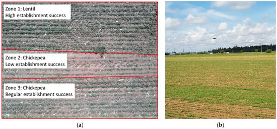
Figure 1.
Example of the three zones in the image gathered at 4 m of relative height (a) and a picture of the data gathering process (b).
3.2. Used Drone
Concerning the drone, as we want to develop a low-cost and scalable solution for the farmers, we focus on low-cost drones. We have to select a drone that allows gathering RGB images in a nadir mode. The drone we have selected is the Parrot Bebop 2 Pro [27], which can be seen during data gathering and after landing in Figure 2. This drone has an average flying autonomy of 20 min in normal conditions. Its weight is 504 g, which is relatively low considering that it has two cameras (the nadir and the frontal one). The nadir camera allows gathering RGB and thermal images. Although the gathered images have 1080 × 1440 pixels and 24-bit colour, we have reduced them to 8-bit colour to minimise their size in order to allow better storage.
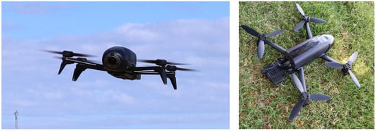
Figure 2.
Images of the drone in different moments of the data gathering process.
Images there captured at a different height. It is important to note that a higher height allows covering the same surface with fewer images. Moreover, it has a positive impact on flying time and energy consumption. The selected relative heights for the captured picture are 4, 8, and 12 m (606, 610, and 614 m of altitude). We have selected these heights based on [28].
3.3. Experimental Design and Statistical Analysis
The three zones defined in the previous subsection are divided into five subzones, having a total of 15 subzones. In Figure 3, we can see the included zones (and subzones) for the three flying heights. It is important to note that certain parts of the pictures might not be included to ensure similar establishment success conditions along the zones. More specifically, in the picture captured at 12 m, not all the image is used, as the establishment success is not homogenous for the upper part of the picture for Zone 1. This lack of homogeneity might be explained by differences in soil characteristics and problems in sowing or seeds. It is important to remark that classification into different zones are done based on the characteristics of the establishment success due to differences in species, sowing process, and field characteristics. We identified the zones with similar performance to create the three zones. The different zones can be seen in different colour (Zone 1 = black, Zone 2 = red, and Zone 3 = blue). Vertical lines of the same colours delimit the subzones. We generate the zones following this process to have a scenario as similar as possible to real conditions, in which it will be necessary to evaluate the establishment’s success and identify the areas with low performance.
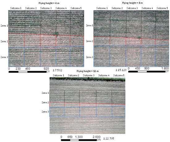
Figure 3.
The division into zones and subzones of the used images with scale and text bar.
Data for the different zones were subjected to factorial analyses of variance (ANOVAs) to test the effects of the three factors (flying height, cell size, and zone) in the percentage (%) of green plants. The procedure to have the % of the green plant is defined in the following subsection. Once we have confirmed that the zone affects the % of green plants of each sub-zone, we will use a single-factor ANOVA. This single-factor ANOVA is used to determine which aggregation cell (defined in the following section) ensures the use of data. We assume that data can be used as far as the ANOVA procedure differentiates data into three groups. If the result of the ANOVA is a p-value higher than 0.005 or the data is divided into two groups, we assume that generated information is not useful. The creation of groups is achieved using the Fishers Least Significant Difference (LSD). All the statistical analyses are performed with Statgraphics Centurion XVII [29].
3.4. Image Processing
To select image processing techniques, we based on the scheme used in the past to determine the presence of weed plants: application of an index and aggregation technique for the obtained results of the index [30]. The ArcMAP software was selected [31], but when the method is applied in the node, Python programming engine will run the operations with matrixes. A summary of the scheme can be seen in Figure 4. In this case, a simple index that combining the information of green and red bands differentiates between (i) green vegetation and (ii) soil and non-green vegetation is used. The remaining straw residuals, pebbles, soil or shadows are classified as the second type of coverage. The index can be seen in Equation (1). Based on the properties of the generated raster, only integer values are allowed. All the pixels of the resultant raster with value = 0 are considered green vegetation.
Index = B1/B2
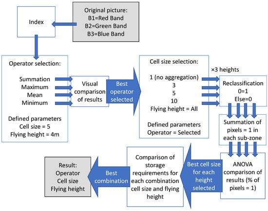
Figure 4.
Summary of the methodology followed in this paper.
Once the results of the index is obtained, we apply the aggregation technique. As an aggregating technique, we will compare the following operators: summation, maximum, mean, and minimum. Moreover, we include different cell sizes: 1 (no aggregation), 3, 5, and 10 pixels. We will compare the results of the different operators to select the best one using a single cell size and a single height.
Once the best operator is defined, we apply this operator with different cell sizes and heights. The rasters are then reclassified. For the reclassification, the pixel with a value of “0” (green plants) are classified as “1”, while the pixels with other values are classified as “0”. Following, each subzone’s summation of pixels with value = “1” is carried out to obtain the value that summarises each subzone. This value is used in the statistical analysis. We use an ANOVA procedure to compare the results and define which cell size and height combination is suitable. We select the combination that, maximising the cell size, allows the correct differentiation of the three groups in the ANOVA.
Finally, we compare the required storage capacity in Kbytes to store the resultant images of a given surface. We select a given surface of 1 Ha, representing 1154, 284, and 128 pictures for 4, 8, and 12 m of relative flying height.
4. Results
This section describes the obtained results in detail, both for the image processing and the classification with statistical analyses and ANN.
4.1. Selection of Best Operator and Cell Size
First and foremost, the comparison of usability of the aggregation operator is analysed. Figure 5 depicts different aggregation methods for the image gathered at 4 m with a cell size = 5. We can see the image in true colour (RGB image) the results of applying the index and the four rasters after the aggregation technique with different operators. The pixels with value = 0, black pixels, indicate the presence of vegetation.
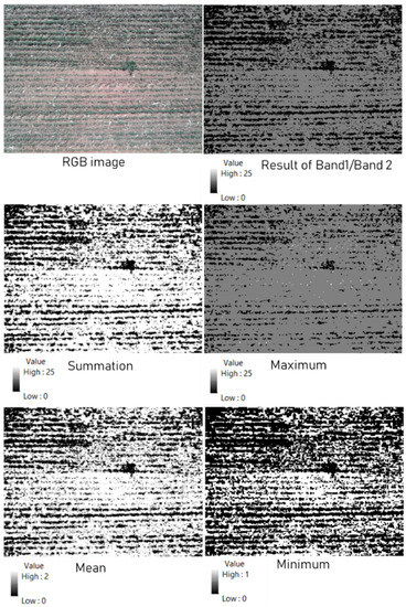
Figure 5.
Resultant raster after aggregation technique with different operators with cell size = 5 and relative flying height = 4 m.
At first sight, we can see that mean and minimum are not optimal, as they generate several false positives. We have considered as false positives the pixels with value = 0 (the value assigned for green vegetation) composed mainly by pixels of soil or other types of surface that are not green vegetation. To make this comparison, different portions of the picture in each zone are observed, comparing the index’s output and the output after aggregation. The operator equal to minimum was the one with the highest % of false positives followed by the operator equal to mean, summation and maximum. As we want to create a tool based on the most restrictive index, to avoid as much as possible the false positives, the operator maximum is selected.
Once the best operator is defined, we need to evaluate the cell size. We can see that as the pixel size increase, the range of possible values for the pixel (0 to 25 initially) decrease, reaching a range from 0 to 13 for cell size = 10. The portion of pixels with high values increase with the cell size too. In order to facilitate the observation of these results, Figure 6 is included. In Figure 6, we can see the results after the raster reclassification for every flying height and cell size. In brown, we can see the pixels with a value = 0. Meanwhile, the pixels with value = 1 (vegetation) are represented in green. In white rectangles are indicated the area covered in the image gathered at 4 m.
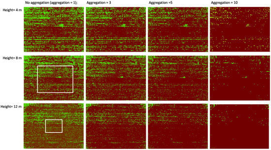
Figure 6.
Resultant raster after reclassification for all relative flying height and cell sizes.
In order to define the best cell size for each flying height, we calculate the % of pixels with value = 1 in each of the 15 subzones defined in the previous section. As we identify in Figure 6, the higher the height, the lower the % of pixels with value = 1. The same trend is observed when the aggregation cell size increases, finding in some cases sub-zones without any pixels with value = 1. This effect at 4 m is only seen with aggregation cell size = 10 for the Sub-zone 2. Meanwhile, for 8 and 12 m, we can identify this effect for an aggregation cell size of 5 for Sub-zone 2. This effect appears for all the sub-zones with an aggregation cell size of 10 and images gathered at 12 m.
After checking the results, we identify that some sub-zones identified initially as sub-zone 2 cannot be used, as the establishment success is similar to Sub-zone 3. Therefore, the values of these three sub-zones (1 sub-zone for a relative flying height of 8 m and two sub-zones of relative flying height of 12 m) are not included in the statistical analysis.
Following, in Figure 7, we outline the results of ANOVA and represent the variation of mean values for each combination of flying height and cell size. We can identify in a visual graphic the trends aforementioned (decrease of % of pixels = 1 as increase the flying height and the cell size). On the other hand, we present the p-value of the ANOVAs and the group creation. Our objective is that tool can distinguish between the three zones. The other values must be interpreted as not accurate enough. Our results indicate that for images collected at 4 m, the cell size of 1, 3, and 5 offered good performance. Meanwhile, images gathered at 8 m only offers acceptable performance for aggregation sizes of 1 and 3. Images at 12 m only can be used without aggregation, which means cell size = 1.
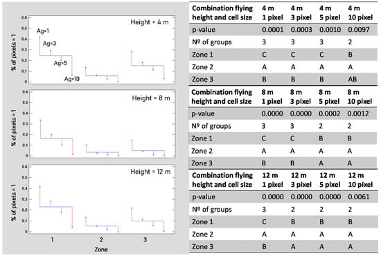
Figure 7.
Summary of ANOVA and visual representation of means.
To conclude this subsection, we have identified six combinations of flying height and aggregation cell size that offer results accurate enough to accomplish our requirements based on ANOVA results. We select maximum as the most appropriate operator for the aggregation technique. We will analyse which flying height and cell size combination minimise the storage requirements in the following subsection.
4.2. Comparison of Pairs of Flying Heigh and Cell Size
To analyse the balance between accuracy and resolution, we consider the size of the picture after the aggregation with different cell sizes. The sizes are 1.48 MB, 168.75 KB, 60.75 KB, and 15.19 KB for the aggregations’ cell sizes of 1, 3, 5, and 10. Next, we have to consider the number of pictures required to cover the given area. We assume 1154, 284, and 128 pictures to cover the surface of 1 Ha for 4, 8, and 12 m of relative flying height. With this data, we can calculate the storage requirements to store the resultant raster.
Figure 8 depicts the storage capacity needed to save the generated raster for a given area. The red “x” indicates the combinations that address the accuracy requirements, allowing subzones’ classification into three defined zones. Considering the required storage capacity for each of the aforementioned combinations, the one that minimises this capacity is 8 m and the cell size of 3 pixels. While the required storage for the images gathered at 8 m + cell size of 3 is 47.6 MB, for the other combinations are 68.45 KB (4 m + cell size = 5) and 104.1 KB (12 m + cell size = 1).
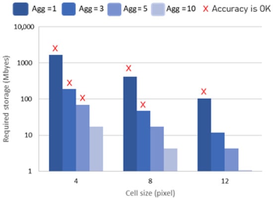
Figure 8.
Required storage capacity for each pair of flying height and cell size for 1 Ha. The x in red indicates what images can be used to differentiate the three zones.
Although this capacity seems small and might question the need for losing resolution to save storage capacity, the use of aggregation with a cell size of 5 has supposed a reduction of more than 95% of the required space compared with the original picture. For the field of 1 Ha monitored 4 m without aggregation techniques, the required storage capacity reaches 1667.8 MB compared with the 47.6 MB that we identify as the best combination.
4.3. ANN as an Alternative Classification Method
We include the generated data as input of ANN. With this analysis, we can evaluate the classification performance of data with different characteristics (aggregation and flying height). Moreover, this analysis is essential to endow our tool with a more powerful classification method. It must be noted that even that this is an artificial intelligence technique when the node will perform the method, the threshold established in this paper will be included, and no ANN should be processed.
Thus, the first step is to create the ANN formed by three input neurons (aggregation cell size, flying height, and % of pixels with value = 1) and three output neurons (high establishment success, mean establishment success, and low establishment success). These establishment success levels correspond to Zone 1, 3, and 2, respectively. We need to remark that the cases excluded in the statistical analysis are not included in the ANN. Thus, a total of 168 cases are included.
We have selected 120 aleatory cases to train the ANN and 48 cases to verify its accuracy. Table 1 shows the % of cases correctly classified in the training dataset. We can identify that the most common erroneous classifications are between Zone 1 and 3. In general terms, we have a correct classification of 80.83%. Zone 1 is the group with the highest number of cases used for the training (47), and Zone 2 is the one with the lowest number (33). This sharp difference is caused by the reduced number of observations for Zone 2. Regarding the % of correct classification of each zone, Zone 2 is the one with the highest % of correct classifications, and Zone 3 has the lowest %.

Table 1.
Percentage (%) of cases correctly classified in the training dataset.
According to the parameters defined in the training dataset, we classify the verification dataset. In this case, see Table 2, 83.33% of the cases are correctly classified with a percentage of 100% for Zone 1 and Zone 2. Zone 3 was wrongly classified as Zone 1 in 10% of cases and as Zone 3 in 30% of cases.

Table 2.
Percentage (%) of cases correctly classified in the verification dataset.
5. Discussion
In this section, we are going to discuss our results. First, we discuss using our data in conjunction with ANN to help farmers evaluate their legumes’ establishment success. Then we analyse the limitations of this study and its usefulness in the framework of the project GO TecnoGAR.
5.1. Further Use of the Results of ANN
The use of ANN in agriculture is not a new issue, and we can find several examples. Specifically, in image processing, it has been used for many purposes, such as identifying plant diseases [32] or yield estimations based on canopy cover and other parameters [33]. Nonetheless, the combined use of ANN with RGB images to compare the establishment success is no found. Examples in which graphical information generated from ANN is given to farmers to manage their lands can be found in [34,35].
To demonstrate the usefulness of the ANN and the generated data, we include an example. In Figure 9, we show the output for the ANN, or the classification, in a graphical form that can be used to classify other cases. Specifically, we represent the output for a relative flying height of 8 m, in which a given combination of % of pixels and cell size used can be combined to estimate the establishment success (high, medium, or low). This figure illustrates the possibility of classifying other pictures gathered at 8 m for different cell sizes according to their % of pixels = 1 (following the proposed methodology). It can be helpful when no ANN can be conducted by the device that gathers and processes the data, as in this proposal. This graphical classification includes the thresholds to be considered. In this case, for 8 m, ANN suggests using 0.6 and 0.17%. The images with less than 0.6% of pixels = 1 zones represent low establishment success, images between 0.6 and 0.17% zones with medium establishment success, and images above 17% zones with high establishment success. Another advantage of this graphic is that data has been extrapolated to predict the thresholds for other combinations.
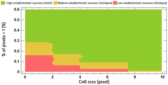
Figure 9.
Classification of ANN according to the % of pixels = 1 including variable cell size and fixed relative flying height of 8 m.
Concerning the success of the classification in the verification dataset, it is similar to the success obtained by other authors in the related work. In [18], the authors classify correctly 89% of cases based on histograms to estimate the plant growth. In a recent survey about machine learning in agriculture, most of the identified accuracies are between 80 and 100% [36]. Thus, our method has acceptable accuracy. This information is further exploited in Section 5.3.
5.2. Limitations of the Performed Study
The present paper has based on the pictures acquired during the initial period of leguminous crops growth. In this initial stage, it is difficult to differentiate between different species of legumes by their colour. Nonetheless, the establishment success itself is different, being the lentils, compared to chickpea, the one with the highest, fastest and more uniform establishment success. The present index cannot be used to differentiate between legumes species or varieties, but it can be used to compare the establishment success of different areas regardless of the species.
The major limitation of this study is that to keep the experimentation stage as operative as possible, we have reduced the flying high to three different values (4, 8, and 12 m). Moreover, the selected drone has a limited resolution, which is fixed given our low-cost objective. These analyses must be repeated with drones with better cameras and higher costs to obtain results for scenarios where no limitations are encountered. Thus, it can be evaluated if a camera with higher resolution and more flying height and cell size can find a new combination that reduces the storage requirements.
The second limitation of this study is that images are gathered in a single location, which means a reduced variability in the soil. Based on interviews with farmers performed under the GO TecnoGAR framework, we can identify a considerable variability in soil types. This variability might interfere with the correct classification of pixels. Nonetheless, we do not expect further problems related to the soil, as even with the huge variability (with and without straw, with and without pebbles, different organic matter contents, etc.) not one of the observed fields had green components that can be classified as vegetation. The weed plants might be a problem in some cases. This study includes weed plants, specifically in Zone 1, Sub-zone 3 and 2, and Zone 2 Sub-zone 4 (at 4 m, in other cases, check Figure 3), and no problems are detected. Nevertheless, in cases with a very high presence of weed plants, false-positive might affect the results of this tool. Thus, it is essential to find an index capable of differentiating the weed plants and crops.
Based on the presented data, the proposed tool is the preliminary version that will be enhanced by adding more scenario diversity and a higher range of establishment success performances. Other tools that use more powerful methods might be more accurate, as mentioned in the previous subsection. Nonetheless, for the purpose of this initial test, the archived accuracy (83% or accuracy) is high enough. The last limitation, which is justified based on our approach, is the conventional image processing instead of using machine vision techniques for the classification. We aimed to develop a simple tool that can operate in scenarios with no internet access and relatively low computation requirements (low-cost nodes).
5.3. Usefulness of Proposed Tool for the GO TecnoGAR
The main use of this methodology is the comparison of the establishment success performance of different varieties of chickpea or even between legumes based on their canopy cover in an early stage. In the case of GO TecnoGAR, during the coming years 2022 and 2023, we will have experimental plots with different chickpea varieties with several management settings (biostimulants, sowing patterns, etc.). This method aims to have a fast and trustable tool designed for legumes to compare the establishment success to evaluate the performance of different tested varieties. The proposed methodology will be implemented in a node with a camera similar to the one used in this paper and mounted in a drone. It will help to evaluate and compare the establishment success of the varieties without requiring high computational capacity or storage capacity. The tool can be operated in a Raspberry-type node without needing internet access for cloud computing, as the data will be computed in the edge. It will only require operating with matrixes and applying a threshold based on the results of the ANN analysis presented in this paper. These processes will be running in the node.
Table 3 depicts a comparison between the related work and the proposed approach. In this table, we summarise the main characteristics of our proposed solution and the existing ones. Thus, we can see that existing methodologies are adapted to other crops. The methods proposed in [20,21] followed a similar approach, Qualitative Classification (QlC). However, they were applied to a higher height, and considering the low coverage and slow growth of chickpea, they cannot be used. Another group of existing solutions [22,23,24,26] offered Quantitative Classifications (QnC), but requires higher computational capacity. Finally, Ref. [25] is based on a similar methodology, vegetation index and a threshold and offer quantitative results. However, it is based on data from a multi-spectral camera, and the price of the used sensor is up to EUR 6.700. The drone used to gather the pictures of this paper costs less than EUR 600. The provided accuracies can be based on the results of the classification or on linear regressions. In the second case, R2, is included to indicate that accuracy is based on the correlation coefficient.

Table 3.
Comparative performance and methodology of existing solutions.
The proposed methodology can be applied to pictures captured through a diverse range of devices. In most cases, images will be obtained with drones. Nonetheless, among the plots included in GO TecnoGAR we find several areas where drones cannot be operated due to legal restrictions. In these regions, farmland structures such as pivots will be used to install cameras.
There is no other specific tool for comparing or estimating establishment success in legumes or in other crops. Therefore, it was necessary to generate a specific methodology to estimate the establishment success before starting the experimental plans of the next years.
6. Conclusions
In this paper, we evaluate the possibility of using drone images with a simple image processing (index, aggregation technique, and threshold) to estimate the establishment success of legumes. The methodology is based on previous proposals in the field, designed to identify weed plants, and was adapted to detect vegetation in contrast with soil. Three zones with different establishment success are used to calibrate our tool. We include images gathered at 4, 8, and 12 m with different aggregation cell sizes in order to find the combination of the aforementioned parameters, which minimises the required storage capacity to save the data.
Our results indicate that the proposed methodology can differentiate regions of the picture with different establishment success performances correctly. Moreover, we identify the combination that, maintaining the accuracy, reduces the storage requirements. This combination is 8 m and aggregation cell size of 3 pixels. Finally, we show the usefulness of the proposed tool combined with ANN to establish a threshold that will be applied for the classification of the establishment success of the area.
Future work will include more flying height and aggregation cell size combinations with better cameras to evaluate if other combinations improve the required storage capacity established in this paper. Moreover, applying the proposed method to compare the establishment success of different chickpea varieties as a fast method to evaluate the performance of these varieties along with the cropping periods under the framework of GO TecnoGAR will be carried out. Thus, it will generate more images that will be used to improve the operation of the method by having a qualitative approach with more classes or even assess if it is possible to have a quantitative approach. After enhancing the method, comparison of its performance with other proposals based on artificial intelligence will be presented. Finally, the inclusion of more locations will nurture our database with a higher soil variability, enhancing the robustness of the proposed method.
Author Contributions
Conceptualisation, J.L.; methodology, L.P.; field measures and sampling, D.M.-C.; data curation, L.P.; writing—original draft preparation, L.P. and S.Y.; writing—review and editing, J.L.; supervision, J.F.M.; validation, P.V.M.; project administration, P.V.M. All authors have read and agreed to the published version of the manuscript.
Funding
This research and the contract of S.Y. were funded by project PDR18-XEROCESPED, under the PDR-CM 2014–2020, by the EU (European Agricultural Fund for Rural Development, EAFRD), Spanish Ministry of Agriculture, Fisheries and Food (MAPA) and Comunidad de Madrid regional government through IMIDRA and the contract of L.P. was funded by Conselleria de Educación, Cultura y Deporte with the Subvenciones para la contratación de personal investigador en fase postdoctoral, APOSTD/2019/04.
Institutional Review Board Statement
Not applicable.
Informed Consent Statement
Not applicable.
Data Availability Statement
The data presented in this study are available on request from the corresponding author. The data are not publicly available due to privacy constrains.
Conflicts of Interest
The authors declare no conflict of interest.
References
- FAO. The Future of Food and Agriculture—Alternative Pathways to Rome; FAO: Rome, Italy, 2018; p. 224. [Google Scholar]
- Maes, W.H.; Steppe, K. Perspectives for remote sensing with unmanned aerial vehicles in precision agriculture. Trends Plant Sci. 2019, 24, 152–164. [Google Scholar] [CrossRef]
- Tsouros, D.C.; Bibi, S.; Sarigiannidis, P.G. A review on UAV-based applications for precision agriculture. Information 2019, 10, 349. [Google Scholar] [CrossRef]
- Vasilean, I.; Cîrciumaru, A.; Garnai, M.; Patrascu, L. The influence of light wavelength on the germination performance of legumes. Ann. Univ. Dunarea Jos Galati Fascicle VI Food Technol. 2018, 42, 95–108. [Google Scholar]
- Yadav, V.L.; Shukla, U.N.; Raiger, P.R.; Mandiwal, M. Efficacy of pre and post-emergence herbi-cides on weed control in chickpea (Cicer arietinum L.). Indian J. Agric. Res. 2019, 53, 112–115. [Google Scholar]
- Khan, I.A.; Khan, R.; Jan, A.; Shah, S.M.A. Studies on tolerance of chickpea to some pre and post-emergence herbicides. Emir. J. Food Agric. 2018, 30, 725–731. [Google Scholar] [CrossRef]
- Wahab, I.; Hall, O.; Jirström, M. Remote sensing of yields: Application of uav imagery-derived ndvi for estimating maise vigor and yields in complex farming systems in sub-saharan africa. Drones 2018, 2, 28. [Google Scholar] [CrossRef]
- Lan, Y.; Deng, X.; Zeng, G. Advances in diagnosis of crop diseases, pests and weeds by UAV re-mote sensing. Smart Agric. 2019, 1, 1. [Google Scholar]
- Ballesteros, R.; Intrigliolo, D.S.; Ortega, J.F.; Ramírez-Cuesta, J.M.; Buesa, I.; Moreno, M.A. Vineyard yield estimation by combining remote sensing, computer vision and artificial neural network techniques. Precis. Agric. 2020, 21, 1242–1262. [Google Scholar] [CrossRef]
- Quebrajo, L.; Perez-Ruiz, M.; Pérez-Urrestarazu, L.; Martínez, G.; Egea, G. Linking thermal imaging and soil remote sensing to enhance irrigation management of sugar beet. Biosyst. Eng. 2018, 165, 77–87. [Google Scholar] [CrossRef]
- Akbal, A.; Akbal, E. Scalable Data Storage Analysis and Solution for Picture Archiving and Communication Systems (PACS). Int. J. Inf. Electron. Eng. 2016, 6, 285–288. [Google Scholar] [CrossRef][Green Version]
- Delgado, J.A.; Short, N.M., Jr.; Roberts, D.P.; Vandenberg, B. Big data analysis for sustainable agriculture on a geospatial cloud framework. Front. Sustain. Food Syst. 2019, 3, 54. [Google Scholar] [CrossRef]
- Parra, L.; Marin, J.; Yousfi, S.; Rincón, G.; Mauri, P.V.; Lloret, J. Edge detection for weed recognition in lawns. Comput. Electron. Agric. 2020, 176, 105684. [Google Scholar] [CrossRef]
- El-Sayed, H.; Sankar, S.; Prasad, M.; Puthal, D.; Gupta, A.; Mohanty, M.; Lin, C.-T. Edge of Things: The Big Picture on the Integration of Edge, IoT and the Cloud in a Distributed Computing Environment. IEEE Access 2017, 6, 1706–1717. [Google Scholar] [CrossRef]
- Silva, G.R.; Escarpinati, M.C.; Abdala, D.D.; Souza, I.R. Definition of Management Zones through Image Processing for Precision Agriculture. In 2017 Workshop of Computer Vision (WVC); IEEE: Piscataway, NJ, USA, 2017; pp. 150–154. [Google Scholar]
- Ahmad, N.; Iqbal, J.; Shaheen, A.; Ghfar, A.; Al-Anazy, M.M.; Ouladsmane, M. Spatio-temporal analysis of chickpea crop in arid environment by comparing high-resolution UAV image and LANDSAT imagery. Int. J. Environ. Sci. Technol. 2021, 1–16. [Google Scholar] [CrossRef]
- Marsujitullah; Manggau, F.X.; Parenden, D. Interpretation of Food Crop Growth Progress Visualization and Prediction of Drone Based Production Estimates Based on Histogram Values in Government Areas-Case Study of Merauke Regency. In Proceedings of the IOP Conference Series: Materials Science and Engineering, Makassar, Indonesia, 16–17 October 2020. [Google Scholar]
- Marsujitullah, M.; Xaverius Manggau, F.; Rachmat, R. Classification of Paddy Growth Age Detection Through Aerial Photograph Drone Devices Using Support Vector Machine And Histogram Methods, Case Study Of Merauke Regency. Int. J. Mech. Eng. Technol. 2019, 10, 1850–1859. [Google Scholar]
- Panday, U.S.; Shrestha, N.; Maharjan, S.; Pratihast, A.K.; Shahnawaz; Shrestha, K.L.; Aryal, J. Correlating the Plant Height of Wheat with Above-Ground Biomass and Crop Yield Using Drone Imagery and Crop Surface Model, A Case Study from Nepal. Drones 2020, 4, 28. [Google Scholar] [CrossRef]
- Murugan, D.; Garg, A.; Singh, D. Development of an Adaptive Approach for Precision Agriculture Monitoring with Drone and Satellite Data. IEEE J. Sel. Top. Appl. Earth Obs. Remote. Sens. 2017, 10, 5322–5328. [Google Scholar] [CrossRef]
- Agarwal, A.; Singh, A.K.; Kumar, S.; Singh, D. Critical analysis of classification techniques for precision agriculture monitoring using satellite and drone. In Proceedings of the 13th International Conference on Industrial and Information Systems (ICIIS), Rupnagar, India, 1–2 December 2018; pp. 83–88. [Google Scholar]
- Jin, X.; Liu, S.; Baret, F.; Hemerlé, M.; Comar, A. Estimates of plant density of wheat crops at emergence from very low altitude UAV imagery. Remote. Sens. Environ. 2017, 198, 105–114. [Google Scholar] [CrossRef]
- Ranđelović, P.; Đorđević, V.; Milić, S.; Balešević-Tubić, S.; Petrović, K.; Miladinović, J.; Đukić, V. Prediction of soybean plant density using a machine learning model and vegetation indices extracted from RGB images taken with a UAV. Agronomy 2020, 10, 1108. [Google Scholar] [CrossRef]
- Habibi, L.; Watanabe, T.; Matsui, T.; Tanaka, T. Machine Learning Techniques to Predict Soybean Plant Density Using UAV and Satellite-Based Remote Sensing. Remote Sens. 2021, 13, 2548. [Google Scholar] [CrossRef]
- Stroppiana, D.; Pepe, M.; Boschetti, M.; Crema, A.; Candiani, G.; Giordan, D.; Monopoli, L. Estimating crop density from multi-spectral uav imagery in maise crop. Int. Arch. Photogramm. Remote Sens. Spat. Inf. Sci. 2019. [Google Scholar] [CrossRef]
- Zhao, B.; Zhang, J.; Yang, C.; Zhou, G.; Ding, Y.; Shi, Y.; Liao, Q. Rapeseed seedling stand counting and seeding performance evaluation at two early growth stages based on unmanned aerial vehicle imagery. Front. Plant Sci. 2018, 9, 1362. [Google Scholar] [CrossRef]
- Specifications of Prarrot BeBop 2 Pro. Available online: https://s.eet.eu/icmedia/mmo_35935326_1491991400_5839_16054.pdf (accessed on 16 April 2021).
- Marin, J.F.; Mostaza-Colado, D.; Parra, L.; Yousfi, S.; Mauri, P.V.; Lloret, J. Comparison of performance in weed detection with aerial RGB and thermal images gathered at different height. In Proceedings of the ICNS 2021: The Seventeenth International Conference on Networking and Services, Porto, Portugal, 18–22 April 2021; pp. 1–6. [Google Scholar]
- Statgraphics Centurion XVIII. Available online: https://www.statgraphics.com/download (accessed on 6 July 2021).
- Parra, L.; Parra, M.; Torices, V.; Marín, J.; Mauri, P.V.; Lloret, J. Comparison of single image processing techniques and their combination for detection of weed in Lawns. Int. J. Adv. Intell. Syst. 2019, 12, 177–190. [Google Scholar]
- ArcMap|ArcGIS Desktop. Available online: https://desktop.arcgis.com (accessed on 6 July 2021).
- Sivasakthi, S.; MCA, M. Plant leaf disease identification using image processing and svm, ann classifier methods. In Proceedings of the International Conference on Artificial Intelligence and Machine learning, Vancouver, BC, Canada, 30–31 May 2020. [Google Scholar]
- García-Martínez, H.; Flores-Magdaleno, H.; Ascencio-Hernández, R.; Khalil-Gardezi, A.; Tijerina-Chávez, L.; Mancilla-Villa, O.; Vázquez-Peña, M. Corn Grain Yield Estimation from Vegetation Indices, Canopy Cover, Plant Density, and a Neural Network Using Multispectral and RGB Images Acquired with Unmanned Aerial Vehicles. Agriculture 2020, 10, 277. [Google Scholar] [CrossRef]
- Parra, L.; Botella-Campos, M.; Puerto, H.; Roig-Merino, B.; Lloret, J. Evaluating Irrigation Effi-ciency with Performance Indicators: A Case Study of Citrus in the East of Spain. Agronomy 2020, 10, 1359. [Google Scholar] [CrossRef]
- Li, Y.; Chao, X. ANN-Based Continual Classification in Agriculture. Agronomy 2020, 10, 178. [Google Scholar] [CrossRef]
- Sharma, A.; Jain, A.; Gupta, P.; Chowdary, V. Machine Learning Applications for Precision Agriculture: A Comprehensive Review. IEEE Access 2020, 9, 4843–4873. [Google Scholar] [CrossRef]
Publisher’s Note: MDPI stays neutral with regard to jurisdictional claims in published maps and institutional affiliations. |
© 2021 by the authors. Licensee MDPI, Basel, Switzerland. This article is an open access article distributed under the terms and conditions of the Creative Commons Attribution (CC BY) license (https://creativecommons.org/licenses/by/4.0/).