Estimation of Winter Wheat Yield from UAV-Based Multi-Temporal Imagery Using Crop Allometric Relationship and SAFY Model

Abstract

Crop yield prediction and estimation play essential roles in the precision crop management system. The Simple Algorithm for Yield Estimation (SAFY) has been applied to Unmanned Aerial Vehicle (UAV)-based data to provide high spatial yield prediction and estimation for winter wheat. However, this crop model relies on the relationship between crop leaf weight and biomass, which only considers the contribution of leaves on the final biomass and yield calculation. This study developed the modified SAFY-height model by incorporating an allometric relationship between ground-based measured crop height and biomass. A piecewise linear regression model is used to establish the relationship between crop height and biomass. The parameters of the modified SAFY-height model are calibrated using ground measurements. Then, the calibrated modified SAFY-height model is applied on the UAV-based photogrammetric point cloud derived crop height and effective leaf area index (LAIe) maps to predict winter wheat yield. The growing accumulated temperature turning points of an allometric relationship between crop height and biomass is 712 °C. The modified SAFY-height model, relative to traditional SAFY, provided more accurate yield estimation for areas with LAI higher than 1.01 m²/m². The RMSE and RRMSE are improved by 3.3% and 0.5%, respectively.

1. Introduction

Crop biomass is an important parameter for crop yield potential prediction. Environmental conditions such as solar energy, temperature, soil nutrients, water, pests, disease, weeds, and other stresses can affect dry aboveground biomass (DAM) and potential yield of a crop [1]. As a crop management system, precision farming emphasizes monitoring and analysis to help farmers achieve optimal profit [2]. Hence, precision farming focused on targeted and cost-effective inputs to enhance efficiency and sustainability outputs. Therefore, mapping field-scale crop DAM play an essential role in precision farming. Conventional crop yield estimation methods are labor intensive and have limited sampling numbers due to the accessibility of fieldwork. These methods provide rough estimations and advising in farming activities. Remote sensing technology allows monitoring of variability for large-scale fields without a large amount of ground data. For example, satellite remote sensing has been used for regional crop monitoring. However, satellite imagery is hampered by long revisit times and cloud presence. Additionally, the cost of high temporal and spatial resolution satellite imagery limits its use. Unmanned Aerial Vehicle (UAV) collected high spatial and temporal imagery can monitor within-field DAM and yield variability in real-time. However, a practical and accurate approach is required to achieve within-field crop biomass monitoring and estimation using UAV-based data.

Two approaches have been adopted using remote sensing technology to estimate crop biomass. The first category is the statistical model, which uses the relationship between remote sensing vegetation indices and in-situ crop biomass measurements to estimate crop biomass [3,4,5]. The UAV-based high spatial resolution remote sensing data can indicate the crop biomass variation within the field using the vegetation indices. However, this method is applicable only for specific crop growth stages and geographic location, and variations in environmental conditions and location will affect the accuracy [6]. The second category is the crop growth model, which uses crop and environment parameters to simulate the development of crop growth and estimate crop biomass. Currently, crop growth models such as AquaCrop [7], CERES [6,8], STICS [9], CropSyst [10], and WOFOST [11] have been well developed in crop production estimation. However, these models require a comprehensive set of parameters to simulate crop growth status, which is difficult to collect and use for within-field DAM and yield estimation. WOFOST is a labor and time-intensive model which requires about 40 parameters, and may not be an affordable approach for UAV-based imagery in estimating within-field crop yield.

An allometric method is an alternative approach for estimating plant biomass from other crop parameters. Plants absorb solar energy and transfer this energy to biomass during the growing season. The allocation pattern of the biomass distribution between stem, leaves, fruit, and roots follows a special allocation principle for specific species. This pattern of energy allocation plays an essential role in the plant’s reproduction, which affects the final yield in cereal crops [12]. The plant’s allocation principle was defined as the allometric relationship in the plant, which is a part of the plant that has a similar variation rate compared with other parts of the plant or whole plant [13,14]. The information derived from the crop allometric relationships can also help farmers to monitor, analyze, and determine crop growth situations. Many remote sensing studies have proved that the allometric method can be applied to different crop species to determine the crop parameters [15,16,17,18]. The allometric method initially requires extensive destructive samplings to build an allometric model. The model could then be used as a non-destructive method to estimate crop biomass. Bakhshandeh et al., (2012) [14] addressed the allometric relationship between winter wheat plant height and biomass based on a ground-based study. However, limited ground sampling points presents a challenge for applying the allometric relationship to the entire field and displaying the within-field biomass variability.

Since intensive crop height data is either difficult or expensive to obtain from the conventional remote sensing methods such as satellite or airborne optical data directly, not many studies estimate crop biomass from plant height using remote sensing technology at a subfield scale. The recent development of the UAV system and computer vision have made possible dense 3D reconstructions to produce orthomosaic aerial image, DEM, and 3D photogrammetric point clouds using the Structure from Motion (SfM) method from UAV data. SfM is a computer vision technique that incorporates multi-view stereo images to match features, derive 3D structure, and estimate camera position and orientation. The SfM approach has been proven to be able to estimate of crop structural information such as, canopy size, height, and leave shape [19,20,21,22]. For example, Bendig (2014) [21] used a crop surface model to estimate the height of barley, highly correlated with the dry aboveground biomass. Thus, the allometric relationship between crop height and biomass could be meaningful information in estimating crop biomass.

A Simple Algorithm for Yield Estimation (SAFY) model uses the allometric relationship between daily crop leaf area index (LAI) and biomass accumulation to simulate the crop growth stages. In addition, it uses light use efficiency theory to determine the optimal parameters and estimate the final dry aboveground biomass of crops [18,23,24,25]. Song et al., (2020) [26] used the UAV-based Simulated Observation of Point Cloud (SOPC) derived effective leaf area index (LAIe) [27] and the SAFY model to generate the fine-resolution final DAM and yield maps of winter wheat. The SAFY model may be used to derive a more accurate final DAM and yield estimation by combining the allometric relationship between winter wheat canopy height and biomass. The objective of this study is to incorporate the allometric relationship between crop canopy height and biomass into the SAFY model and assess the accuracy of crop biomass estimation. A modified SAFY-height model will be developed and calibrated using ground-based measurements. The final DAM and yield will be estimated from the calibrated modified SAFY-height model using UAV-based canopy height and LAIe maps. The canopy height and LAIe maps of winter wheat will be generated using the moving cuboid filter [28] and SOPC method [27].

2. Materials and Methods

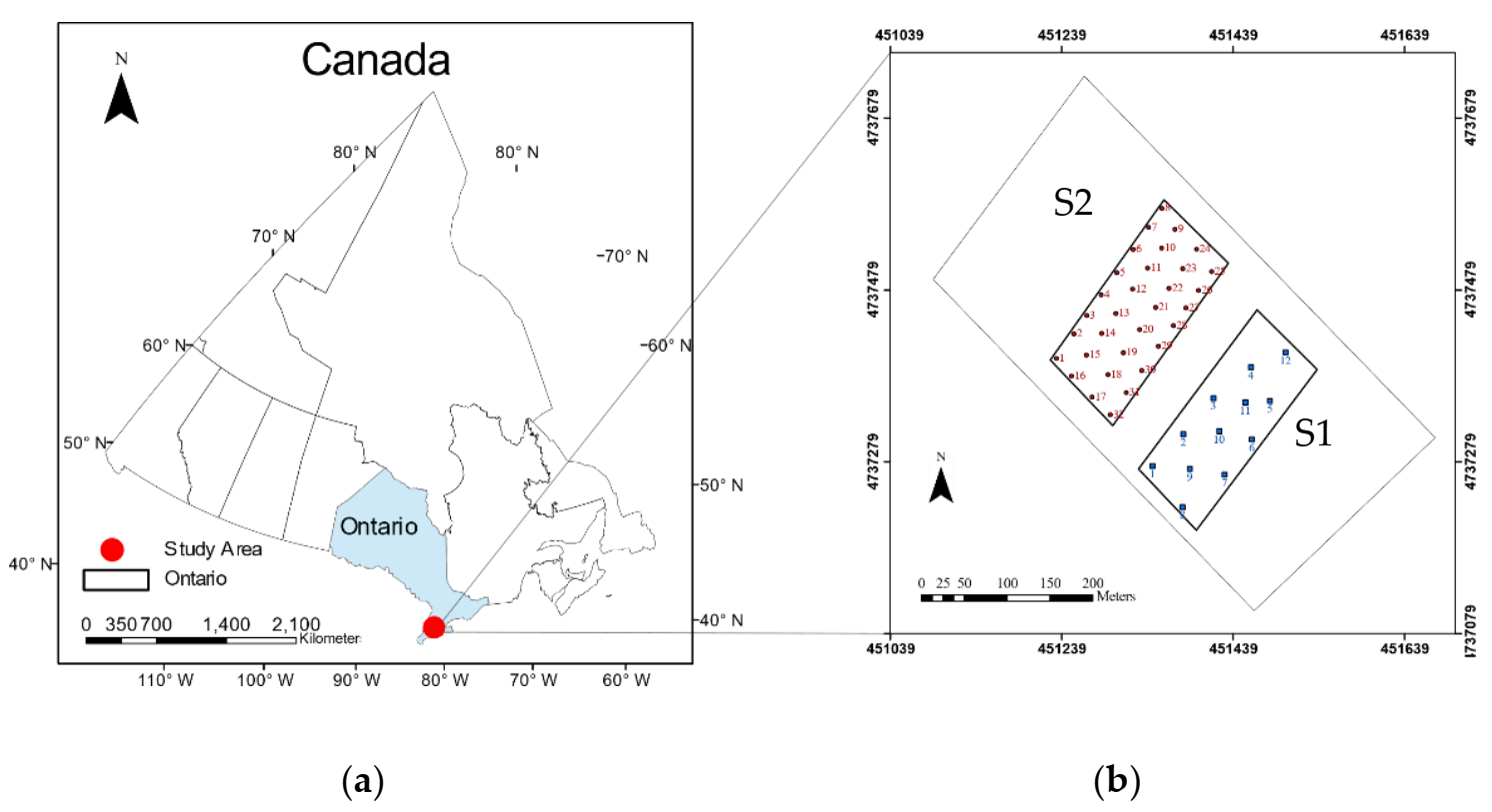
2.1. Study Area

The study site locates in the west of Melbourne, Southwest Ontario, Canada (42.787707°, –81.594801°). Since the study region has a shorter growing season, which can support one harvest per year, the soft red winter wheat (Brevatn Branson, Corteva Agriscience, USA) was seeded in October 2018 and harvested in July 2019. Two sub-fields were selected to collect different parameters. The size of the sub-field is 100 m by 200 m. The sub-fields are shown in Figure 1. The blue points are the sampling points in sub-field 1 (S1), and the red points are the sampling points in sub-field 2 (S2).

2.2. Ground Data Collection

The ground crop parameters collections were divided into two sub-fields since the destructive DAM will affect the accuracy of the UAV-based LAIe and height data. These two sub-fields were selected from one winter wheat field with the same cultivar, phenology, and nutrition supplies. S1 was used to collect winter wheat DAM, canopy height, LAIe, and final yield in 12 sampling locations. The Normalized Difference Water Index (NDWI) map derived from the Sentinel 2 imagery on 22 April 2019 was used for the selection of sampling locations. The NDWI map represents the water distribution of our study site, which will lead to a significant variation of crop final yield. S2 was used to collect winter wheat canopy height, LAIe, and final yield in 32 sampling locations. S2 used systematic sampling method to evaluate model performance. In addition, the UAV-based imagery was collected in S2. Multiple days of field work were conducted from 8 May to 20 July in 2019. The detailed parameters and dates are shown in

Table 1. The data collection in S1 and S2, including dry aboveground biomass (DAM), canopy height, effective leaf area index (LAIe), UAV imagery, and Biologische Bundesanstalt, Bundessortenamt und CHemische Industrie (BBCH).

	DAM (S1)	DAM (S2)	Canopy Height & LAIe (S1)	Canopy Height & LAIe (S2)	UAV Imagery (S2)	BBCH
8-May	12 samples		12 samples			20
11-May				32 samples	1257 images	21
17-May	12 samples		12 samples	32 samples		25
21-May	12 samples		12 samples	32 samples	1157 images	31
27-May	12 samples		12 samples	32 samples	1157 images	39
3-Jun	12 samples		12 samples	32 samples		49
11-Jun	12 samples		12 samples	32 samples		65
16-Jun						69
20-Jul	12 samples	32 samples	12 samples			85

. The DAM was collected from two blocks of a 0.5 m by 0.5 m section within a 2 m by 2 m area of each sampling location. After collecting the fresh winter wheat sample, the sample was transferred to the lab and oven dried at 80 °C for 24 h. The final dry weight of crop biomass was measured in the lab. The LAIe was calculated from the digital hemispherical photograph using the CAN-EYE v6.1. The digital hemispherical photograph was collected by a Nikon D300s camera and a 10.5 mm fisheye lens following the procedures described in Shang et al. (2014) [29]. The average crop canopy height was averaged from 10 measurements around the sampling location within a 2-m radius.

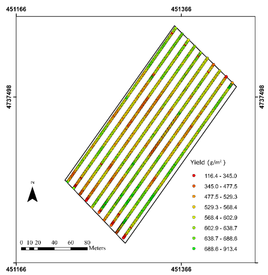
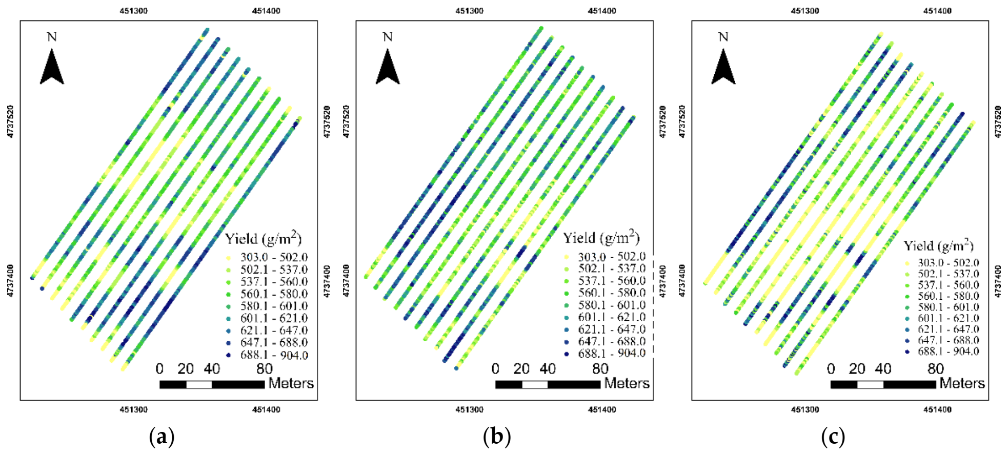
2.3. Combine Harvester Yield Data Collection

The crop final yield data comes from a John Deere combine harvester at the end of the season. The combine harvester had a 10 m wide head to collect the plant. The built-in real-time kinematic (RTK)-global navigation satellite system (GNSS) recorded the distance of the harvester moved every second. The area of the harvester moved will be calculated using the width of the head and driven distance. The grain yield monitor on the harvester recorded the grain weight, mass flow, and moisture content. The spatial yield map was composed of many points, which were shown in Figure 2. ArcMap 10.7 (ESRI, Redlands, CA, USA) was used to process the final yield data, including outlier removal, resampling, and data extraction.

2.4. UAV-Based Image Collection

A DJI Phantom 4 RTK UAV system was used to collect RGB imagery for S2 on 11 May, 21 May, and 27 May. The crop phenology for these dates at the BBCH scale was 21, 31, and 39, which covered the leaf development stage to the booting stage. The Phantom 4 RTK system can provide a 20MPix high-resolution imagery, and a ground RTK base station can achieve very high accuracy positional information. All UAV flights were performed at the altitude of 30 m with front and side overlapping of 90%. The UAV images have been processed to generate 3D point cloud data using Pix4Dmapper Pro v2.4 (Pix4D, Lausanne, Switzerland). The total processing time of photogrammetric point cloud generation is 30 h using a Windows computer with a 12 core Xeon cup and Quadro m4000 graphic card. The final resolution of the aerial image is 0.8 cm, and the point density of point cloud data is more than 4000 points/m².

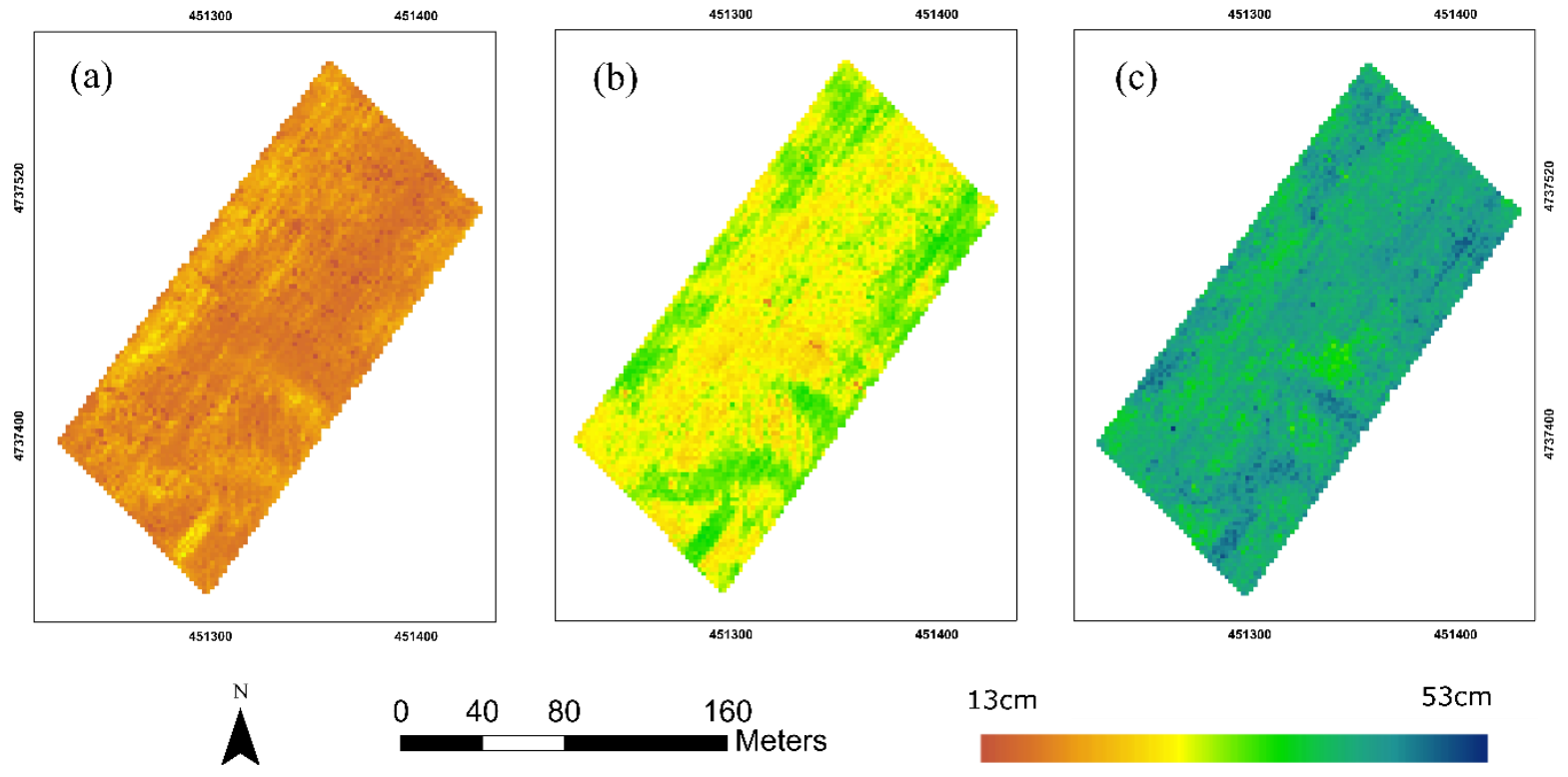
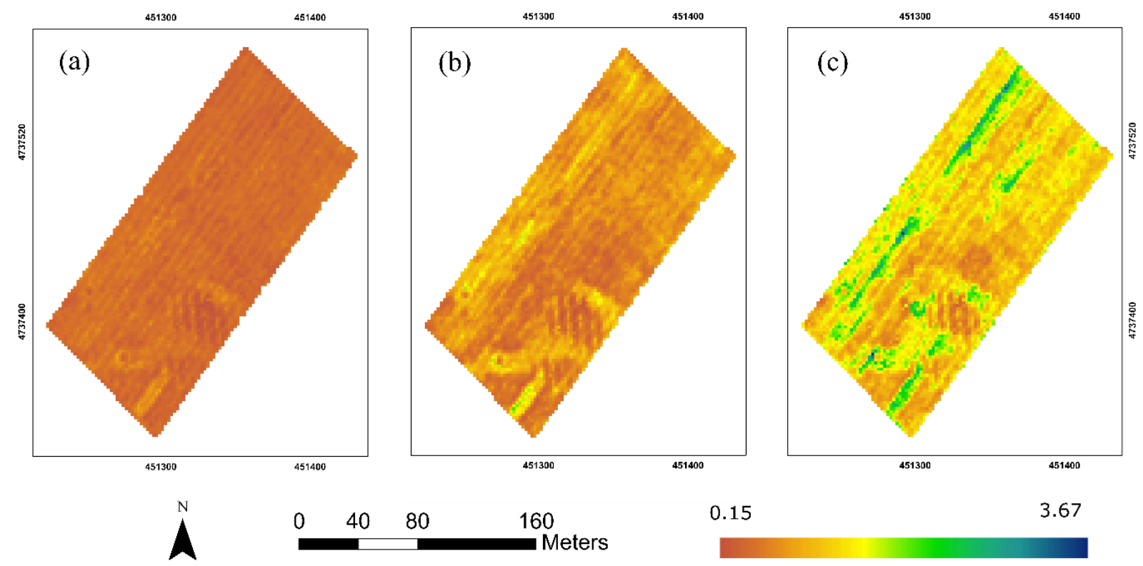
2.5. UAV-Based Plant Height and LAIe Maps

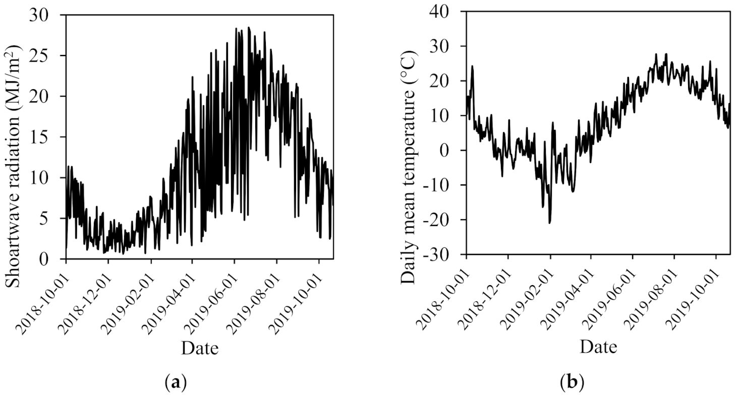
The UAV-based 3D point cloud data were used to generate the plant height and LAIe maps for three UAV operation days. The recently developed moving cuboid filter was used to retrieve the winter wheat plant height using the UAV-based 3D photogrammetric point cloud data without in-situ measurements [28]. The UAV-based photogrammetric point cloud data has very high point density with more than 4000 points/m². The final resolution of the products derived from photogrammetric point cloud data can be adjusted based on the research requirement [27,28]. The spatial resolution of canopy height and LAIe maps in this study was 2 m. In addition, the photogrammetric point cloud data can generate canopy height and LAIe maps of winter wheat with high accuracy in the early growth stages. The canopy height maps of winter wheat in S2 were shown in Figure 3. The root mean square error (RMSE) for each canopy height map was 2.61 cm, 3.65cm, and 4.17 cm for the three dates respectively. The overall RMSE for all ground measurements on three dates was 3.48 cm. The LAIe maps of winter wheat in S2 were shown in Figure 4. The overall RMSE for all ground measurements on three dates was 0.19.

The recent developed SOPC method was designed to estimate winter wheat LAIe from UAV-based 3D point cloud data using the gap fraction theory without in-situ measurements [26]. This method can successfully generate winter wheat LAIe maps at early growth stages from the leaf development to the booting stage. The UAV-based SOPC derived LAIe (SOPC-LAIe) maps are shown in Figure 4.

2.6. Weather Data

Weather data comes from a weather station located on the main campus of Western University, London, Ontario, which is 35 km away from the study site. The weather station collected the shortwave solar radiation and air temperature every 30 min. The daily shortwave solar radiation and the average air temperature were calculated; the data chart is shown in Figure 5.

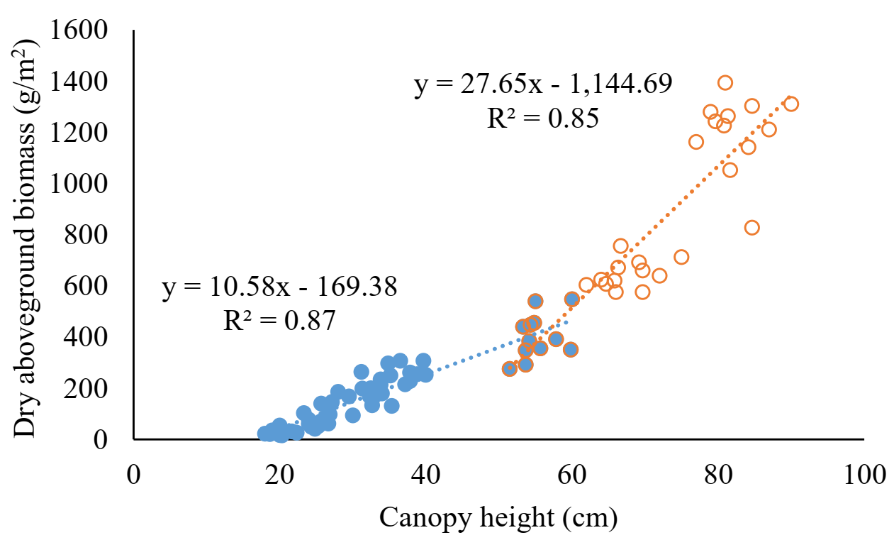
2.7. Allometric Relationship Establishment

A piecewise linear regression model has been used to determine the relationship between plant height and DAM on wheat [14]. The wheat growth can be separated into two phases. The first phase covers the tillering and stems elongation stages; the second phase covers the rest of the stages beyond the stem elongation stages. The equations are shown below:

$$DAM = a_1 \times H + b_1 if \sum T_a \le T_{turn},$$

$$DAM = a_2 \times H + b_2 if \sum T_a > T_{turn},$$

(1)

where DAM is the final dry aboveground biomass, H is the plant height, ${\alpha }_1$ is the increasing rate of DAM to H in the first phase, $b_1$ is the intercept in phase 1, $a_2$ is the increasing rate of DAM to H in the second phase, $b_2$ is the intercept in phase 2, the $\sum T_a$ is the sum of optimal air temperature accumulated since plant emergence, $T_{turn}$ is the turning point between the two phases which is the total accumulated temperature.

2.8. SAFY Model

The SAFY model has been used to simulate the winter wheat daily DAM and green leave area index (GLAI) during the growing season based on the crop LUE and leaf partitioning function theories [18,30,31]. The LUE theory is modelled below:

$$∆DAM = ELUE \times Rg \times {\epsilon }_C \times \left(1 - e^{-k \times GLAI}\right) \times F_T\left(T_a\right),$$

(2)

where $ELUE$ is the effective LUE; $Rg$ is the incoming shortwave solar radiation; ${\epsilon }_C$ is the climate coefficient, which ${\epsilon }_C$ = 0.48 [32,33,34]; the light-interception coefficient $k$ is 0.5 under the assumption of the leaf angle distribution is uniform and the leaf inclination is a spherical distribution [35,36]; and $F_T\left(T_a\right)$ is the temperature stress.

The daily increase of GLAI ($∆GLAI$) can be calculated from the fraction of the daily DAM ($∆DAM)$ which is portioned to leaves ($P_L$) according to a given coefficient of specific leaf area ($SLA$). The leaf partitioning function shows below:

$$∆GLAI = ∆DAM \times P_{L }(\sum T_a) \times SLA,$$

(3)

where $P_{L }$ is the fraction between leaf and dry aboveground biomass, which is determined by air temperature and another two parameters ($P_{La }$ and $P_{Lb }$) [31]. The equation can be written as follows:

$$P_{L }(\sum T_a) = 1 - P_{La }\times e^{P_{Lb}\sum T_a}$$

(4)

After the air temperature reached the threshold $S_{TT}$, the GLAI can be calculated from the following equation:

$$\mathrm{If}\sum T_a > S_{TT}$$

$$∆GLAI = GLAI \times \left(\sum T_a - S_{TT}\right)/Rs,$$

(5)

where $Rs$ is the rate of senescence.

After simulating the final DAM, the final crop yield can be calculated by multiplying the harvest index with the DAM. The final estimated yield was compared with the harvester measured yield to evaluate the performance of this study. The harvest index ($HI$) was calculated from the ground biomass and final yield in field 1, the average for all 12 sample points was 0.45. The equation shows below:

$$YIELD = DAM \times HI.$$

(6)

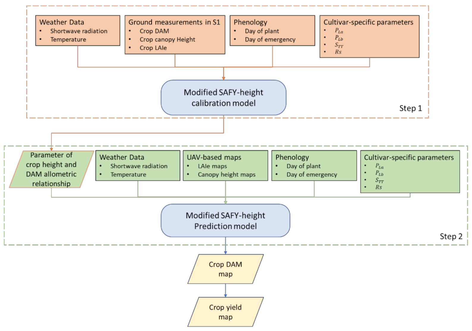
2.9. Modified SAFY-Height Model

The allometric relationship between crop canopy height and DAM is added to SAFY model to develop the modified SAFY-height model. This model is able to simulate a relationship between daily GLAI, canopy height, and DAM. First, the modified SAFY-height model will be calibrated using the ground-based DAM and canopy height measurements to determine the optimal parameters of the canopy height and DAM allometric relationship in S1 using the global optimization method, Shuffled Complex Evolution-University of Arizona (SCE-UA) algorithm [37]. In step one, Song et al. used the LAIe map derived from the UAV-based photogrammetric point cloud data to replace the GLAI and determined the cultivar-specific parameters ($P_{La}$, $P_{Lb}$, $S_{TT}$, $Rs$) [26]. In step two, the modified SAFY-height model will combine the UAV-based canopy height map, UAV-based LAIe map, the cultivar-specific parameters, and allometric relationship parameters derived from step one to simulate the final DAM. The general flow chart was shown Figure 6. Both LAIe and canopy height data will be used to calibrate the modified SAFY-height model and calculate cost function. The cost function combines both the RMSE of crop LAIe and canopy height. The equation is shown as (Equation (7)):

$$\mathrm{Cost}\mathrm{function}={\left[\frac{1}{N}{\displaystyle \sum }_{i=1}^N{\left(GLA{I}_{sim} - GLA{I}_{true}\right)}^2\right]}^{\frac{1}{2}} \times {\left[\frac{1}{N}{\displaystyle \sum }_{i=1}^N{\left(Heigh{t}_{sim} - Heigh{t}_{true}\right)}^2\right]}^{\frac{1}{2}}$$

(7)

According to the results of Song’s study [26], the cultivar-specific parameters were determined. The details are shown in

Table 2. SAFY parameters and associated values used in this study.

Parameter Name	Notation	Unit	Range	Value	Source
Climatic efficiency	${\epsilon }_C$	-		0.48	[30,31,32]
Temperature range for winter wheat growth	$T_{min}$, $T_{opt}$, $T_{max}$	°C		[0,25,30]	[23,32]
Specific leaf area	$SLA$	m2/g		0.022	[23]
Initial dry aboveground biomass	$DA{M}_0$	g/m2		4.2	[18,23]
Light-extinction coefficient	$k_{ext}$	-		0.5	[18,23]
Day of plant emergence	$DOE$	day		64	In-situ measurement
Day of senescence	$DOS$	day		284	In-situ measurement
Daily shortwave solar radiation	$Rg$	MJ/m2/d			In-situ measurement
Daily mean temperature	$T_{air}$	°C			In-situ measurement
Partition to leaf function parameter a	$P_{La}$	-		0.2608	[26]
Partition to leaf function: parameter b	$P_{Lb}$	-		0.0015	[26]
Sum of temperature for senescence	$S_{TT}$	°C		1080.96	[26]
Rate of senescence	$Rs$	°C day		2475.48	[26]
Effective light-use efficiency	$ELUE$	g/MJ	1.5–3.5		Variable in this study Range [18,23]

.

3. Results

3.1. Allometric Relationship between Plant Height and DAM

The DAM ranged from 15 to 1393 g/m², and the plant height ranged from 18 to 90 cm for S1 from 8 May to 20 July. The piecewise linear regression model was well established from the plant height and DAM in S1. The relationship between canopy height and DAM was divide into two components, which is represented by two linear models. The turning point was the point where the data completely changes its behavior. Figure 7 shows the relationship.

After the calibration of the modified SAFY-height model using the ground measured crop height and DAM in S1, the parameters $a_1$, $a_2$, $b_1$, $b_2$, and $T_{turn}$, in Equation (1) was determined. The maximum, minimum, mean, median, and standard deviation (STD) list is shown in

Table 3. The maximum, minimum, mean, median, and standard deviation (STD) of parameters $a_1$, $a_2$, $b_1$, $b_2$, and $S_h$.

	a1	a2	b1	b2	Tturn (°C)
Maximum	17.4467	39.7575	−245.168	−1965.07	880.024
Minimum	8.28401	13.7626	−101.788	−650.488	655.86
Mean	11.601	25.75792	−159.4899	−1277.308	751.5983
Median	11.1733	25.8885	−149.1265	−1148.075	712.3645
STD	2.668668	8.14883	51.85487	441.7946	80.23252

.

According to the parameters of $a_1$, $a_2$, $b_1$, and $b_2$, question 1 can be written as

$$DAM = 11.60 \times H - 149.13 if \sum T_a <= {712}_{}$$

$$DAM = 25.89 \times H- 1148.08 if \sum T_a > {712}_{.}$$

(8)

3.2. Estimated Plant DAM Using SAFY Model in S2

The median value of parameters of $a_1$, $a_2$, $b_1$, and $b_2$ were adopted in the modified SAFY-height model to fix the relationship between winter wheat crop height and DAM. The final DAM in S2 was derived from the modified SAFY-height model using the cultivar-specific parameters of soft red winter wheat [26], height-DAM parameters, the UAV-based crop height maps, and UAV-based LAIe maps. Figure 8 shows final DAM maps using the modified SAFY-height model. Yield in the final DAM map ranged from 538 to 1808 g/m². Figure 9 shows the final crop yield map derived from the SAFY model and the modified SAFY-height model which has same resolution as the harvester yield map. The yield ranged from 303 to 904 g/m², and the STD and mean were 81.94 g/m² and 549 g/m². Figure 10 shows the absolute difference yield maps for both SAFY and modified SAFY-height models compared with the harvester yield map. The comparison of mean, STD, coefficient of variation (CV), RMSE, and relative root mean square error (RRMSE) are shown in

Table 4. The statistic comparison between harvester measured yield and SAFY and modified SAFY-height model estimated yield in mean, coefficient of variation (CV), standard deviation (STD), root mean square error (RMSE), relative root mean square error (RRMSE).

	Mean (g/m2)	CV (%)	STD (g/m2)	RMSE (g/m2)	RRMSE (%)
True yield	576.76	12.52	72.24
SAFY estimated yield	578.62	8.77	50.77	88	15.22
SAFY-height estimated yield	549.20	14.91	81.94	97	16.82

.

4. Discussion

4.1. The Allometric Relationship between Winter Wheat Plant Height and DAM

Figure 7 shows the piecewise linear relationship between the winter wheat canopy height and DAM in S1. It has a similar agreement to the results of Bakhshandeh et al. (2012) [14] where the piecewise linear regression model can model the relationship between the plant height and DAM. In this study, the winter wheat has different relationships between plant height and DAM during the tillering stages to the booting stages (phase one) and during booting stage to the heading stages (phase two). The rate of DAM changes with the plant height exhibits a significant decrease after the booting stage because the winter wheat started to produce the fruit after the booting stages, and plant height changes become minimal.

The modified SAFY-height model using the ground measured winter wheat plant height and DAM in S1 was determined equation 1. After adopting the median values of the estimated parameters, Equation (1) can be written as Equation (8). The parameters $a_1$, $a_2$, $b_1$, $b_2$ have similar values as the coefficients of the piecewise linear regression model for S1. The turning points of the total accumulated temperature was determined from the modified SAFY-height calibration, which was 712 °C on 3 June. The phenology of the winter wheat on 3 June was the beginning of the booting stages. This turning point of accumulated temperature indicated that the relationship between winter wheat plant height and DAM changes after the booting stages. Based on Equation (8), the RMSE between estimated DAM and ground measured DAM was estimated in S1. The first phase had a lower RMSE, 64 g/m² when the total accumulated temperature was less than $T_{turn}$. The lower RMSE reveals that the plant height contributed more to the estimation of accumulated DAM in the early growth stages of winter wheat. The addition of plant height of winter wheat improved DAM estimation before the booting stage.

In contrast, the second phase of the relationship between plant height and DAM exhibited a larger RMSE, 197 g/m². The larger RMSE revealed that the DAM derived from plant height has a lower accuracy after the booting stages. This is because the plant height has a lower variation in the later growth stages of winter wheat. Still, the accumulated DAM has a more significant variation due to the LAI and soil stress differences. The most contribution of the DAM comes from other factors rather than the plant height. Therefore, the plant height may not be an excellent factor to indicate the DAM after the booting stages. Although the piecewise linear regression model represents the allometric relationship between wither wheat canopy height and DAMwell (Bakhshandeh et al., 2010) [14], this model is incapable of demonstrating the yield variability of winter wheat after the booting stage due to the larger RMSE.

4.2. Uncertainty of Final Yield Estimation Using the Modified SAFY-Height Model

After calibrating the modified SAFY-height model, the final winter wheat DAM and yield map were generated in S2 (Figure 9) using the UAV-based photogrammetric LAI and height maps. A similar pattern of the final yield map was observed in this study by comparing the final yield map derived from the modified SAFY-height model with the harvester measured and SAFY model final yield map. The absolute difference maps were calculated for both the SAFY and modified SAFY-height models (Figure 10). It shows that the upper left area in the field (blue rectangle area) has significant differences between these two absolute yield maps. The modified SAFY-height model significantly eliminated the estimation difference in the absolute yield map. However, the modified SAFY-height model still has a larger difference than the SAFY model in other parts. The total number of points with a difference (>150 g/m²) is 206 out of 1821 points. Among these 206 points, 149 points have underestimated yield than the harvester measured yield. Most underestimated yield zones were located at the area with a lower LAI value, which is less than 1.01 m²/m², on the 27 May LAI map (Figure 11). The estimation error of the canopy height derived from the UAV-based photogrammetric point cloud should be considered since the height was an input for the modified SAFY-model. The RMSE of all three canopy maps increased as the crop grew, leading to a significant variation in later canopy height estimation. In addition, Song and Wang, (2019) [27] pointed out that the moving cuboid filter has an error if the threshold of the filter exceeds a specific range. Therefore, introducing the allometric relationship to the SAFY model also brings new errors for final products.

After removing the pixels with LAI value less than 1.01 on the 27 May LAIe map, the RMSE and RRMSE were calculated for both SAFY and the modified SAFY model. The modified SAFY-height model has lower RMSE and RRMSE, 91 g/m² and 16.41%, respectively, which is improved 3.3% and 0.5% from the SAFY model. In addition, the modified SAFY-height model has a similar standard deviation and CV with the harvested data. The details shown in Figure 12. It shows that the modified SAFY-height model has a minor improvement in estimating the final yield in higher LAI areas.

4.3. Future Study

Although plant height and DAM have a well-estimated allometric relationship for the winter wheat growing season, specifically in the early growth stages, the allometric relationship does not improve the final yield estimation when using the modified SAFY-height model. The lack of the relationship between plant height and LAI leads to a larger RMSE and an underestimation in the final yield estimation for the entire field. Since the new model improves the accuracy of yield estimation in high-LAI areas, the relationship between LAI and crop height can be considered in future studies to improve yield estimation in low-LAI areas. In addition, future research should consider external factors, such as soil moisture and rainfall, to improve the yield estimation accuracy. Due to the high correlation between plant height and DAM, the plant height can be used in many other machine learning methods such as random forest and Support Vector Machine, which interacts with different parameters and improves the yield estimation accuracy. Therefore, the machine learning approaches could be a potential research direction on final crop DAM and yield estimation.

5. Conclusions

This study developed the modified SAFY-height model by adding the relationship between plant height and DAM. The modified SAFY-height model uses both plant height and LAI information to calibrate the model and simulate the daily GLAI, plant height, and DAM. The allometric relationship between plant height and DAM was determined using the modified SAFY-height model in S1. In addition, the turning point of the accumulated temperature was determined using the modified SAFY-height model. The allometric relationship analysis reveals that the plant height is possible to estimate DAM before the turning temperature. Still, the plant height is not a good factor in DAM estimation after this turning point. The UAV-based plant height data before the booting stage of winter wheat, for the first time, was applied to the modified SAFY-height model to generate the final DAM and yield maps. The modified SAFY-height model has a minor accuracy improvement in estimation of the final yield in a high LAI area in the field.

References

1. Fahad, S.; Bajwa, A.; Nazir, U.; Anjum, S.A.; Farooq, A.; Zohaib, A.; Sadia, S.; Nasim, W.; Adkins, S.; Saud, S.; et al. Crop Production under Drought and Heat Stress: Plant Responses and Management Options. Front. Plant Sci. 2017, 8, 1147. [Google Scholar] [CrossRef] [Green Version]
2. Stafford, J.; Solutions, S. Precision Agriculture for Sustainability, 1st ed.; Stafford, J., Solutions, S., Eds.; Burleigh Dodds Science Publishing: London, UK, 2018; ISBN 9781786761880. [Google Scholar]
3. Kross, A.; McNairn, H.; Lapen, D.; Sunohara, M.; Champagne, C. Assessment of RapidEye vegetation indices for estimation of leaf area index and biomass in corn and soybean crops. Int. J. Appl. Earth Obs. Geoinf. 2015, 34, 235–248. [Google Scholar] [CrossRef] [Green Version]
4. Liu, J.; Miller, J.R.; Pattey, E.; Haboudane, D.; Strachan, I.B.; Hinther, M. Monitoring crop biomass accumulation using multi-temporal hyperspectral remote sensing data. In Proceedings of the 2004 IEEE International Geoscience and Remote Sensing Symposium, Anchorage, AK, USA, 20–24 September 2004; pp. 1637–1640. [Google Scholar] [CrossRef]
5. Hunt, E.R.; Hively, W.D.; Mccarty, G.W.; Daughtry, C.S.T.; Forrestal, P.J.; Kratochvil, R.J.; Carr, J.L.; Allen, N.F.; Fox-Rabinovitz, J.R.; Miller, C.D. NIR-Green-Blue High-Resolution Digital Images for Assessment of Winter Cover Crop Biomass. GIScience Remote. Sens. 2011, 48, 86–98. [Google Scholar] [CrossRef]
6. Kouadio, L.; Newlands, N.K.; Davidson, A.; Zhang, Y.; Chipanshi, A. Assessing the Performance of MODIS NDVI and EVI for Seasonal Crop Yield Forecasting at the Ecodistrict Scale. Remote. Sens. 2014, 6, 10193–10214. [Google Scholar] [CrossRef] [Green Version]
7. Steduto, P.; Hsiao, T.C.; Raes, D.; Fereres, E. AquaCrop-The FAO Crop Model to Simulate Yield Response to Water: I. Concepts and Underlying Principles. Agron. J. 2009, 101, 426–437. [Google Scholar] [CrossRef] [Green Version]
8. Hodges, T.; Botner, D.; Sakamoto, C.; Hayshaug, J. Using the CERES-Maize model to estimate production for the U.S. Cornbelt. Agric. For. Meteorol. 1987, 40, 293–303. [Google Scholar] [CrossRef]
9. Masereel, B. An overview of inhibitors of Na+/H+ exchanger. Eur. J. Med. Chem. 2003, 38, 547–554. [Google Scholar] [CrossRef]
10. Stöckle, C.O.; Donatelli, M.; Nelson, R. CropSyst, a cropping systems simulation model. Eur. J. Agron. 2003, 18, 289–307. [Google Scholar] [CrossRef]
11. van Diepen, C.; Wolf, J.; van Keulen, H.; Rappoldt, C. WOFOST: A simulation model of crop production. Soil Use Manag. 1989, 5, 16–24. [Google Scholar] [CrossRef]
12. Qin, X.-L.; Weiner, J.; Qi, L.; Xiong, Y.-C.; Li, F.-M. Allometric analysis of the effects of density on reproductive allocation and Harvest Index in 6 varieties of wheat (Triticum). Field Crop. Res. 2013, 144, 162–166. [Google Scholar] [CrossRef]
13. Gardner, F.P.; Pearce, R.B.; Mitchell, R.L.; Pierce, F.P.F.; Brent, R.B.R.; Gardner, F.P.; Pearce, R.B.; Mitchell, L.; Franklin, F.P.; Brent, R.B.R. Physiology of Crop Plants. Ames: Lowa State University Press: Iowa City, IA, USA, 1985; ISBN 081381376X. [Google Scholar]
14. Bakhshandeh, E.; Soltani, A.; Zeinali, E.; Kallate-Arabi, M. Prediction of plant height by allometric relationships in field-grown wheat. Cereal Res. Commun. 2012, 40, 413–422. [Google Scholar] [CrossRef]
15. Song, Y.; Birch, C.; Rui, Y.; Hanan, J. Allometric Relationships of Maize Organ Development under Different Water Regimes and Plant Densities. Plant Prod. Sci. 2015, 18, 1–10. [Google Scholar] [CrossRef] [Green Version]
16. Colaizzi, P.D.; Evett, S.R.; Brauer, D.K.; Howell, T.A.; Tolk, J.A.; Copeland, K.S. Allometric Method to Estimate Leaf Area Index for Row Crops. Agron. J. 2017, 109, 883–894. [Google Scholar] [CrossRef] [Green Version]
17. Reddy, V.R.; Pachepsky, Y.A.; Whisler, F.D. Allometric Relationships in Field-grown Soybean. Ann. Bot. 1998, 82, 125–131. [Google Scholar] [CrossRef] [Green Version]
18. Duchemin, B.; Maisongrande, P.; Boulet, G.; Benhadj, I. A simple algorithm for yield estimates: Evaluation for semi-arid irrigated winter wheat monitored with green leaf area index. Environ. Model. Softw. 2008, 23, 876–892. [Google Scholar] [CrossRef] [Green Version]
19. Song, Y.; Wang, J.; Shan, B. An Effective Leaf Area Index Estimation Method for Wheat from UAV-Based Point Cloud Data. In Proceedings of the IGARSS 2019–2019 IEEE International Geoscience and Remote Sensing Symposium, Yokohama, Japan, 28 July–2 August 2019; pp. 1801–1804. [Google Scholar] [CrossRef]
20. Ni, Z.; Burks, T.F.; Lee, W.S. 3D Reconstruction of Plant/Tree Canopy Using Monocular and Binocular Vision. J. Imaging 2016, 2, 28. [Google Scholar] [CrossRef]
21. Bendig, J.; Bolten, A.; Bennertz, S.; Broscheit, J.; Eichfuss, S.; Bareth, G. Estimating Biomass of Barley Using Crop Surface Models (CSMs) Derived from UAV-Based RGB Imaging. Remote. Sens. 2014, 6, 10395–10412. [Google Scholar] [CrossRef] [Green Version]
22. Zhang, Y.; Teng, P.; Shimizu, Y.; Hosoi, F.; Omasa, K. Estimating 3D Leaf and Stem Shape of Nursery Paprika Plants by a Novel Multi-Camera Photography System. Sensors 2016, 16, 874. [Google Scholar] [CrossRef] [PubMed] [Green Version]
23. Dong, T.; Liu, J.; Qian, B.; Zhao, T.; Jing, Q.; Geng, X.; Wang, J.; Huffman, T.; Shang, J. Estimating winter wheat biomass by assimilating leaf area index derived from fusion of Landsat-8 and MODIS data. Int. J. Appl. Earth Obs. Geoinf. 2016, 49, 63–74. [Google Scholar] [CrossRef]
24. Dong, T.; Liu, J.; Qian, B.; Jing, Q.; Croft, H.; Chen, J.; Wang, J.; Huffman, T.; Shang, J.; Chen, P. Deriving Maximum Light Use Efficiency From Crop Growth Model and Satellite Data to Improve Crop Biomass Estimation. IEEE J. Sel. Top. Appl. Earth Obs. Remote Sens. 2016, 10, 104–117. [Google Scholar] [CrossRef]
25. Liao, C.; Wang, J.; Dong, T.; Shang, J.; Liu, J.; Song, Y. Using spatio-temporal fusion of Landsat-8 and MODIS data to derive phenology, biomass and yield estimates for corn and soybean. Sci. Total. Environ. 2019, 650, 1707–1721. [Google Scholar] [CrossRef]
26. Song, Y.; Wang, J.; Shang, J.; Liao, C. Using UAV-Based SOPC Derived LAI and SAFY Model for Biomass and Yield Estimation of Winter Wheat. Remote Sens. 2020, 12, 2378. [Google Scholar] [CrossRef]
27. Song, Y.; Wang, J.; Shang, J. Estimating Effective Leaf Area Index of Winter Wheat Using Simulated Observation on Unmanned Aerial Vehicle-Based Point Cloud Data. IEEE J. Sel. Top. Appl. Earth Obs. Remote. Sens. 2020, 13, 2874–2887. [Google Scholar] [CrossRef]
28. Song, Y.; Wang, J. Winter Wheat Canopy Height Extraction from UAV-Based Point Cloud Data with a Moving Cuboid Filter. Remote. Sens. 2019, 11, 1239. [Google Scholar] [CrossRef] [Green Version]
29. Shang, J.; Liu, J.; Huffman, T.; Qian, B.; Pattey, E.; Wang, J.; Zhao, T.; Geng, X.; Kroetsch, D.; Dong, T.; et al. Estimating plant area index for monitoring crop growth dynamics using Landsat-8 and RapidEye images. J. Appl. Remote. Sens. 2014, 8, 85196. [Google Scholar] [CrossRef] [Green Version]
30. Monteith, J.L. Solar Radiation and Productivity in Tropical Ecosystems. J. Appl. Ecol. 1972, 9, 747–766. [Google Scholar] [CrossRef] [Green Version]
31. Maas, S.J. Parameterized Model of Gramineous Crop Growth: I. Leaf Area and Dry Mass Simulation. Agron. J. 1993, 85, 348–353. [Google Scholar] [CrossRef]
32. Battude, M.; Bitar, A.A.; Brut, A.; Cros, J.; Dejoux, J.; Huc, M.; Sicre, C.M.; Tallec, T.; Demarez, V. Estimation of Yield and Water Needs of Maize Crops Combining HSTR Images with a Simple Crop Model, in the Perspective of Sentinel-2 Mission. Remote Sens. Environ. 2016, 184, 668–681. [Google Scholar] [CrossRef]
33. Claverie, M.; Demarez, V.; Duchemin, B.; Hagolle, O.; Ducrot, D.; Marais-Sicre, C.; Dejoux, J.-F.; Huc, M.; Keravec, P.; Béziat, P.; et al. Maize and sunflower biomass estimation in southwest France using high spatial and temporal resolution remote sensing data. Remote. Sens. Environ. 2012, 124, 844–857. [Google Scholar] [CrossRef]
34. Betbeder, J.; Fieuzal, R.; Baup, F. Assimilation of LAI and Dry Biomass Data From Optical and SAR Images Into an Agro-Meteorological Model to Estimate Soybean Yield. IEEE J. Sel. Top. Appl. Earth Obs. Remote. Sens. 2016, 9, 2540–2553. [Google Scholar] [CrossRef]
35. Liu, J.; Pattey, E. Retrieval of leaf area index from top-of-canopy digital photography over agricultural crops. Agric. For. Meteorol. 2010, 150, 1485–1490. [Google Scholar] [CrossRef]
36. Zheng, G.; Moskal, L.M. Retrieving Leaf Area Index (LAI) Using Remote Sensing: Theories, Methods and Sensors. Sensors 2009, 9, 2719–2745. [Google Scholar] [CrossRef] [PubMed] [Green Version]
37. Duan, Q.; Sorooshian, S.; Gupta, V.K. Optimal use of the SCE-UA global optimization method for calibrating watershed models. J. Hydrol. 1994, 158, 265–284. [Google Scholar] [CrossRef]
Figure 1. The maps of study site. (a) The study site in Canada; (b) the sub-field 1 (S1) and 2 (S2) within the winter wheat field. The blue points are the sampling points in S1; and the red points are the sampling points in S2.
Drones 05 00078 g001
Figure 2. The winter wheat yield map generated from combine harvester for S2.
Drones 05 00078 g002
Figure 3. The Unmanned Aerial Vehicle (UAV)-based winter wheat canopy height maps in S2. (a) Plant height map on 11 May 2019; (b) plant height map on 21 May 2019; (c) plant height map on 27 May 2019. The resolution of the map is 2 m by 2 m.
Drones 05 00078 g003
Figure 4. The Simulated Observation of Point Cloud (SOPC) derived Unmanned Aerial Vehicle (UAV) based point cloud effective leaf area index (LAIe) maps for S2. (a) LAIe map on 11 May 2019; (b) LAIe map on 21 May 2019; (c) LAIe map on 27 May 2019 [26].
Drones 05 00078 g004
Figure 5. Daily shortwave solar radiation (MJ/m2) (a) and mean air temperature (°C) (b) for the study site [28].
Drones 05 00078 g005
Figure 6. The general flow chart of the DAM and yield estimation using the modified Simple Algorithm for Yield Estimation (SAFY)-height model in this study. The parameters of plant height and DAM allometric relationship were determined first calibration using plant height and ground biomass in S1 (Step 1). The final DAM and yield of S2 were determined in the modified SAFY-height model calibration (Step 2).
Drones 05 00078 g006
Figure 7. The relationship between winter wheat canopy height and dry aboveground biomass. Two phases of the relationship were determined from 8 May to 20 July in S1. The blue dots represent phase 1, which is the measurements from 8 May to 3 June; the orange dots represent phase 2, which is the measurements from 3 June to 20 July.
Drones 05 00078 g007
Figure 8. The estimation final DAM map derived from the modified SAFY-height model calibration using the UAV based height and LAIe maps on 11 May, 21 May, and 27 May in S2.
Drones 05 00078 g008
Figure 9. The yield maps for S2. (a) The harvester measured yield map; (b) the SAFY model derived yield map using UAV-based LAIe; (c) the SAFY-height model derived yield map using UAV-based LAIe and height.
Drones 05 00078 g009
Figure 10. Absolute difference maps between the harvester grain yield and estimated yield. (a) Absolute difference map between harvester grain yield and estimated yield map using UAV-based LAIe; (b) absolute difference map between harvester grain yield and estimated yield map using UAV-based LAIe and height.
Drones 05 00078 g010
Figure 11. The locations of yield were underestimated in the LAI map on 27 May.
Drones 05 00078 g011
Figure 12. The statistic comparison between harvester, SAFY model, and modified SAFY-height model estimated yield for high LAI area. (a) The yield mean value, coefficient of variation (CV), and standard deviation (STD); (b) RMSE and RRMSE for two models.
Drones 05 00078 g012