Measuring High Levels of Total Suspended Solids and Turbidity Using Small Unoccupied Aerial Systems (sUAS) Multispectral Imagery

Abstract

Due to land development, high concentrations of suspended sediment are produced from erosion after rain events. Sediment basins are commonly used for the settlement of suspended sediments before discharge. Stormwater regulations may require frequent sampling and monitoring of these basins, both of which are time and labor intensive. Potential remedies are small, unoccupied aerial systems (sUAS). The goal of this study was to demonstrate whether sUAS multispectral imagery could measure high levels of total suspended solids (TSS) and turbidity in a sediment basin. The sediment basin at the Auburn University Erosion and Sediment Control Testing Facility was used to simulate a local 2-year, 24-h storm event with a 30-min flow rate. Water samples were collected at three depths in two locations every 15 min for six hours with corresponding sUAS multispectral imagery. Multispectral pixel values were related to TSS and turbidity in separate models using multiple linear regressions. TSS and turbidity regression models had coefficients of determination (r²) values of 0.926 and 0.851, respectively. When water column measurements were averaged, the r² values increased to 0.965 and 0.929, respectively. The results indicated that sUAS multispectral imagery is a viable option for monitoring and assessing sediment basins during high-concentration events.

1. Introduction

Stormwater runoff from urban development and construction sites is and will continue to be an increasing threat to water quality [1,2,3,4]. These flows are often laden with high sediment concentrations that cause siltation and sedimentation of downstream waterways. Higher amounts of suspended solids negatively affect aquatic life, transfer other contaminants and require more treatment for potability [5,6,7]. Further siltation and sedimentation can be expected with the acceleration of urbanization, increases in population and global climate change [8,9,10].

In response to water quality issues, the United States of America (USA) established the National Pollutant Discharge Elimination System (NPDES) through the Clean Water Act of 1972 [11]. In turn, various stormwater regulations were established, specifically the Construction General Permit for land development which requires construction sites to implement stormwater pollution prevention plans (SWPPP) that will lessen erosion, sedimentation/siltation and the pollution of stormwater [12,13].

The requirement to develop SWPPPs and increased societal concern about water quality have led to the emergence of technologies and best management practices that address water quality needs. For construction sites specifically, erosion and sediment control (ESC) techniques, such as hydroseeding, erosion control blankets and silt fences, are being used [14]. One of the most used ESC methods is the sediment basin which collects stormwater and allows sediment to settle before water is discharged into streams [13]. There is a lack of agency guidance and few studies that detail monitoring protocols for performance analysis and design configuration testing [15,16]. Sediment basin monitoring may be necessary to demonstrate compliance with NPDES permits. Traditional sediment basin monitoring involves a turbidity analysis of manually collected water samples. Many states use turbidity to ensure construction sites are meeting the maximum water quality requirement or effluent limitation guidelines. Most states hold their own permit and are in charge of ensuring that water quality within their state meet federal NPDES requirements. Turbidity is often used as the main water quality parameter since it is less labor intensive to measure than total suspended solids (TSS), but it is not a direct measurement since cloudiness is a function of suspended solids. Turbidity only considers the amount of light scattered by suspended solids. Turbidity, which is reliant on stream velocity and flow, should only be compared to water samples that were taken at similar flow events [17]. TSS is a more direct measure of the amount of solids suspended and is usable for sediment mass balance considerations and sedimentation rate calculations.

Remote sensing could aid in water quality monitoring of sediment basins, but high spatial resolution and financial viability are necessary for practical use. Acoustic doppler current profilers (ADCP) along with satellite remote sensing are not viable options. ADCPs are not widely used, can only be utilized at the scale of large river reaches and are expensive [18]. Satellite remote sensing has been used to roughly estimate TSS concentrations, however, it requires long-term in situ TSS measurements and has coarse spatial resolution that can only be applied to coastal areas, oceans, large rivers or large lakes [18,19]. Satellite remote sensing for water quality purposes also fails to address the inherent variability within a low-resolution pixel due to various factors, such as unsteady flows, sediment transport dynamics and wind influence [20]. Capturing images from a fixed camera would prove to be difficult and cumbersome for several reasons. The initial setting up of the system would delay data collection as well as potentially make the surrounding space unsafe for construction efforts by adding new overhead obstructions. A new setup would be required at each sediment basin. It is essential that the camera angle be nadir to the ground to ensure pixels are not warped which would misrepresent the water quality measurements. Additionally, these systems would be required to stay standing through any type of weather. Wind could potentially move the camera off nadir or push down the structure completely. Rain could damage the sensor, and rain or high humidity could produce droplets of water on the lens, thus preventing sound data collection. Lastly, cameras would need to capture images during overcast days or when minimum shadows are obstructing the sediment basin to ensure excessive shadowing and sun glint are avoided. This would either require manual operation or setting up a timer and manually selecting the optimum images. One data collection method that would allow the user flexibility for data collection at any time along with control of image resolution would be the use of small unoccupied aerial systems (sUAS).

As a fairly new tool, sUAS have become popular remote sensing platforms due to their high-resolution data, low cost, and maneuverability [21,22,23]. However, there have been few sUAS studies on water quality monitoring. Thermal imagery has been used for contamination detection and monitoring [24,25,26,27]. sUAS multispectral imagery has been used for turbidity monitoring in small reservoirs with little success because of model overfit [28] and on small lakes with coarser resolution [29]. Additionally, sUAS multispectral imagery, along with a spectroradiometer, were used for TSS monitoring at different depths in the Maumee River, Ohio, USA [30]. Models were developed for each depth, but achieved limited coefficients of determination (r²) values and significance. A similar study was conducted in a stream, measuring turbidity along with multispectral flights before and after a human-induced sediment plume [31]. No multi-variable modeling was performed; the focus was only to analyze single bands or single-band ratios. Sampling with respect to exact location and depth was not achieved with no account for how the streambed might influence results. Despite these limitations, results agreed with similar previous studies such as [29,32]. Prior et al. [32] also used sUAS multispectral imaging for TSS and turbidity modeling, but in a small stream setting along with cross-site model testing. Low and high flow events were modeled separately because different single bands and band ratios were significant. Cross-site model testing achieved no correlation, indicating that site-specific models are required. Depth and streambed reflectance were also suggested to influence results when shallow, clear water was present. This study discovered that one main limitation of sUAS multispectral remote sensing was that streambed reflectance will interfere when suspended sediment concentrations are relatively low. sUAS multispectral monitoring of TSS and turbidity might be a better application for sediment basin monitoring since high levels of suspended sediments are expected. To the best of our knowledge, there has been no sUAS multispectral imagery study involving high sediment concentrations and sampling within a sediment basin.

The goal of this study was to develop statistical models that relate high levels of TSS and turbidity to sUAS multispectral imagery for sediment basin monitoring. The study was conducted using an experimental sediment basin at the Auburn University Erosion and Sediment Control Testing Facility (AU-ESCTF) [14]. At two locations in the basin, automatic samplers collected water samples at three depths in the water column every 15 min (min) during a 30-min inflow that simulated runoff from a local 2-year (y), 24-hour (h) storm event. Concurrently, sUAS flights collected corresponding multispectral imagery. This testing was done for a total of six hours. Water samples were processed for TSS and turbidity. Models were developed using linear regressions that related pixel values back to TSS and turbidity.

2. Materials and Methods

2.1. Study Site

A large-scale experimental sediment basin was designed and constructed at the AU-ESCTF to understand basin performance under various conditions and configurations and to test sediment control devices. The basin measured 13.4 m × 4.9 m along the bottom, with a total excavated footprint of 17.1 m × 8.5 m. The depth of the basin was approximately 1.07 m and total storage, as built, was 79.0 m³. The sediment basin and inflow channel were lined with a tied concrete block map and an 8-ounce (0.23 kg) nonwoven filter fabric. Three rows of wire-backed coir baffles attached to metal posts divided the basin into four sections. The baffle installation was done following recommendations from the Alabama Department of Transportation. A lamella plate settler, along with a fence near one of the baffles, was located in the second to last downstream section (brown rectangle in basin; Figure 1). The design details and layout of the basin were previously described in Perez et al. [33].

2.2. sUAS Setup

For this study, the sUAS platform (

Table 1. Small, unoccupied aerial systems (sUAS) platform specifications [35,36].

	Aircraft	Sensor	Band Span (nm)
Weight (g)	1380	72	Green:	480 to 520
			Red:	640 to 680
Size (mm)	350	59 × 41 × 28	Red Edge:	730 to 810
			Near-infrared:	770 to 810

) consisted of a DJI Phantom 4 (DJI Ltd., Shenzhen, China) with a mounted Parrot Sequoia (Parrot Drone SAS, Paris, France) multispectral sensor package. A solar radiation sensor was also included in the sensor package for autocalibration along with four band sensors capable of receiving green (G), red (R), red edge (RE) and near-infrared (NIR) spectral bands. One-point calibration plus the solar radiation sensor were used for radiometric calibration using a test pattern with known reflectance [34].

2.3. Data Collection

Data collection was conducted on 27 May 2019. Before initiating testing, three ground control point (GCPs) targets were placed at various locations around the sediment basin (Figure 1). GCPs were used to ensure the geospatial accuracy of the imagery [37]. The GCP locations were selected to ensure even, horizontal distribution while accounting for vertical undulations and confirming a clear view of the sky. GCP targets and water sampling locations were measured and recorded using a Trimble Geo7x Global Positioning System running TerraSync (Trimble Navigation Limited, Westminster, CO, USA) rated at 1 cm accuracy. A total of six ISCO automatic samplers (Teledyne ISCO, Lincoln, NE, USA) were used to collect water samples. Three samplers were used to collect water from the furthest upstream section and three were used to collect from the furthest downstream section of the sediment basin. Water samples were collected at the water surface and at 46 cm and 69 cm below the water surface. Once initiated, the samplers collected 500 mL of water at fifteen minutes intervals for a total of six hours. This resulted in 24 samples per depth location (i.e., 144 samples total).

The sediment basin was filled at a flow rate of 0.042 m³/s for 30 min which simulated runoff from a local Alabama 2-y, 24-h storm event for a 979.3 m² drainage area. Sediment was introduced at a rate of 20.5 kg/min which simulated bare soil conditions based on the modified universal soil loss equation with a soil erodibility factor of 0.085 and cover practice factor of 1.0 (i.e., worst-case scenario of no vegetation cover). Stockpile soil, classified as sandy loam (59.5% sand, 24.0% silt, 16.5% clay) by the USDA soil classification system, was sieved using a 1.3-cm screen to remove any large organic material and particles. All procedures related to calculating and maintaining consistent flow and sediment introduction rates, system setup, and sediment basin specifics can be found in Perez et al. [33]. Filling the basin took approximately 35 min.

Once filled, flow and sediment introduction were stopped. Flights and automatic water collection were conducted every fifteen min. The sUAS was then flown with a side and front overlap of 80% at 76 m altitude. These parameters were selected to ensure high resolution along with a quick flight that could be easily done within the 15 min sampling window. This sampling pattern was repeated for a total of six hours, which resulted in 24 flight samples from each of two locations in the sediment basin.

2.4. Data Processing

Water samples were processed in the laboratory for turbidity and TSS. TSS was measured following the U.S. EPA Method 160.2 [38]. Each filter (Whatman^® glass microfiber filters, Grade 934-AH^® RTU) was pre-rinsed, dried and weighed. Each sample was shaken to resuspend sediments and 250 mL was suctioned through a filter, which was then removed from the filtering apparatus and placed in a drying oven (103 °C) until a constant weight was achieved. Turbidity was measured following the U.S. EPA Method 180.1 [39] using a Hach 2100Q turbidimeter (Hach, Loveland, CO, USA) calibrated according to manufacturer’s recommendations. Each sample was thoroughly mixed, and 5 mL of sample was diluted such that turbidity readings were below 40 nephelometric turbidity units (NTU). Four turbidity measurements were averaged for each water sample.

For multispectral imagery processing, Pix4Dmapper (Pix4D, Prilly, Switzerland) was used for radiometric calibration, importing and locating GCPs and orthomosaic construction. Atmospheric correction was not applied since the sUAS was flown at 76 m above the ground which resulted in a small atmospheric column, especially when compared to satellite atmospheric columns. Because of the low flight altitude, the discrepancy of radiance at the sensor and at the water surface was negligible and was disregarded [40]. Pixel values for each band were then determined using the recorded GPS locations for each water sample and the zonal statistics tool in ArcGIS (ESRI, Redlands, CA, USA).

2.5. Statistical Analysis

To develop unique models for the sediment basin, correlation tests between turbidity and band pixel values and between TSS and band pixel values were conducted for all single bands and possible band ratios: G, R, RE, NIR, G/R, G/RE, G/NIR, R/G, R/RE, R/NIR, RE/G, RE/R, RE/NIR, NIR/G, NIR/R and NIR/RE. Correlation tests were conducted considering all water samples and the averaged water column values. The averaged water column value was calculated as the mean of water sample measurements from the surface, middle and bottom of the water column.

From the correlation analyses, four single bands and band ratios were identified that had the highest and most significant correlation coefficients (r) for turbidity and TSS. These four band variables were then used in a stepwise linear regression procedure to determine the combination that produced the highest r² value while including only model variables with probability (p) values less than 0.05. Once the best models were selected for each data type, each model was tested for overfitting by randomly excluding 20% of the data followed by reprocessing this dataset through the stepwise linear regression. The revised model was fit to the removed data points and was deemed not to be overfit if the r² value for the removed data was within 0.1 of the r² of the original model. Additionally, the root mean square error (RMSE), residual prediction deviation (RPD) and mean normalized bias (MNB) were calculated (Equations (1)–(3), respectively). All statistical analyses were performed in SAS (SAS, Cary, NC, USA) [41,42] and Matlab 2020a (Mathworks, Natick, MA, USA). The above methods of developing unique TSS and turbidity models from multispectral data followed procedures from Prior et al. [32].

$$RMSE=\sqrt{\frac{{\sum }_{i = 1}^n{\left(P_i-O_i\right)}^2}{n}}$$

(1)

$$RPD=\frac{{\sigma }_O}{RMS{E}_P}$$

(2)

$$MNB=\frac{1}{n}{{\displaystyle \sum }}_{i = 1}^n\frac{\left(P_i-O_i\right)}{O_i}\times 100\%$$

(3)

where:

• RMSE = root mean square error;
• n = number of observations;
• i = a value in a dataset;
• P_i = predicted value;
• O_i = observed value;
• RPD = residual prediction deviation;
• ${\sigma }_O$ = standard deviation of the observed variable;
• RMSE_P = root mean square error of the predicted value;
• MNB = mean normalized bias.

3. Results

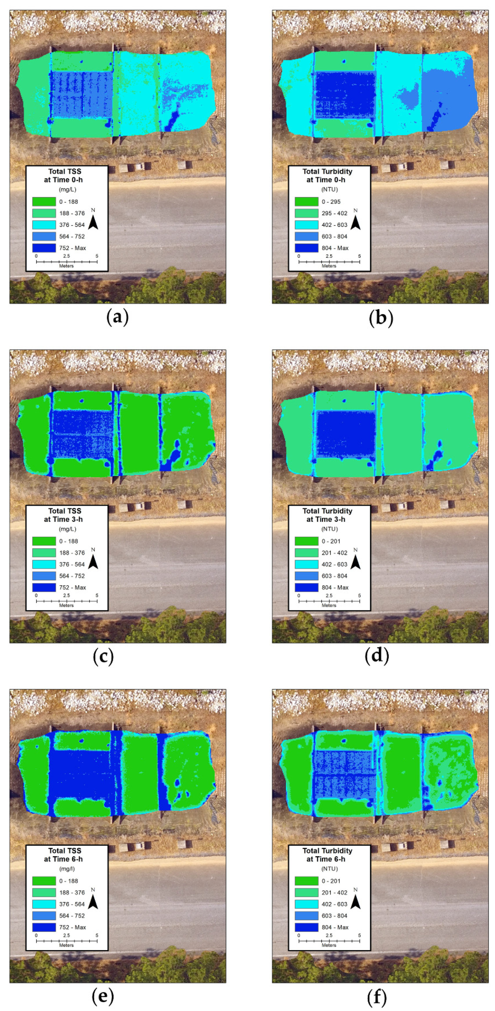
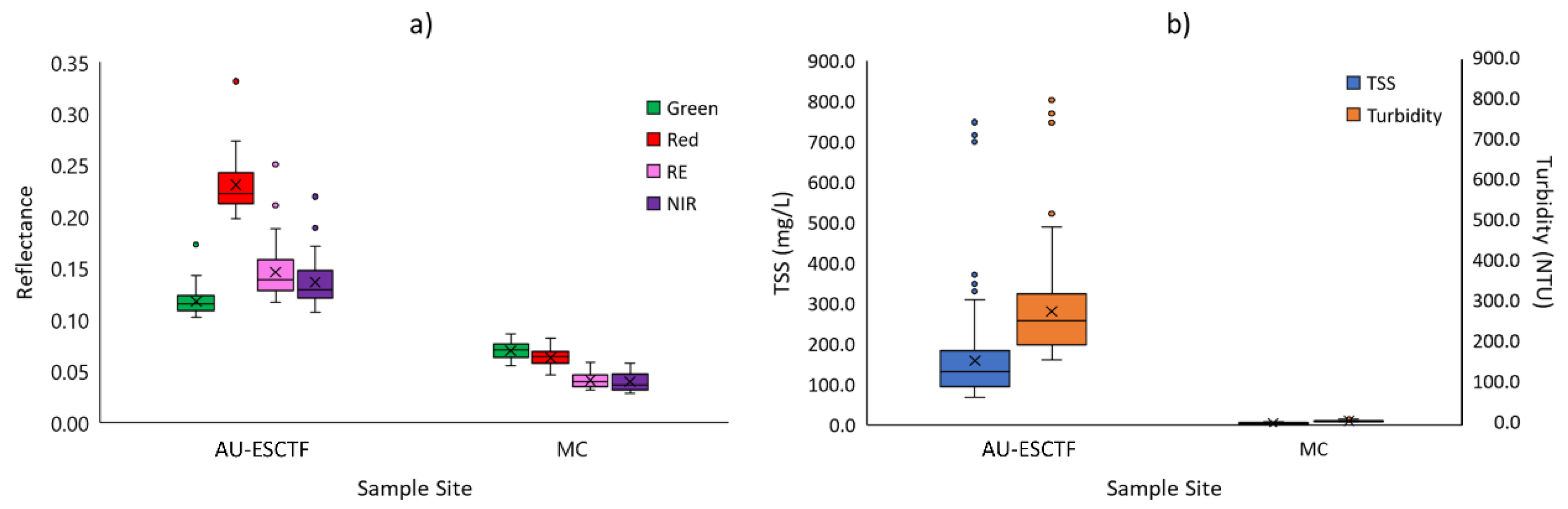
3.1. Turbidity and TSS

Turbidity and TSS results show the settling of particles over the six-h time period and also throughout the water column (Figure 2). The TSS results (Figure 2a) showed a slightly more rapid decline at the beginning and flatten out towards the end compared to turbidity (Figure 2b). This can also be seen in the graphs showing space and time (Figure 2c,d). The first few measurements in the water column closest to the inlet were similar, but rapidly diverge, indicating settlement over time. The first measurement in the water column furthest from the inlet was much lower than the initial measurement in the first water column. This is due to larger solids settling quickly upon entry into the basin, resulting in higher measurements near the front of the basin. The water column was more uniform near the outlet, demonstrating that TSS and turbidity reached equilibrium towards the rear of the sediment basin.

Table 2. Band and water quality measurements shaded to indicate percentile relative to full dataset.

Sampling Location Closest to the Inlet
Time (h)	Green	Red	RE	NIR	TSS Surface (mg/L)	Turbidity Surface (NTU)	TSS Middle (mg/L)	Turbidity Middle (NTU)	TSS Bottom (mg/L)	Turbidity Bottom (NTU)
0.25	0.1067	0.2428	0.2503	0.2193	748.4	803.78	716.8	746.55	699.6	769.65
0.75	0.1274	0.2648	0.1880	0.1714	278.4	417.38	309.2	441.53	329.2	522.38
1.00	0.1275	0.2595	0.1858	0.1708	225.6	392.70	250.8	391.13	294.0	442.58
1.25	0.1162	0.2407	0.1632	0.1505	175.2	379.58	228.0	374.33	232.4	411.60
1.50	0.1141	0.2355	0.1608	0.1514	204.4	315.00	208.8	333.90	212.8	373.80
1.75	0.1071	0.2196	0.1434	0.1310	172.8	295.58	190.8	319.20	212.4	352.80
2.00	0.1157	0.2293	0.1497	0.1401	155.6	284.55	184.4	322.88	201.6	347.55
2.25	0.1146	0.2235	0.1439	0.1388	143.2	270.90	178.0	307.13	188.8	345.45
2.50	0.1123	0.2198	0.1422	0.1312	128.0	253.58	163.2	281.93	187.2	358.05
2.75	0.1071	0.2055	0.1341	0.1273	102.0	233.10	158.8	287.18	162.0	353.85
3.00	0.1079	0.2069	0.1309	0.1230	110.0	217.35	142.8	270.38	178.0	323.93
3.25	0.1023	0.1980	0.1268	0.1222	98.0	206.64	130.4	250.95	170.0	302.93
3.50	0.1058	0.2082	0.1293	0.1270	86.8	193.04	106.4	260.40	168.8	308.18
3.75	0.1084	0.2143	0.1323	0.1294	85.2	186.17	134.0	250.43	158.0	318.15
4.00	0.1066	0.2137	0.1293	0.1268	66.4	171.36	129.6	254.63	137.6	301.88
4.75	0.1427	0.2729	0.1787	0.1503	78.0	162.28	112.8	225.75	141.6	266.70
5.00	0.1055	0.2089	0.1276	0.1182	77.6	163.96	110.4	215.78	144.0	273.00
5.50	0.1231	0.2352	0.1386	0.1370	73.6	169.42	105.2	215.25	136.0	260.93
5.75	0.1152	0.2465	0.1393	0.1364	72.4	161.12	101.2	209.58	133.2	269.33
6.00	0.1200	0.2020	0.1271	0.1201	68.0	169.58	101.6	195.72	128.4	270.38
Sampling Location Furthest from the Inlet
Time (h)	Green	Red	RE	NIR	TSS Surface (mg/L)	Turbidity Surface (NTU)	TSS Middle (mg/L)	Turbidity Middle (NTU)	TSS Bottom (mg/L)	Turbidity Bottom (NTU)
0.25	0.1215	0.2659	0.2111	0.1888	296.8	399.00	371.2	486.68	348.4	488.00
0.75	0.1259	0.2669	0.1716	0.1588	182.4	322.35	244.8	404.78	270.0	405.60
1.00	0.1297	0.2631	0.1694	0.1575	164.0	277.73	218.4	364.35	225.6	348.80
1.25	0.1154	0.2335	0.1402	0.1287	135.2	267.75	189.2	343.35	209.6	340.00
1.50	0.1157	0.2363	0.1488	0.1404	130.4	246.75	162.8	300.83	186.8	317.20
1.75	0.1097	0.2174	0.1345	0.1236	125.6	251.48	142.4	270.90	182.8	322.00
2.00	0.1161	0.2260	0.1393	0.1303	117.6	224.70	132.0	254.10	165.6	299.60
2.25	0.1169	0.2240	0.1391	0.1354	114.8	240.45	114.0	241.50	153.2	309.60
2.50	0.1161	0.2204	0.1318	0.1229	104.0	218.40	112.8	217.88	142.0	278.80
2.75	0.1142	0.2188	0.1287	0.1188	86.8	206.59	104.0	217.88	127.6	268.00
3.00	0.1100	0.2052	0.1238	0.1162	84.8	211.37	100.0	202.65	117.2	229.60
3.25	0.1056	0.2041	0.1205	0.1125	94.8	191.99	101.2	197.66	104.8	209.20
3.50	0.1105	0.2165	0.1252	0.1172	82.4	183.02	98.0	198.35	102.8	224.40
3.75	0.1114	0.2125	0.1248	0.1189	80.4	195.98	95.6	202.97	100.0	213.20
4.00	0.1101	0.2132	0.1203	0.1137	90.0	185.69	92.4	179.81	95.2	200.00
4.25	0.1725	0.3314	0.1628	0.1636	82.4	187.32	87.6	194.46	84.4	191.60
5.00	0.1098	0.2090	0.1163	0.1070	78.0	177.40	89.2	181.76	83.2	186.80
5.50	0.1271	0.2303	0.1266	0.1183	76.0	183.02	80.4	174.62	83.2	186.80
5.75	0.1295	0.2630	0.1432	0.1274	71.2	167.84	78.8	170.73	79.6	178.00
6.00	0.1385	0.2136	0.1319	0.1241	70.0	161.39	78.4	170.10	78.4	170.00
	0th percentile                                                             100th percentile

shows the progressive decrease in suspended sediment through TSS and turbidity measurements along with the response of single-band spectral data at the two sampling locations in the basin. From Table 2, a decreased spectral reflectance can be seen over time as turbidity and TSS decreases. This was expected since there were fewer particles suspended to reflect light at lower TSS levels [30,43,44]. Additionally, Table 2 shows that the red band had consistently higher reflectance compared to the other bands. This was also expected since relatively high concentrations of sediment were present during this study. Water with high levels of suspended sediment has been found to exhibit higher reflectances in all wavelengths, especially in the red and NIR channels [45,46].

3.2. Regression Model Development

The initial analysis was conducted with TSS and turbidity values from all sampling locations. The first set of models considered all water column measurements, while the second set of models considered the water column averages. By testing the correlations between multispectral parameters versus turbidity and TSS, the four single bands and/or band ratios with the highest r values and lowest p values were identified (i.e., band, r and p value rows in Table 2). All possible combinations (ranging from one variable to all four variables) of the selected four bands and/or band ratios were then inputted as predictive variables in a stepwise linear regression procedure. The best r² results were those that included all four variables. Linear regression model coefficients and statistics can be found in

Table 3. Results of correlation analysis and linear regression.

TSS	Band	RE/G	NIR/G	NIR/R	RE/R	Intercept	Sample Size, n	r²	RMSE	RPD	MNB (%)
	r value	0.950	0.932	0.898	0.929	–319.760	60	0.93	30.7	3.6	4.2
	p value	<.0001	<0.0001	<0.0001	<0.0001
	Coefficient	7935.402	–8115.633	15,933.000	–14,837.000
Turbidity	Band	RE/G	NIR/G	NIR/R	RE/R	Intercept	Sample Size, n	r²	RMSE	RPD	MNB (%)
	r value	0.920	0.913	0.874	0.893	–328.016	60	0.85	44.6	2.5	2.9
	p value	<0.0001	<0.0001	<0.0001	<0.0001
	Coefficient	1656.912	–1352.279	2967.325	–2588.921
Averaged TSS	Band	RE/G	NIR/G	NIR/R	RE/R	Intercept	Sample Size, n	r²	RMSE	RPD	MNB (%)
	r value	0.969	0.951	0.916	0.948	–319.775	20	0.97	21.8	5.0	1.5
	p value	<0.0001	<0.0001	<0.0001	<0.0001
	Coefficient	7932.678	–8112.650	15,927.000	–14,831.000
Averaged Turbidity	Band	RE/G	NIR/G	NIR/R	RE/R	Intercept	Sample Size, n	r²	RMSE	RPD	MNB (%)
	r value	0.961	0.953	0.913	0.933	–328.013	20	0.93	30.9	3.5	1.2
	p value	<0.0001	<0.0001	<0.0001	<0.0001
	Coefficient	1657.235	–1352.618	2968.020	–2589.587

. The strongest and most significant correlations were all with band ratios and were consistent between models. Turbidity models had lower r² values than corresponding TSS models due to the lower r values of NIR/R and RE/R. Turbidity r values for NIR/R and RE/R increased to greater than 0.9 when averaged values were used. These findings were reinforced by linear regression values and comparisons of modeled predictions and measurements (Figure 3). In Figure 3, the linear fit is consistent across a wide range of measurements with the mid-water column measurements tending to be closest to the linear fit. Sediment maps were generated by applying the models to the entire sediment basin. Sediment maps using the average TSS and turbidity models were applied at various times to the sediment basin area (Figure 4). Sediment maps using the total TSS and turbidity models were applied at various times to the sediment basin area (Figure 5). Note that the blue rectangle in each map is the lamella plate settler and the blue shading that perpendicularly transects the sediment basin is three rows of wire backed coir baffles attached to metal posts dividing the basin into four sections. Lastly, reflectance values along with TSS and turbidity measurements from this study and from Prior et al. [32] were compared (Figure 6).

4. Discussion

From Table 2, there was a general increase in spectral reflectance with increased TSS and turbidity. The red band was consistently the highest while the green band was consistently the lowest (Table 2 and Figure 6). Red and NIR bands should have the highest spectral response with high suspended sediment concentrations partnered with dampened response from the other spectral bands; these results agree with several other studies comparing sediment concentrations to spectral data [43,44,45,46,47]. From Figure 2, it should be noted that the second sampling location reached equilibrium within the time of sampling, thus allowing for the water column to be homogenous. Conversely, the first sampling location, closest to the inlet, still had varying TSS and turbidity measurements within the water column. Despite these discrepancies, the models were able to produce high r² values, suggesting that water column status does not affect reflectance, at least with high concentrations. This finding is reinforced by comparison between the generated models for average values and for all values. The bands and coefficients for all values versus averaged values models were very similar (Table 3) and the generated maps from these models are almost identical (Figure 4 and Figure 5). Water column status is potentially accounted for more holistically in the averaged models, thus resulting in better model statistics (Table 3).

The models in Table 3, show that the use of multiple band ratios produced higher r² values versus single bands; this was expected since multiple band ratios have been shown to reduce the effect of sun glint from the water’s surface on recorded reflectance [30,47,48]. The models exhibited more significance with red and NIR bands. Averaging water measurements only substantially increases the turbidity r² and r values for NIR/R and RE/R. Overall, r², RMSE, and RPD agree closely as to which models perform well. Generally, RPD > 2 indicates a reliable model [49]. MNB indicated that the models tend to overpredict, with the TSS model being the highest. The generated sediment maps (Figure 4 and Figure 5) show the expected decrease in suspended sediments over time. The resulting maps also looked identical since generated models have similar coefficients (Table 2). This can be excepted since the high levels of suspended solids were consistent throughout the water column, thus resulting in similar models.

In contrast, Prior et al. [32] showed that separate models were required to relate sUAS multispectral imagery to TSS for cases with low and high sediment loads due to stream flow variation. Even with elevated suspended sediment levels present during high flow events, the models still struggled, likely due to influence from stream bed reflectance. The results from the current sediment basin study suggest that the relationship between reflectance and suspended sediment will reach linearity when the bed is not visible due to either excessive cloudiness and or if the depth obscures the bed. The linear regression approach probably produced stronger models than in Prior et al. [32] since a much wider range of suspended sediment values were collected (Figure 6). This wide range of values was much easier to achieve since the sediment basin allowed for continuous sampling over six hours of settlement, whereas stream suspended sediment load is heavily dependent on rainfall and watershed size.

One of the main challenges of this study was syncing of the automatic water samplers among each other and with the sUAS flight. Another challenge was connecting the sUAS to the multispectral sensor within the 15-min break between sampling. Since the plan was to conduct samplings every 15 min for six hours, there should have been 24 samplings. However, only 20 successful samplings were collected due to difficulty in connecting the multispectral sensor and the overheating of the sUAS. Moreover, it should be noted that the automatic samplers purged the intake tubes each time before sampling, causing air bubbles to rise through the water column. This could have affected the settlement of particles and may be the source of the small inflections toward the end of sampling seen in Figure 2. Timing the launch of the sUAS before the purge of the intake tubes was also difficult, thus sUAS imagery during purging could have skewed some results due to the presence of air bubbles at the surface in some instances. Despite these uncertainties, settlement of solids followed an overall expected trend, and stepwise linear regression was able to produce models that could be used for TSS and turbidity predictions.

Several challenges might be faced when implementing sUAS multispectral suspended sediment monitoring for management applications. The most important aspect of sUAS utilization is maintaining a safe environment. This could be difficult to achieve if a sUAS is being used on a construction site. Maintaining a safe launch and landing zone, ensuring line of site visibility as well as keeping a safe distance from obstacles could prove to be difficult on a construction site. Sensor calibration would need to occur prior to every flight as well as ensuring that no shadows are being cast on the sediment basin. Flights are best conducted on overcast days, usually during midmorning, to reduce the potential sun glint off the water surfaces. Hazardous weather, including rain and high wind speeds, should be avoided. Standards and best practices would need to be established and accepted by industry and academia as well as federal and state governments in order to ensure legitimate compliance through sUAS multispectral remote sensing.

Results of this study show that sUAS multispectral imagery could be alternatively used for TSS and turbidity monitoring instead of relying on grab samples. Future studies could improve these results by conducting multiple sediment basin tests with the same soil type to ensure consistent results. Additional tests with different soil types could result in varying spectral reflectance responses, if soil types and/or grain sizes reflect differently. Incorporating sampling depth in tests with lower suspended sediment concentrations could also be beneficial to determine the influence of bed reflectance on sUAS multispectral measurements.

5. Conclusions

This study indicates that sUAS multispectral imagery and linear regression modeling can determine elevated levels of TSS and turbidity with high accuracy in a sediment basin. The measured spectral reflectance showed an expected increase with higher levels of TSS and turbidity in addition to the red and NIR bands increasing the most. Developed models were able to measure a wide range of TSS and turbidity levels while also accounting for both homogeneous and heterogenous water column states. Only the turbidity model that considered all measurements had an r² value below 0.9. The turbidity model that averaged water column values had slightly increased individual band ratio r values and an over increased r² value above 0.9.

This study showed that depth and bed reflectance did not need to be accounted for with elevated TSS and turbidity levels. Future studies should include multiple sediment basin experiments for validation and correlation assurance. Additionally, future studies could include determining when depth and bed reflectance need to be considered and if various soil types and compositions reflect differently when in suspension. This study exhibits the potential for using sUAS technology to assess, measure and monitor sediment basins after high flow events. Further studies are needed to establish monitoring protocols and to investigate if sUAS technology can be used on streams receiving construction and municipal discharges during high flow events.

References

1. Duda, A.M. Addressing nonpoint sources of water pollution must become an international priority. Water Sci. Technol. 1993, 28, 1–11. [Google Scholar] [CrossRef]
2. NRCS. Urban Technical Note No. 1, Erosion and Sedimentation on Construction Sites. Agriculture. In Natural Resources Conservation Service Soil Quality; United States Department of Agriculture: Auburn, AL, USA, 2006. [Google Scholar]
3. Rabení, C.; Jacobson, R.B. Warmwater Streams. In Inland Fisheries Management in North America; American Fisheries Society: Bethesda, MD, USA, 1999; pp. 505–528. [Google Scholar]
4. USEPA. Construction Site Runoff Control Measure. In United States Environmental Protection Agency Stormwater Phase II Finale Rule; EPA Federal Register: Washington, DC, USA, 2005; Volume 833-F-00-008. [Google Scholar]
5. Burton, G.; Gunnison, D.; Lanza, G.R. Survival of pathogenic bacteria in various freshwater sediments. Appl. Environ. Microbiol. 1987, 53, 633–638. [Google Scholar] [CrossRef] [PubMed] [Green Version]
6. Mitsch, W.J.; Reeder, B.C. Nutrient and hydrologic budgets of a Great Lakes coastal freshwater wetland during a drought year. Wetl. Ecol. Manag. 1992, 1, 211–222. [Google Scholar] [CrossRef]
7. Wohl, E.; Bledsoe, B.P.; Jacobson, R.B.; Poff, N.L.; Rathburn, S.L.; Walters, D.M.; Wilcox, A.C. The natural sediment regime in rivers: Broadening the foundation for ecosystem management. BioScience 2015, 65, 358–371. [Google Scholar] [CrossRef] [Green Version]
8. Lake, P.S.; Palmer, M.A.; Biro, P.; Cole, J.; Covich, A.P.; Dahm, C.; Gibert, J.; Goedkoop, W.; Martens, K.; Verhoeven, J. Global Change and the Biodiversity of Freshwater Ecosystems: Impacts on Linkages between Above-Sediment and Sediment Biota: All forms of anthropogenic disturbance—changes in land use, biogeochemical processes, or biotic addition or loss—not only damage the biota of freshwater sediments but also disrupt the linkages between above-sediment and sediment-dwelling biota. BioScience 2000, 50, 1099–1107. [Google Scholar]
9. Pimentel, D.; Kounang, N. Ecology of soil erosion in ecosystems. Ecosystems 1998, 1, 416–426. [Google Scholar] [CrossRef]
10. Walker, W.J.; McNutt, R.P.; Maslanka, C.K. The potential contribution of urban runoff to surface sediments of the Passaic River: Sources and chemical characteristics. Chemosphere 1999, 38, 363–377. [Google Scholar] [CrossRef]
11. USEPA. United States Environmental Protection Agency National Pollutant Discharge Elimination System (NPDES); EPA Federal Register: Washington, DC, USA, 2010.
12. USEPA. United States Environmental Protection Agency Construction General Permit (CGP)—Fact Sheet; EPA Federal Register: Washington, DC, USA, 2012.
13. Perez, M.A.; Zech, W.C.; Vasconcelos, J.G.; Fang, X. Large-Scale Performance Testing of Temporary Sediment Basin Treatments and High-Rate Lamella Settlers. Water 2019, 11, 316. [Google Scholar] [CrossRef] [Green Version]
14. Perez, M.A.; Zech, W.C.; Donald, W.N.; Turochy, R.; Fagan, B.G. Transferring Innovative Erosion and Sediment Control Research Results into Industry Practice. Water 2019, 11, 2549. [Google Scholar] [CrossRef] [Green Version]
15. Fang, X.; Zech, W.; Logan, C. Stormwater field evaluation and its challenges of a sediment basin with skimmer and baffles at a highway construction site. Water 2015, 7, 3407–3430. [Google Scholar] [CrossRef]
16. Zech, W.; Logan, C.; Fang, X. State of the practice: Evaluation of sediment basin design, construction, maintenance, and inspection procedures. Pract. Period. Struct. Des. Constr. 2014, 19, 04014006. [Google Scholar] [CrossRef] [Green Version]
17. USEPA. Turbidity and Total Solids. In United States Environmental Protection Agency Voluntary Estuary Monitoring Manual; USEPA Office of Wetlands, Oceans, and Watersheds: Washington, DC, USA, 2006; Volume EPA-842-B-06-003. [Google Scholar]
18. Tomsett, C.; Leyland, J. Remote sensing of river corridors: A review of current trends and future directions. River Res. Appl. 2019. [Google Scholar] [CrossRef]
19. Umar, M.; Rhoads, B.L.; Greenberg, J.A. Use of multispectral satellite remote sensing to assess mixing of suspended sediment downstream of large river confluences. J. Hydrol. 2018, 556, 325–338. [Google Scholar] [CrossRef]
20. Becker, R.H.; Sayers, M.; Dehm, D.; Shuchman, R.; Quintero, K.; Bosse, K.; Sawtell, R. Unmanned aerial system based spectroradiometer for monitoring harmful algal blooms: A new paradigm in water quality monitoring. J. Great Lakes Res. 2019, 45, 444–453. [Google Scholar] [CrossRef]
21. Manfreda, S.; McCabe, M.; Miller, P.; Lucas, R.; Pajuelo Madrigal, V.; Mallinis, G.; Ben Dor, E.; Helman, D.; Estes, L.; Ciraolo, G. On the use of unmanned aerial systems for environmental monitoring. Remote Sens. 2018, 10, 641. [Google Scholar] [CrossRef] [Green Version]
22. Nowak, M.M.; Dziób, K.; Bogawski, P. Unmanned Aerial Vehicles (UAVs) in environmental biology: A review. Eur. J. Ecol. 2019, 4, 56–74. [Google Scholar] [CrossRef]
23. Simic Milas, A.; Sousa, J.J.; Warner, T.A.; Teodoro, A.C.; Peres, E.; Gonçalves, J.A.; Delgado Garcia, J.; Bento, R.; Phinn, S.; Woodget, A. Unmanned Aerial Systems (UAS) for environmental applications special issue preface. Int. J. Remote Sens. 2018, 39, 4845–4851. [Google Scholar] [CrossRef]
24. Briggs, M.A.; Dawson, C.B.; Holmquist-Johnson, C.L.; Williams, K.H.; Lane, J.W. Efficient hydrogeological characterization of remote stream corridors using drones. Hydrol. Process. 2018, 33. [Google Scholar] [CrossRef] [Green Version]
25. Fitch, K.; Kelleher, C.; Caldwell, S.; Joyce, I. Airborne thermal infrared videography of stream temperature anomalies from a small unoccupied aerial system. Hydrol. Process. 2018, 32, 2616–2619. [Google Scholar] [CrossRef]
26. Lega, M.; Kosmatka, J.; Ferrara, C.; Russo, F.; Napoli, R.; Persechino, G. Using advanced aerial platforms and infrared thermography to track environmental contamination. Environ. Forensics 2012, 13, 332–338. [Google Scholar] [CrossRef]
27. Lega, M.; Napoli, R.M. Aerial infrared thermography in the surface waters contamination monitoring. Desalin. Water Treat. 2010, 23, 141–151. [Google Scholar] [CrossRef]
28. Su, T.-C. A study of a matching pixel by pixel (MPP) algorithm to establish an empirical model of water quality mapping, as based on unmanned aerial vehicle (UAV) images. Int. J. Appl. Earth Obs. Geoinf. 2017, 58, 213–224. [Google Scholar] [CrossRef]
29. Vogt, M.C.; Vogt, M.E. Near-remote sensing of water turbidity using small unmanned aircraft systems. Environ. Pract. 2016, 18, 18–31. [Google Scholar] [CrossRef]
30. Larson, M.D.; Simic Milas, A.; Vincent, R.K.; Evans, J.E. Multi-depth suspended sediment estimation using high-resolution remote-sensing UAV in Maumee River, Ohio. Int. J. Remote Sens. 2018, 39, 5472–5489. [Google Scholar] [CrossRef]
31. Ehmann, K.; Kelleher, C.; Condon, L.E. Monitoring turbidity from above: Deploying small unoccupied aerial vehicles to image in-stream turbidity. Hydrol. Process. 2019, 33, 1013–1021. [Google Scholar] [CrossRef]
32. Prior, E.M.; O’Donnell, F.C.; Brodbeck, C.; Runion, G.B.; Shepherd, S.L. Investigating small unoccupied aerial systems (sUAS) multispectral imagery for total suspended solids and turbidity monitoring in small streams. Int. J. Remote Sens. 2020, 1–26. [Google Scholar] [CrossRef]
33. Perez, M.; Zech, W.; Fang, X.; Vasconcelos, J. Methodology and development of a large-scale sediment basin for performance testing. J. Irrig. Drain. Eng. 2016, 142, 04016042. [Google Scholar] [CrossRef]
34. Poncet, A.M.; Knappenberger, T.; Brodbeck, C.; Fogle, M.; Shaw, J.N.; Ortiz, B.V. Multispectral UAS Data Accuracy for Different Radiometric Calibration Methods. Remote Sens. 2019, 11, 1917. [Google Scholar] [CrossRef] [Green Version]
35. DJI. DJI Phantom 4 Specs. Available online: https://www.dji.com/phantom-4/info#downloads (accessed on 8 December 2019).
36. Datasheet: The Multi-Band Sensor Designed for Agriculture. Available online: https://tecnitop.com/wp-content/uploads/2015/10/Sequoia_Datasheet.pdf (accessed on 3 May 2020).
37. Gauci, A.A.; Brodbeck, C.J.; Poncet, A.M.; Knappenberger, T. Assessing the Geospatial Accuracy of Aerial Imagery Collected with Various UAS Platforms. Am. Soc. Agric. Biol. Eng. 2018. [Google Scholar] [CrossRef]
38. USEPA. Method 160.2: Nonfilterable (Suspended Solids), Water. In United States Environmental Protection Agency Standard Operating Procedure for the Analysis of Residue; EPA Federal Register: Washington, DC, USA, 1971. [Google Scholar]
39. USEPA. Method 180.1: Determination of Turbidity by Nephelometry. In United States Environmental Protection Agency; EPA Federal Register: Washington, DC, USA, 1993. [Google Scholar]
40. Iqbal, F.; Lucieer, A.; Barry, K. Simplified radiometric calibration for UAS-mounted multispectral sensor. Eur. J. Remote Sens. 2018, 51, 301–313. [Google Scholar] [CrossRef]
41. SAS Institute Inc. SAS User’s Guide: Basics; SAS: Cary, NC, USA, 1982; p. 923. [Google Scholar]
42. SAS Institute Inc. SAS User’s Guide: Statistics; SAS: Cary, NC, USA, 1985; p. 956. [Google Scholar]
43. Lodhi, M.A.; Rundquist, D.C.; Han, L.; Kuzila, M.S. Estimation of suspended sediment concentration in water using integrated surface reflectance. Geocarto Int. 1998, 13, 11–15. [Google Scholar] [CrossRef]
44. Shen, F.; Suhyb Salama, M.; Zhou, Y.-X.; Li, J.-F.; Su, Z.; Kuang, D.-B. Remote-sensing reflectance characteristics of highly turbid estuarine waters—A comparative experiment of the Yangtze River and the Yellow River. Int. J. Remote Sens. 2010, 31, 2639–2654. [Google Scholar] [CrossRef]
45. Doxaran, D.; Froidefond, J.-M.; Castaing, P. Remote-sensing reflectance of turbid sediment-dominated waters. Reduction of sediment type variations and changing illumination conditions effects by use of reflectance ratios. Appl. Opt. 2003, 42, 2623–2634. [Google Scholar] [CrossRef] [PubMed]
46. Sokoletsky, L.; Fang, S.; Yang, X.; Wei, X. Evaluation of empirical and semianalytical spectral reflectance models for surface suspended sediment concentration in the highly variable estuarine and coastal waters of East China. IEEE J. Sel. Top. Appl. Earth Obs. Remote Sens. 2016, 9, 5182–5192. [Google Scholar] [CrossRef]
47. Pereira, L.S.; Andes, L.C.; Cox, A.L.; Ghulam, A. Measuring Suspended-Sediment Concentration and Turbidity in the Middle Mississippi and Lower Missouri Rivers Using Landsat Data. JAWRA J. Am. Water Resour. Assoc. 2018, 54, 440–450. [Google Scholar] [CrossRef]
48. Chen, Z.; Hu, C.; Muller-Karger, F. Monitoring turbidity in Tampa Bay using MODIS/Aqua 250-m imagery. Remote Sens. Environ. 2007, 109, 207–220. [Google Scholar] [CrossRef]
49. Chang, C.-W.; Laird, D.A.; Mausbach, M.J.; Hurburgh, C.R. Near-infrared reflectance spectroscopy–principal components regression analyses of soil properties. Soil Sci. Soc. Am. J. 2001, 65, 480–490. [Google Scholar] [CrossRef] [Green Version]
Figure 1. Map of the Auburn University Erosion and Sediment Control Testing Facility sediment basin where the experiment was conducted. The sampling locations, ground control points for spatially referencing the drone flights and the outlet of the sediment basin are shown.
Drones 04 00054 g001
Figure 2. TSS and turbidity from the Auburn University Erosion and Sediment Control Testing Facility (AU-ESCTF): (a) averaged TSS of water column from the two sampling locations over time, (b) averaged turbidity of water column from the two sampling locations over time, (c) TSS over time and space with 0 m being furthest upstream and closest to the inlet, (d) turbidity over time and space with 0 m being furthest upstream and closest to the inlet.
Drones 04 00054 g002
Figure 3. Scatter plots of measured TSS and turbidity compared to modeled results: (a) all TSS values and modeled TSS values, (b) all turbidity values and modeled turbidity values, (c) averaged water column TSS values and modeled averaged water column TSS values, (d) averaged water column turbidity values and modeled averaged water column turbidity values.
Drones 04 00054 g003
Figure 4. Generated sUAS average TSS and turbidity maps (blue rectangle is the lamella plate settler): (a) average TSS map at time equals 0 h, (b) average turbidity map at time equals 0 h, (c) average TSS map at time equals 3 h, (d) average turbidity map at time equals 3 h, (e) average TSS map at time equals 6 h, (f) average turbidity map at time equals 6 h.
Drones 04 00054 g004
Figure 5. Generated sUAS total TSS and turbidity maps (blue rectangle is the lamella plate settler): (a) total TSS map at time equals 0 h, (b) total turbidity map at time equals 0 h, (c) total TSS map at time equals 3 h, (d) total turbidity map at time equals 3 h, (e) total TSS map at time equals 6 h, (f) total turbidity map at time equals 6 h.
Drones 04 00054 g005
Figure 6. Comparison of results to Prior et al. [32]: (a) box and whisker plots of reflectance values from this study (AU-ESCTF) and from Prior et al. [32] sampling at Moores Creek, Lanett, AL, USA (MC), (b) box and whisker plots of TSS and turbidity from this study (AUESCTF) and from Prior et al. [32] sampling at Moores Creek, Lanett, AL, USA (MC).
Drones 04 00054 g006