Measures of Canopy Structure from Low-Cost UAS for Monitoring Crop Nutrient Status

 ,
,  ,
,  ,
, 
Abstract
1. Introduction
2. Materials and Methods
2.1. Study Site
2.2. Data Collection
2.3. Data Processing
2.4. Canopy Surface Analysis
2.5. Visible Band Spectral Metrics
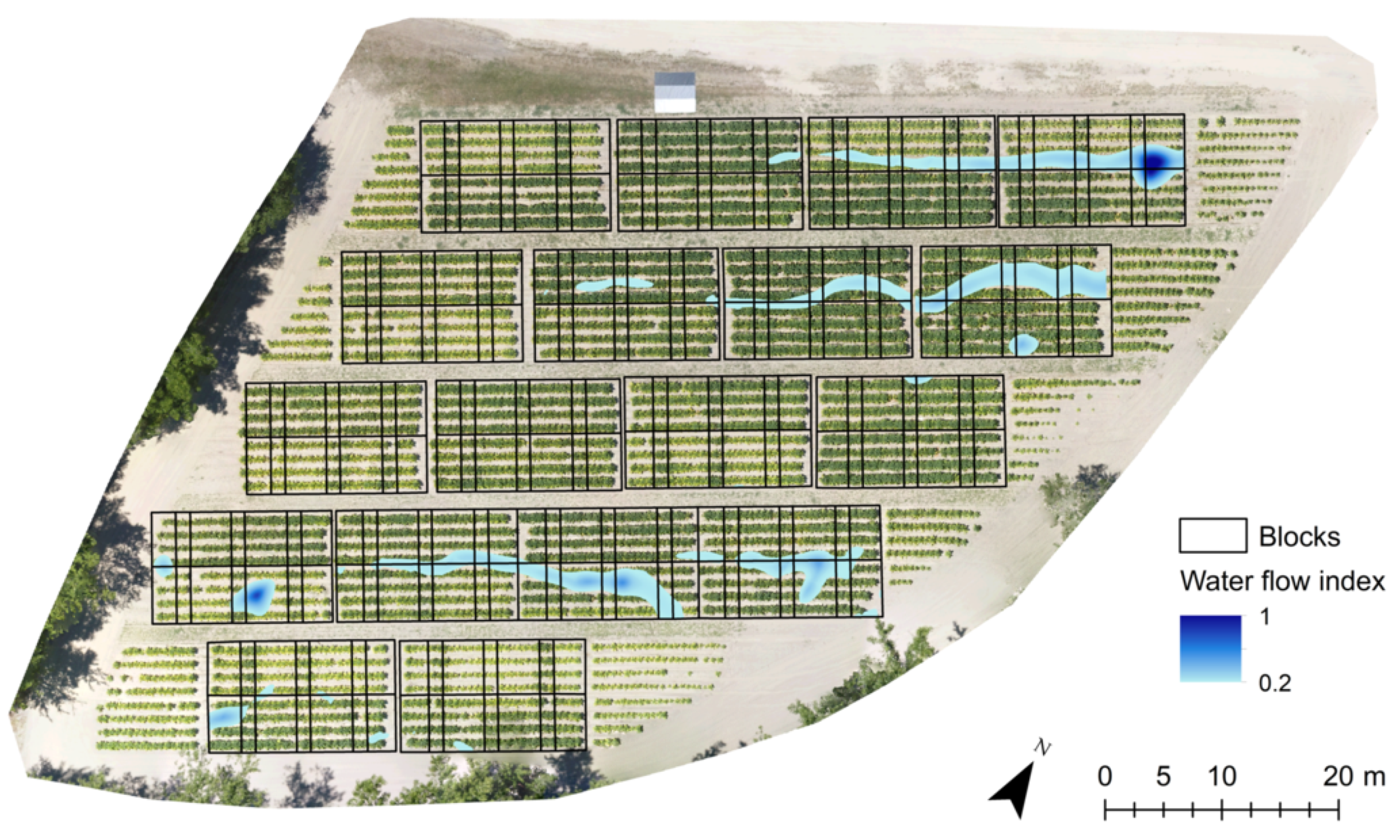
2.6. Water Flow Index
2.7. Statistics
3. Results
3.1. Foliar Nutrient Concentrations
3.2. UAS-Derived Canopy Metrics
3.2.1. Mean Crop Height
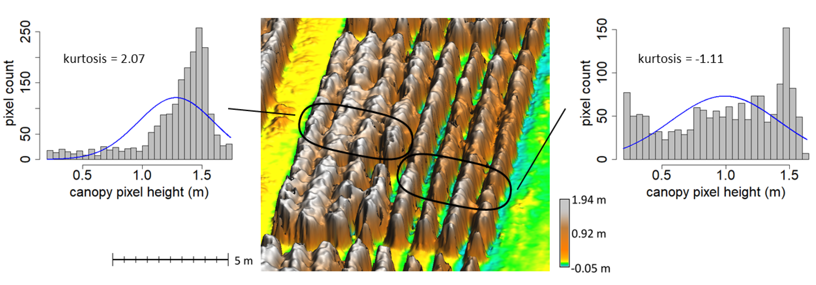
3.2.2. Crop Height Histogram Kurtosis
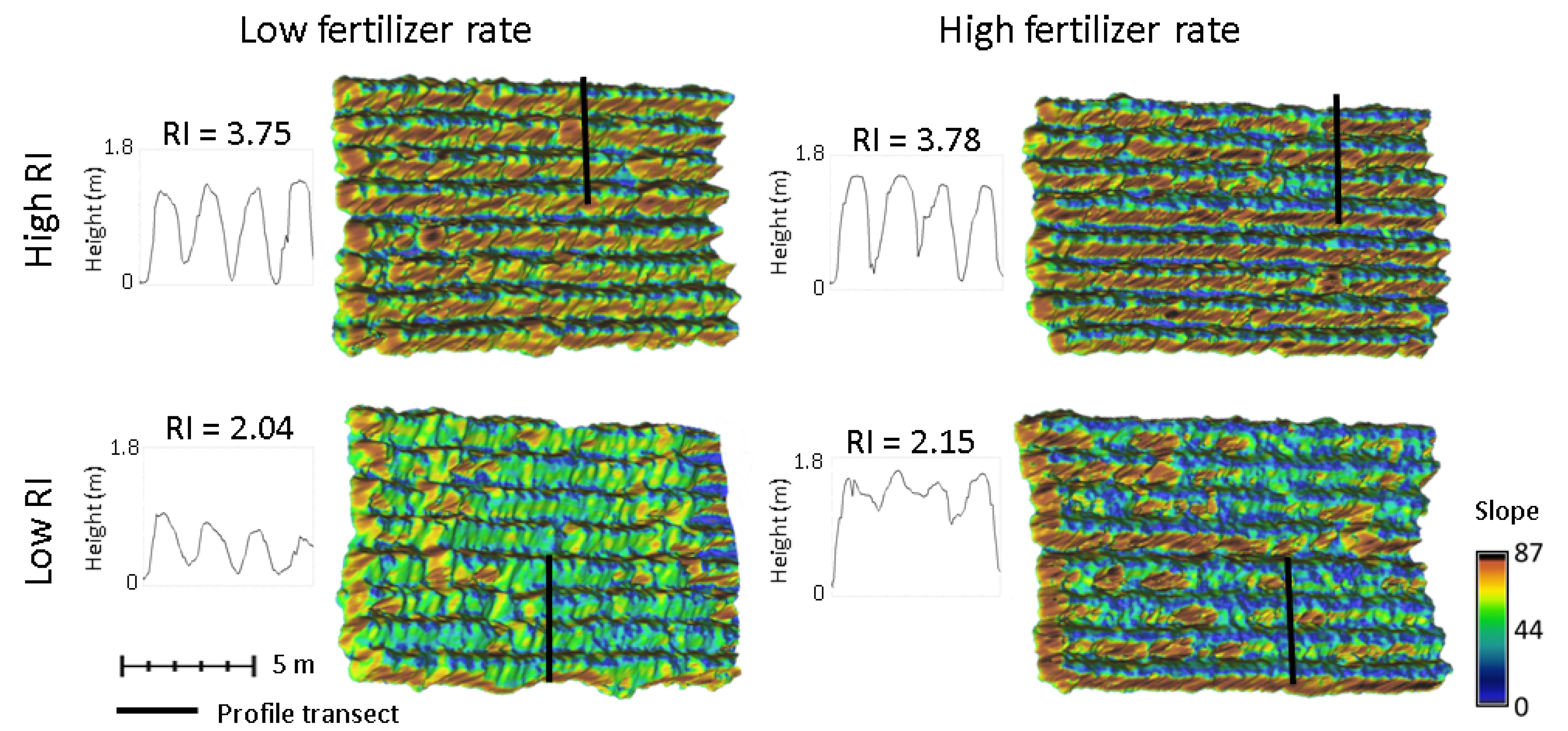
3.2.3. Rumple Index
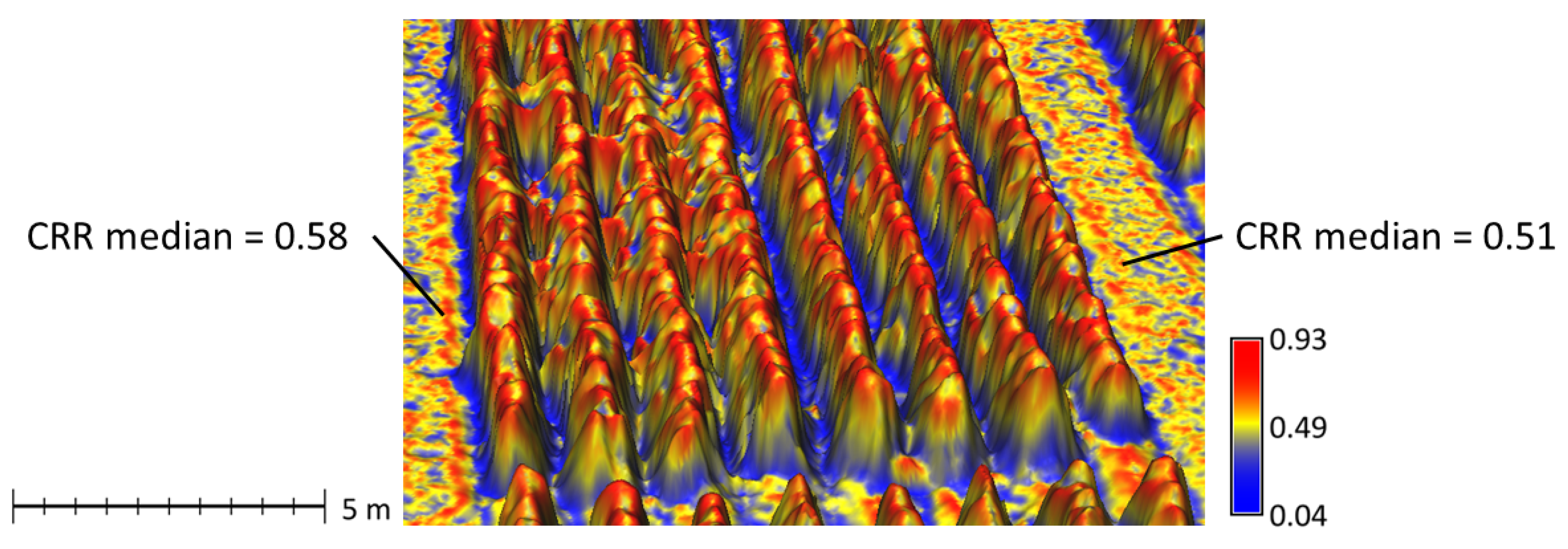
3.2.4. Canopy Relief Ratio
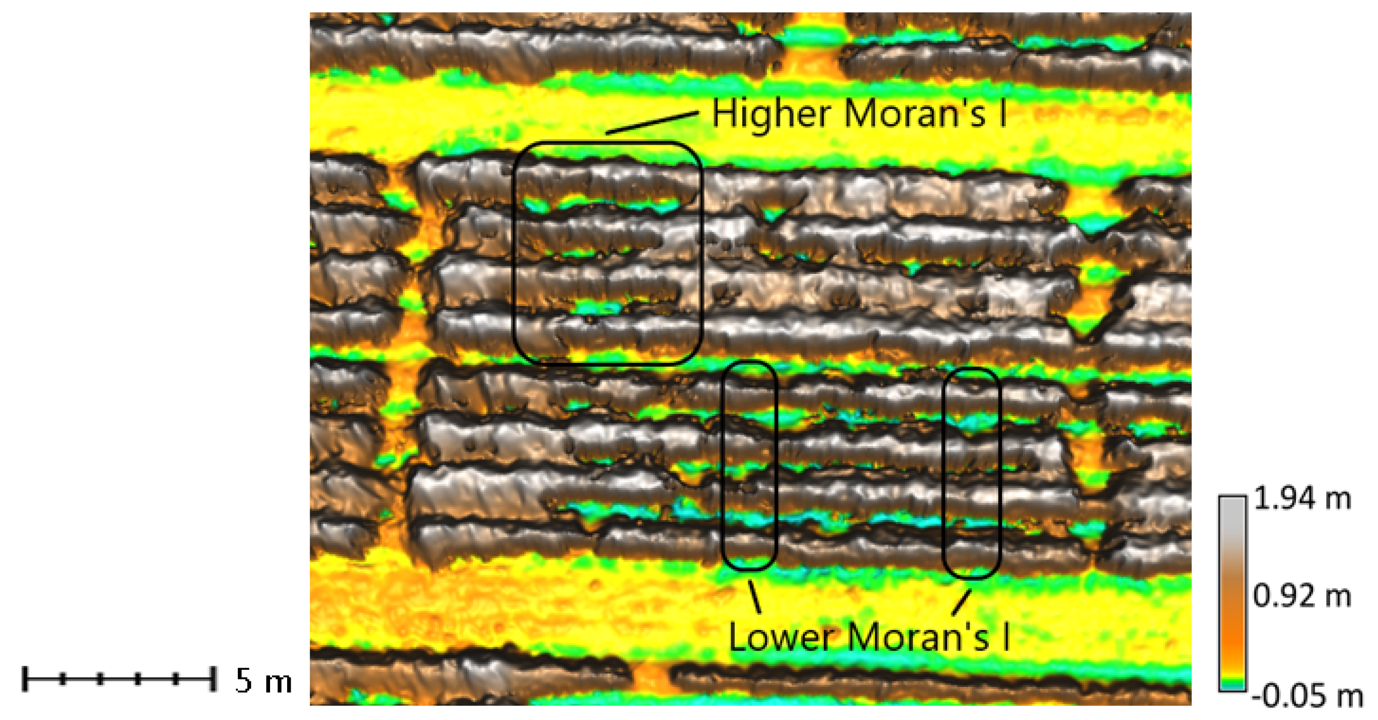
3.2.5. Spatial Autocorrelation of Crop Height
3.2.6. Water Flow Index
3.2.7. Triangular Greenness Index
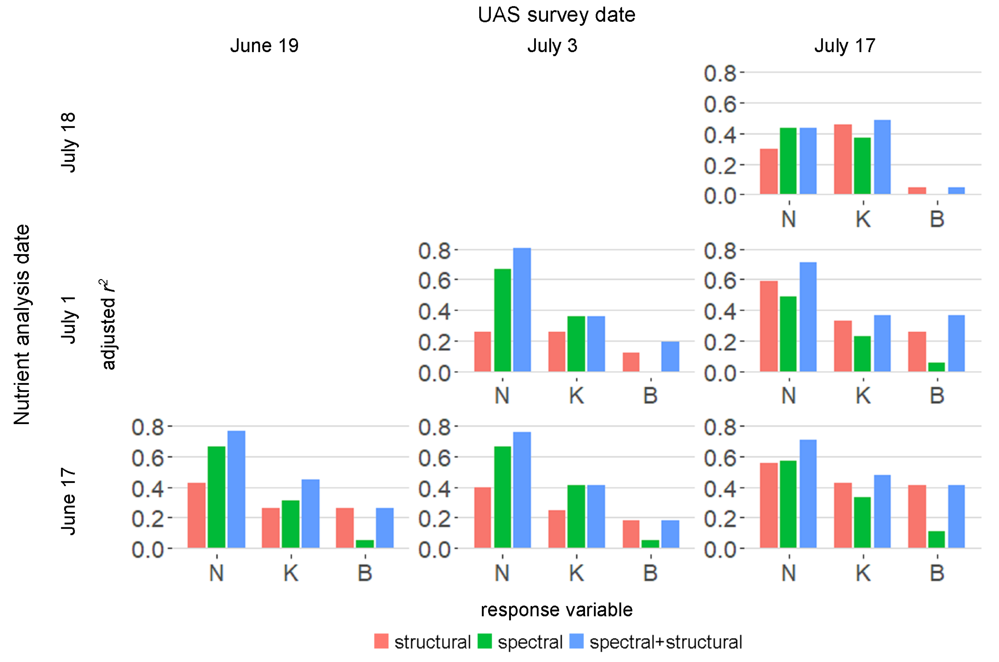
3.3. Overall Relationship between the Crop Canopy Shape, Reflectance, and Nutrient Concentration
3.3.1. Nitrogen
3.3.2. Potassium
3.3.3. Boron
4. Discussion
5. Conclusions
Author Contributions
Funding
Acknowledgments
Conflicts of Interest
Abbreviations
| UAS | Unmanned aerial system |
| N | Nitrogen |
| P | Phosphorus |
| K | Potassium |
| B | Boron |
| NDVI | Normalized Difference Vegetation Index |
| VARI | Visible Atmospheric Resistance Index |
| TGI | Triangular Greenness Index |
| RGB | Red Green Blue |
| SfM | Structure from Motion |
| LAI | Leaf area index |
| CEC | Cation exchange capacity |
| DSM | Digital surface model |
| DEM | Digital elevation model |
| RMSEz | Root mean squared error in z direction |
| CSM | Crop surface model |
| RI | Rumple index |
| CRR | Canopy relief ratio |
| IQR | Interquartile range |
| VIF | Variable inflation factor |
| AIC | Akaike’s information criteria |
References
- Stafford, J.V. Implementing Precision Agriculture in the 21st Century. J. Agric. Eng. Res. 2000, 76, 267–275. [Google Scholar] [CrossRef]
- Hunt, E.R.; Daughtry, C.S.T. What good are unmanned aircraft systems for agricultural remote sensing and precision agriculture? Int. J. Remote Sens. 2018, 39, 5345–5376. [Google Scholar] [CrossRef]
- Zhang, C.; Kovacs, J. The application of small unmanned aerial systems for precision agriculture: A review. Precis. Agric. 2012, 13, 693–712. [Google Scholar] [CrossRef]
- Corti, M.; Cavalli, D.; Cabassi, G.; Vigoni, A.; Degano, L.; Marino Gallina, P. Application of a low-cost camera on a UAV to estimate maize nitrogen-related variables. Precis. Agric. 2019, 20, 675–696. [Google Scholar] [CrossRef]
- Cilia, C.; Panigada, C.; Rossini, M.; Meroni, M.; Busetto, L.; Amaducci, S.; Boschetti, M.; Picchi, V.; Colombo, R. Nitrogen Status Assessment for Variable Rate Fertilization in Maize through Hyperspectral Imagery. Remote Sens. 2014, 6, 6549–6565. [Google Scholar] [CrossRef]
- Maresma, A.; Lloveras, J.; Martínez-Casasnovas, J.A. Use of Multispectral Airborne Images to Improve In-Season Nitrogen Management, Predict Grain Yield and Estimate Economic Return of Maize in Irrigated High Yielding Environments. Remote Sens. 2018, 10, 543. [Google Scholar] [CrossRef]
- Berger, K.; Verrelst, J.; Féret, J.B.; Wang, Z.; Wocher, M.; Strathmann, M.; Danner, M.; Mauser, W.; Hank, T. Crop nitrogen monitoring: Recent progress and principal developments in the context of imaging spectroscopy missions. Remote Sens. Environ. 2020, 242, 111758. [Google Scholar] [CrossRef]
- Mitra, G. Essential plant nutrients and recent concepts about their uptake. In Essential Plant Nutrients, 1st ed.; Springer: Cham, Switzerland, 2017; pp. 3–36. [Google Scholar] [CrossRef]
- Henry, J.B.; Vann, M.C.; Lewis, R.S. Agronomic Practices Affecting Nicotine Concentration in Flue-Cured Tobacco: A Review. Agron. J. 2019, 111, 3067–3075. [Google Scholar] [CrossRef]
- Ruiz, J.M.; Lopez-Lefebre, L.R.; Sanchez, E.; Rivero, R.M.; Garcia, P.C.; Romero, L. Preliminary studies on the influence of boron on the foliar biomass and quality of tobacco leaves subjected to NO3- fertilisation. J. Sci. Food Agric. 2001, 81, 739–744. [Google Scholar] [CrossRef]
- Tariq, M.; Akbar, A.; Lataf-ul-Haq.; Khan, A. Comparing Application Methods for Boron Fertilizer on the Yield and Quality of Tobacco (Nicotiana tabacum L.). Commun. Soil Sci. Plant Anal. 2010, 41, 1525–1537. [Google Scholar] [CrossRef]
- Römheld, V. Diagnosis of deficiency and toxicity of nutrients. In Marschner’s Mineral Nutrition of Higher Plants; Elsevier Science & Technology: San Diego, CA, USA, 2011. [Google Scholar]
- Stroppiana, D.; Migliazzi, M.; Chiarabini, V.; Crema, A.; Musanti, M.; Franchino, C.; Villa, P. Rice yield estimation using multispectral data from UAV: A preliminary experiment in northern Italy. In Proceedings of the 2015 IEEE International Geoscience and Remote Sensing Symposium (IGARSS), Milan, Italy, 26–31 July 2015; IEEE: Piscataway, NJ, USA, 2015; pp. 4664–4667. [Google Scholar] [CrossRef]
- Bolton, D.K.; Friedl, M.A. Forecasting crop yield using remotely sensed vegetation indices and crop phenology metrics. Agric. For. Meteorol. 2013, 173, 74–84. [Google Scholar] [CrossRef]
- Stanton, C.; Starek, M.J.; Elliott, N.; Brewer, M.; Maeda, M.M.; Chu, T. Unmanned aircraft system-derived crop height and normalized difference vegetation index metrics for sorghum yield and aphid stress assessment. J. Appl. Remote Sens. 2017, 11, 026035. [Google Scholar] [CrossRef]
- Severtson, D.; Callow, N.; Flower, K.; Neuhaus, A.; Olejnik, M.; Nansen, C. Unmanned aerial vehicle canopy reflectance data detects potassium deficiency and green peach aphid susceptibility in canola. Precis. Agric. 2016, 17, 659–677. [Google Scholar] [CrossRef]
- Henry, J.B. Characterization of Tobacco Nutrient Disorders via Remote Sensing. Ph.D. Thesis, North Carolina State University, Raleigh, NC, USA, 2019. [Google Scholar]
- Adão, T.; Hruška, J.; Pádua, L.; Bessa, J.; Peres, E.; Morais, R.; Sousa, J. Hyperspectral Imaging: A Review on UAV-Based Sensors, Data Processing and Applications for Agriculture and Forestry. Remote Sens. 2017, 9, 1110. [Google Scholar] [CrossRef]
- Hunt, E.R.; Doraiswamy, P.C.; McMurtrey, J.E.; Daughtry, C.S.T.; Perry, E.M.; Akhmedov, B. A visible band index for remote sensing leaf chlorophyll content at the canopy scale. Int. J. Appl. Earth Obs. Geoinf. 2013, 21, 103–112. [Google Scholar] [CrossRef]
- Gitelson, A.A.; Kaufman, Y.J.; Stark, R.; Rundquist, D. Novel algorithms for remote estimation of vegetation fraction. Remote Sens. Environ. 2002, 80, 76–87. [Google Scholar] [CrossRef]
- Liew, O.W.; Chong, P.C.J.; Li, B.; Asundi, A.K. Signature Optical Cues: Emerging Technologies for Monitoring Plant Health. Sensors 2008, 8, 3205–3239. [Google Scholar] [CrossRef]
- Carrivick, J.; Smith, M.; Quincey, D. Structure from Motion in the Geosciences, 1st ed.; Number Book, Whole in New Analytical Methods in Earth and Environmental Science; Wiley-Blackwell: Hoboken, NJ, USA, 2016. [Google Scholar]
- Hunt, E.R.; Rondon, S.I. Detection of potato beetle damage using remote sensing from small unmanned aircraft systems. J. Appl. Remote Sens. 2017, 11, 026013. [Google Scholar] [CrossRef]
- Parker, G.G.; Russ, M.E. The canopy surface and stand development: Assessing forest canopy structure and complexity with near-surface altimetry. For. Ecol. Manag. 2004, 189, 307–315. [Google Scholar] [CrossRef]
- Li, W.; Niu, Z.; Chen, H.; Li, D. Characterizing canopy structural complexity for the estimation of maize LAI based on ALS data and UAV stereo images. Int. J. Remote Sens. 2017, 38, 2106–2116. [Google Scholar] [CrossRef]
- Li, W.; Niu, Z.; Chen, H.; Li, D.; Wu, M.; Zhao, W. Remote estimation of canopy height and aboveground biomass of maize using high-resolution stereo images from a low-cost unmanned aerial vehicle system. Ecol. Indic. 2016, 67, 637–648. [Google Scholar] [CrossRef]
- Bendig, J.; Bolten, A.; Bennertz, S.; Broscheit, J.; Eichfuss, S.; Bareth, G. Estimating Biomass of Barley Using Crop Surface Models (CSMs) Derived from UAV-Based RGB Imaging. Remote Sens. 2014, 6, 10395–10412. [Google Scholar] [CrossRef]
- Chu, T.; Chen, R.; Landivar, J.A.; Maeda, M.M.; Yang, C.; Starek, M.J. Cotton growth modeling and assessment using unmanned aircraft system visual-band imagery. J. Appl. Remote Sens. 2016, 10, 036018-17. [Google Scholar] [CrossRef]
- Fisher, L.R. Flue-Cured Tobacco Guide, rev. ed.; North Carolina Cooperative Extension: Raleigh, NC, USA, 2019. [Google Scholar]
- Mitasova, H.; Mitas, L.; Harmon, R.S. Simultaneous spline approximation and topographic analysis for lidar elevation data in open-source GIS. IEEE Geosci. Remote Sens. Lett. 2005, 2, 375–379. [Google Scholar] [CrossRef]
- Mitas, L.; Mitasova, H.; Kosinovsky, I.; McCauley, D.; Hofierka, J.; Zubal, S.; Lacko, M. GRASS GIS: V.surf.rst Module; GRASS: Raleigh, NC, USA, 2018. [Google Scholar]
- North Carolina Geographic Information Coordinating Council. NC OneMap Orthoimagery; North Carolina Geographic Information Coordinating Council: Raleigh, NC, USA, 2017. [Google Scholar]
- North Carolina Emergency Management. NC Floodplain Mapping Program QL2 LiDAR; North Carolina Emergency Management: Raleigh, NC, USA, 2015. [Google Scholar]
- Jensen, J.; Mathews, A. Assessment of image-based point cloud products to generate a bare earth surface and estimate canopy heights in a woodland ecosystem. Remote Sens. 2016, 8, 50. [Google Scholar] [CrossRef]
- Jenness, J.S. Calculating landscape surface area from digital elevation models. Wildl. Soc. Bull. 2004, 32, 829–839. [Google Scholar] [CrossRef]
- Pike, R.J.; Wilson, S.E. Elevation-Relief Ratio, Hypsometric Integral, and Geomorphic Area-Altitude Analysis. Geol. Soc. Am. Bull. 1971, 82, 1079. [Google Scholar] [CrossRef]
- Moran, P.A.P. Notes of continuous stochastic phenomena. Biometrika 1950, 37, 17–23. [Google Scholar] [CrossRef]
- Mitasova, H.; Thaxton, C.; Hofierka, J.; McLaughlin, R.; Moore, A.; Mitas, L. Path sampling method for modeling overland water flow, sediment transport, and short term terrain evolution in Open Source GIS. In Developments in Water Science; Elsevier B.V.: Amsterdam, The Netherlands, 2004; Volume 55, pp. 1479–1490. [Google Scholar] [CrossRef]
- Henry, J.B.; Vann, M.; McCall, I.; Cockson, P.; Whipker, B.E. Nutrient Disorders of Burley and Flue-Cured Tobacco: Part 2—Micronutrient Disorders. Crop. Forage Turfgrass Manag. 2018, 4, 1–7. [Google Scholar] [CrossRef]
- Henry, J.B.; Vann, M.; McCall, I.; Cockson, P.; Whipker, B.E. Nutrient Disorders of Burley and Flue-Cured Tobacco: Part 1—Macronutrient Deficiencies. Crop Forage Turfgrass Manag. 2018, 4, 1–8. [Google Scholar] [CrossRef]
- Raper, C.D.; Smith, W.T. Factors Affecting the Development of Flue-cured Tobacco Grown in Artificial Environments. V. Effects of Humidity and Nitrogen Nutrition1. Agron. J. 1975, 67, 307–312. [Google Scholar] [CrossRef]
- McMurtrey, J.E. Symptoms on Field-Grown Tobacco Characteristic of the Deficient Supply of Each of Several Essential Chemical Elements; Technical Report 612; United States Department of Agriculture: Washington, DC, USA, 1938. [Google Scholar]
- Peterson, B.G.; Carl, P. PerformanceAnalytics: Econometric Tools for Performance and Risk Analysis; CRANE Co.: Stamford, CT, USA, 2020. [Google Scholar]
- Roussel, J.R.; Auty, D. lidR: Airborne LiDAR Data Manipulation and Visualization for Forestry Applications; CRANE Co.: Stamford, CT, USA, 2019. [Google Scholar]
- Hijmans, R.J. Raster: Geographic Data Analysis and Modeling; CRANE Co.: Stamford, CT, USA, 2017. [Google Scholar]
- Anselin, L. Local Indicators of Spatial Association—LISA. Geogr. Anal. 1995, 27, 93–115. [Google Scholar] [CrossRef]
- Mitasova, H.; Hofierka, J.; Thaxton, C. GRASS GIS: R.sim.water Module; GRASS: Raleigh, NC, USA, 2019. [Google Scholar]
- Hebbali, A. olsrr: Tools for Building OLS Regression Models, R package version 0.5.3; GRASS: Raleigh, NC, USA, 2020. [Google Scholar]
- Hebbali, A. Collinearity Diagnostics, Model Fit & Variable Contribution; GRASS: Raleigh, NC, USA, 2020. [Google Scholar]
- Wada, Y.; Wisser, D.; Eisner, S.; Flörke, M.; Gerten, D.; Haddeland, I.; Hanasaki, N.; Masaki, Y.; Portmann, F.T.; Stacke, T.; et al. Multimodel projections and uncertainties of irrigation water demand under climate change. Geophys. Res. Lett. 2013, 40, 4626–4632. [Google Scholar] [CrossRef]
- Campbell, C.R. Tobacco, Flue-cured. In Reference Sufficiency Ranges for Plant Analysis in the Southern Region of the United States; Number Bulletin #394 in Southern Cooperative Series; North Carolina Department of Agriculture and Consumer Services Agronomic Division: Raleigh, NC, USA, 2000. [Google Scholar]
- López-Lefebre, L.R.; Rivero, R.M.; García, P.C.; Sánchez, E.; Ruiz, J.M.; Romero, L. Boron Effect on Mineral Nutrients of Tobacco. J. Plant Nutr. 2002, 25, 509–522. [Google Scholar] [CrossRef]
- Bendig, J.; Yu, K.; Aasen, H.; Bolten, A.; Bennertz, S.; Broscheit, J.; Gnyp, M.L.; Bareth, G. Combining UAV-based plant height from crop surface models, visible, and near infrared vegetation indices for biomass monitoring in barley. Int. J. Appl. Earth Obs. Geoinf. 2015, 39, 79–87. [Google Scholar] [CrossRef]
- Ohyama, T. Nitrogen as a major essential element of plants. In Nitrogen Assimilation in Plants; Research Signpost: New York, NY, USA, 2010; pp. 1–18. [Google Scholar]
- Kameyama, S.; Sugiura, K. Estimating Tree Height and Volume Using Unmanned Aerial Vehicle Photography and SfM Technology, with Verification of Result Accuracy. Drones 2020, 4, 19. [Google Scholar] [CrossRef]
- Fawcett, D.; Azlan, B.; Hill, T.C.; Kho, L.K.; Bennie, J.; Anderson, K. Unmanned aerial vehicle (UAV) derived structure-from-motion photogrammetry point clouds for oil palm (Elaeis guineensis) canopy segmentation and height estimation. Int. J. Remote Sens. 2019, 40, 7538–7560. [Google Scholar] [CrossRef]
- Jayathunga, S.; Owari, T.; Tsuyuki, S. Evaluating the Performance of Photogrammetric Products Using Fixed-Wing UAV Imagery over a Mixed Conifer–Broadleaf Forest: Comparison with Airborne Laser Scanning. Remote Sens. 2018, 10, 187. [Google Scholar] [CrossRef]
- Díaz, G.M.; Mohr-Bell, D.; Garrett, M.; Muñoz, L.; Lencinas, J.D. Customizing unmanned aircraft systems to reduce forest inventory costs: Can oblique images substantially improve the 3D reconstruction of the canopy? Int. J. Remote Sens. 2020, 41, 3480–3510. [Google Scholar] [CrossRef]
- Nesbit, P.R.; Hugenholtz, C.H. Enhancing UAV–SfM 3D Model Accuracy in High-Relief Landscapes by Incorporating Oblique Images. Remote Sens. 2019, 11. [Google Scholar] [CrossRef]
- Dandois, J.P.; Baker, M.; Olano, M.; Parker, G.G.; Ellis, E.C. What is the Point? Evaluating the Structure, Color, and Semantic Traits of Computer Vision Point Clouds of Vegetation. Remote Sens. 2017, 9, 355. [Google Scholar] [CrossRef]
- Dandois, J.; Olano, M.; Ellis, E. Optimal Altitude, Overlap, and Weather Conditions for Computer Vision UAV Estimates of Forest Structure. Remote Sens. 2015, 7, 13895–13920. [Google Scholar] [CrossRef]
- James, M.R.; Robson, S. Mitigating systematic error in topographic models derived from UAV and ground-based image networks. Earth Surf. Process. Landforms 2014, 39, 1413–1420. [Google Scholar] [CrossRef]
- Cunliffe, A.M.; Brazier, R.E.; Anderson, K. Ultra-fine grain landscape-scale quantification of dryland vegetation structure with drone-acquired structure-from-motion photogrammetry. Remote Sens. Environ. 2016, 183, 129–143. [Google Scholar] [CrossRef]


| Metric | Canopy Characteristic Measured | Notes |
|---|---|---|
| Crop height mean (m) | central tendency of plant height | |
| Crop height std. dev. (m) | variability of plant height | |
| Histogram skewness | uniformity of plant height | |
| Histogram kurtosis | uniformity of plant height | Excess kurtosis |
| Rumple index (RI) | canopy surface roughness, complexity | [35] |
| Canopy relief ratio (CRR) | [36] | |
| median | central tendency of local relative canopy shape | |
| interquartile range | variability of local relative canopy shape | |
| Moran’s I | local similarity of plant height | [37] |
| Water flow index | spatial distribution of overland water flow | [38] |
| Triangular Greenness Index (TGI): | [19] | |
| mean | central tendency of per pixel chlorophyll content | |
| standard deviation | variability of per pixel chlorophyll content |
| Sample Date | Growth Stage | Nutrient | Mean | St. Dev. | Min | Max | Sufficiency Range [51] |
|---|---|---|---|---|---|---|---|
| 17 June | early growth, 9 weeks post-transplant | N (%) | 4.439 | 0.798 | 2.226 | 5.308 | 4.0–5.0 |
| P (%) | 0.382 | 0.057 | 0.257 | 0.508 | 0.2–0.5 | ||
| K (%) | 4.186 | 0.798 | 2.490 | 5.880 | 2.5–3.5 | ||
| B (ppm) | 73.584 | 57.798 | 23.730 | 250.410 | 18–75 | ||
| 1 July | flowering, 11 weeks post-transplant | N (%) | 3.552 | 0.804 | 1.382 | 4.396 | 3.5–4.5 |
| P (%) | 0.287 | 0.036 | 0.208 | 0.357 | 0.2–0.5 | ||
| K (%) | 4.303 | 0.942 | 1.980 | 6.080 | 2.5–3.5 | ||
| B (ppm) | 206.823 | 225.862 | 28.260 | 856.170 | 18–75 | ||
| 18 July | maturity, 13 weeks post-transplant | N (%) | 2.964 | 0.666 | 1.450 | 4.171 | 2.25–3.0 |
| P (%) | 0.247 | 0.036 | 0.165 | 0.313 | 0.17–0.5 | ||
| K (%) | 3.015 | 0.614 | 1.360 | 4.140 | 1.6–3.0 | ||
| B (ppm) | 152.947 | 180.258 | 33.870 | 746.360 | 18–75 |
| 19 June | 3 July | 17 July | ||||||||||||
|---|---|---|---|---|---|---|---|---|---|---|---|---|---|---|
| N | P | K | B | N | P | K | B | N | P | K | B | |||
| N | 1 | 1 | 1 | |||||||||||
| P | 0.639 *** | 1 | 1 | 0.466 *** | 1 | |||||||||
| K | 0.572 *** | 0.547 *** | 1 | 0.523 *** | 1 | 0.476 *** | 1 | |||||||
| B | 1 | 1 | 0.405 *** | 1 | ||||||||||
| 19 June | 3 July | 17 July | ||||
|---|---|---|---|---|---|---|
| Metric | Mean | St. Dev. | Mean | St. Dev. | Mean | St. Dev. |
| Crop height mean (m) | 0.725 | 0.089 | 0.873 | 0.123 | 1.004 | 0.183 |
| Crop height std. dev. (m) * | 0.235 | 0.028 | 0.364 | 0.042 | 0.336 | 0.049 |
| Crop height histogram kurtosis | 0.471 | 0.241 | 1.319 | |||
| Crop height histogram skewness * | 0.286 | 0.257 | 0.469 | |||
| Rumple index (RI) | 2.478 | 0.333 | 3.615 | 0.358 | 3.142 | 0.560 |
| Canopy relief ratio (CRR) median | 0.547 | 0.028 | 0.480 | 0.051 | 0.530 | 0.026 |
| Canopy relief ratio (CRR) IQR | 0.218 | 0.057 | 0.277 | 0.038 | 0.218 | 0.049 |
| Moran’s I | 0.635 | 0.024 | 0.649 | 0.024 | 0.658 | 0.043 |
| Triangular greenness index (TGI) mean | 0.131 | 0.020 | 0.146 | 0.026 | 0.155 | 0.019 |
| Triangular greenness index (TGI) st. dev. | 0.044 | 0.013 | 0.049 | 0.010 | 0.061 | 0.013 |
| UAS Survey Date | Nutrient Sample Date | Crop Mean Height | Crop Height Histogram Kurtosis | Rumple Index | Canopy Relief Ratio Median | Canopy Relief Ratio IQR | Moran’s I | Water Flow Index | Adj. r | |
|---|---|---|---|---|---|---|---|---|---|---|
| N | 19 June | 20 June | 0.609 *** | ** | 0.338 ** | 0.222 | 0.428 | |||
| >3 July | 20 June | 0.431 *** | * | 0.390 *** | 0.243 * | 0.398 | ||||
| 1 July | 0.527 *** | 0.259 | ||||||||
| >17 July | 20 June | 0.777 *** | 0.485 *** | 0.181 | 0.554 | |||||
| 1 July | 1.242 *** | −0.675 ** | 0.322 ** | 0.592 | ||||||
| 18 July | 1.116 *** | −0.772 *** | 0.301 | |||||||
| K | 19 June | 20 June | −0.319 ** | 0.533 *** | 0.259 | |||||
| 3 July | 20 June | 0.516 *** | 0.248 | |||||||
| 1 July | 0.394 *** | −0.301 ** | 0.255 | |||||||
| 17 July | 20 June | 0.697 ** | −0.430 * | 0.380 ** | 0.423 | |||||
| 1 July | 0.588 *** | 0.329 | ||||||||
| 18 July | 0.275 | 0.474 *** | 0.290 ** | 0.454 | ||||||
| B | 19 June | 20 June | −0.499 *** | 0.381 ** | 0.256 | |||||
| 3 July | 20 June | 0.448 *** | 0.181 | |||||||
| 1 July | 0.378 ** | 0.121 | ||||||||
| 17 July | 20 June | 0.336 ** | −0.383 * | 0.577 *** | −0.456 *** | 0.408 | ||||
| 1 July | 0.381 *** | −0.404 *** | 0.257 | |||||||
| 18 July | 0.267 * | 0.048 | ||||||||
| Note: * 0.1; ** 0.05; *** 0.01. | ||||||||||
| UAS Survey Date | Nutrient Sample Date | TGI Mean | TGI Std. Dev. | Adj. r2 | |
|---|---|---|---|---|---|
| N | 19 June | 20 June | −0.818 *** | 0.661 | |
| 3 July | 20 June | −0.818 *** | 0.660 | ||
| 1 July | −0.822 *** | 0.667 | |||
| 17 July | 20 June | −0.235 ** | −0.734 *** | 0.570 | |
| 1 July | −0.203 * | −0.691 *** | 0.491 | ||
| 18 July | −0.292 ** | −0.616 *** | 0.434 | ||
| K | 19 June | 20 June | −0.354 ** | −0.317 * | 0.313 |
| 3 July | 20 June | −0.655 *** | 0.414 | ||
| 1 July | −0.610 *** | 0.356 | |||
| 17 July | 20 June | −0.592 *** | 0.334 | ||
| 1 July | −0.501 *** | 0.231 | |||
| 18 July | −0.621 *** | 0.370 | |||
| B | 19 June | 20 June | −0.279 * | 0.054 | |
| 3 July | 20 June | −0.278 * | 0.054 | ||
| 1 July | 0.000 | ||||
| 17 July | 20 June | 0.248 * | −0.300 * | 0.108 | |
| 1 July | 0.287 * | 0.059 | |||
| 18 July | 0.000 | ||||
| Note: * 0.1; ** 0.05; *** 0.01. | |||||
| UAS Survey Date | Nutrient Sample Date | Crop Mean Height | Crop Height Histogram Kurtosis | Rumple Index | Canopy Relief Ratio Median | Canopy Relief Ratio IQR | Moran’s I | Water Flow Index | TGI Mean | TGI Std. Dev. | Adj. r2 | |
|---|---|---|---|---|---|---|---|---|---|---|---|---|
| N | 19 June | 20 June | 0.203 ** | 0.280 *** | −0.760 *** | −0.177 | 0.760 | |||||
| 3 July | 20 June | 0.494 *** | −0.589 *** | 0.154 * | −0.939 *** | 0.756 | ||||||
| 1 July | 0.623 *** | −0.843 *** | −1.037 *** | 0.805 | ||||||||
| 17 July | 20 June | 1.053 *** | 0.529 *** | −0.267 ** | −0.402 *** | 0.704 | ||||||
| 1 July | 1.269 *** | −0.429 * | 0.505 *** | −0.203 | −0.359 *** | 0.711 | ||||||
| 18 July | −0.292 ** | −0.616 *** | 0.434 | |||||||||
| K | 19 June | 20 June | −0.384 *** | 0.254 * | −0.760 *** | 0.450 | ||||||
| 3 July | 20 June | −0.655 *** | 0.414 | |||||||||
| 1 July | −0.610 *** | 0.356 | ||||||||||
| 17 July | 20 June | 0.417 *** | −0.186 | −0.381 *** | 0.475 | |||||||
| 1 July | 0.450 *** | −0.271 * | 0.369 | |||||||||
| 18 July | 0.417 *** | −0.408 *** | 0.488 | |||||||||
| B | 19 June | 20 June | −0.499 *** | 0.381 ** | 0.256 | |||||||
| 3 July | 20 June | 0.448 *** | 0.181 | |||||||||
| 1 July | 0.508 *** | −0.467 ** | −0.394 *** | 0.194 | ||||||||
| 17 July | 20 June | 0.336 ** | −0.383 * | 0.577 *** | −0.456 *** | 0.408 | ||||||
| 1 July | 0.784 *** | 0.806 *** | −0.318 ** | 0.737 *** | 0.368 | |||||||
| 18 July | 0.267 * | 0.048 | ||||||||||
| Note: * 0.1; ** 0.05; *** 0.01. | ||||||||||||
© 2020 by the authors. Licensee MDPI, Basel, Switzerland. This article is an open access article distributed under the terms and conditions of the Creative Commons Attribution (CC BY) license (http://creativecommons.org/licenses/by/4.0/).
Share and Cite
Montgomery, K.; Henry, J.B.; Vann, M.C.; Whipker, B.E.; Huseth, A.S.; Mitasova, H. Measures of Canopy Structure from Low-Cost UAS for Monitoring Crop Nutrient Status. Drones 2020, 4, 36. https://doi.org/10.3390/drones4030036
Montgomery K, Henry JB, Vann MC, Whipker BE, Huseth AS, Mitasova H. Measures of Canopy Structure from Low-Cost UAS for Monitoring Crop Nutrient Status. Drones. 2020; 4(3):36. https://doi.org/10.3390/drones4030036
Chicago/Turabian StyleMontgomery, Kellyn, Josh B. Henry, Matthew C. Vann, Brian E. Whipker, Anders S. Huseth, and Helena Mitasova. 2020. "Measures of Canopy Structure from Low-Cost UAS for Monitoring Crop Nutrient Status" Drones 4, no. 3: 36. https://doi.org/10.3390/drones4030036
APA StyleMontgomery, K., Henry, J. B., Vann, M. C., Whipker, B. E., Huseth, A. S., & Mitasova, H. (2020). Measures of Canopy Structure from Low-Cost UAS for Monitoring Crop Nutrient Status. Drones, 4(3), 36. https://doi.org/10.3390/drones4030036