Abstract
In forests with dense mixed canopies, laser scanning is often the only effective technique to acquire forest inventory attributes, rather than structure-from-motion optical methods. This study investigates the potential of laser scanner data collected with a low-cost unmanned aerial vehicle laser scanner (UAV-LS), for individual tree crown (ITC) delineation to derive forest biometric parameters, over two-layered dense mixed forest stands in central Italy. A raster-based local maxima region growing algorithm (itcLiDAR) and a point cloud-based algorithm (li2012) were applied to isolate individual tree crowns, compute height and crown area, estimate the diameter at breast height (DBH) and the above ground biomass (AGB) of individual trees. To maximize the level of detection rate, the ITC algorithm parameters were tuned varying 1350 setting combinations and matching the segmented trees with field measured trees. For each setting, the delineation accuracy was assessed by computing the detection rate, the omission and commission errors over three forest plots. Segmentation using itcLiDAR showed detection rates between 40% and 57%, while ITC delineation was successful at segmenting trees with DBH larger than 10 cm (detection rate ~78%), while failed to detect trees with smaller DBH (detection rate ~37%). The performance of li2012 was quite lower with the higher detection rate equal to 27%. Errors and goodness-of-fit between field-surveyed and flight-derived biometric parameters (AGB and tree height) were species-dependent, with higher error and lower r2 for shorter species that constitute the lowermost layer of the forest. Overall, while the application of UAV-LS to delineate tree crowns and estimate biometric parameters is satisfactory, its accuracy is affected by the presence of a multilayered and multispecies canopy that will require specific approaches and algorithms to better deal with the added complexity.
1. Introduction
Laser scanning is a well-established and consolidated technology used extensively for environmental monitoring and mapping. In forest monitoring and inventories, airborne laser scanning (ALS) started to be used since 1990s [1] with focus on tree height measurements (e.g., [2]), individual tree identification (e.g., [3,4,5]), canopy structure assessment (e.g., [6]), forest volume estimation (e.g., [7,8,9]) and stand basal area estimation (e.g., [10,11]). The applications of LiDAR (Light Detection and Ranging) technology have rapidly developed and today ALS systems are routinely used over extensive areas to collect stand level and regional wall-to-wall forest mensuration data for forest management [12,13]. In contexts where forest cover is fragmented, common in Europe, ALS has not yet become a standard methodology for forest inventory [14]: high survey deployment costs, the requirement for field measured calibration plots and short flying season in some areas have restricted the usage of ALS surveys in support of key management decisions [15].
The parallel development of UAVs (unmanned aerial vehicles) for environmental monitoring, of compact laser scanners, miniaturized global navigation satellite system (GNSS) receivers and inertial navigation system (INS) and mini computers allowed the integration and deployment of UAV set up with LiDAR sensors [16,17]. Diffusion of UAV laser scanners is however weak compared to other sensors mounted on UAV, such as RGB cameras, multispectral and thermal sensors [18], due to the higher cost of laser scanners, and to the complexity of the integration of laser sensors with attitude and heading reference system (AHRS) and GNNS receivers. The strength of UAV-LS with respect to ALS is the greater flexibility in planning the survey, especially when frequent flight repetitions over the same target area are needed. Moreover, products derived from the point cloud acquired with laser scanning (e.g., canopy height models, CHMs) outperform the same products obtained from the point cloud derived using the “structure-from-motion” photogrammetry [19] especially in forests with variable canopy densities [20]. It is known that digital aerial photography (DAP) major advantage is its scalability in enhanced forest inventories where manned aircrafts are required to cover extensive areas that are out-of-range of UAVs. Given that DAP does not rely on the reflection of laser pulses, survey flights can be higher and faster than ALS ones, covering larger areas and costing one-half to one-third less than ALS flights [21,22]. DAP can rely on GPU-optimization for the image-matching algorithms and a high automation of the workflow [23] making the cloud-point generation and processing easier for the end user. Still, DAP is limited to imaging the canopy envelope [24] given that there is no penetration as compared with laser pulses. DAP performances have been compared with ALS in characterizing canopy structures and canopy gaps even in complex forests, obtaining comparable (albeit inferior) performances. Refs. [25,26,27] found very comparable correlation coefficients for CHM vs. measured data for both ALS and DAP. In the work of [27] a key finding was that polygons classified by ALS and DAP segmentation were different in terms of shape and size even if the detection rates and evaluated tree heights were comparable. ALS segmentation tended to under-segment and under-detect trees, while DAP segmentation tended toward over-segmentation. For ground normalization, however, DAP data require a reliable high-resolution digital elevation model (DEM) that cannot be derived by DAP data themselves in areas with a certain degree of canopy cover [28,29]. The elevation model often requires a dedicated ALS or UAV acquisition in order to properly correct DAP data for segmentation [22,25,27] and remains one of the key weaknesses of DAP. DAP, however, remains an appealing approach for repeated sampling of extended areas where UAV-LS or ALS scanning is not feasible, due to its cost and complexity of data processing.
There is still limited scientific information about the practical accuracy of point clouds collected with UAVs equipped with LiDAR systems. [30] analyzed several aspects of the UAV-LS point cloud generation performance based on flights conducted with HDL-32E and VLP-16 laser scanners (Velodyne LiDAR, Inc., USA), reporting a limited performance of the navigation sensors used for UAV trajectory reconstruction. The outcomes of [31] highlighted that the accuracy of the UAV-LS point cloud, though lower than that of a point cloud obtained from optical images, may be still sufficient for certain mapping applications especially where optical imaging is not efficient. Another experiment of [31] conducted to test the performance of UAV equipped with HDL-32E LiDAR sensor (Velodyne LiDAR, Inc., USA) confirmed that the trajectory reconstruction, especially the altitude, has a significant impact on the point cloud accuracy. Estimated absolute accuracy of point clouds collected during test flights was reported to be lower than 10 cm, fitting mapping-grade category. [32] assessed the accuracy of a low-cost mapping UAV-LS and found the altimetric accuracy with this system being around 30 cm, which is acceptable for forest applications.
Nevertheless, an increasing number of research activities that applied UAV-LS in the forestry field are carried on because there is a growing interest for operational use of UAV-LS. Ref. [33] tested a technology that facilitates mobile surveys in GPS-denied below-canopy forest environments mounting a UTM-30LX LiDAR sensor (Hokuyo Automatic Co., LTD, Japan). Ref. [34] used UAV-based LiDAR data acquired by a VUX-1UAV laser scanner (Riegl Laser Measurement Systems GmbH, Austria) over a forest area to extract detailed forest and ground information finding that UAV-based laser scanning is providing both high-quality forest structural and terrain elevation information. Ref. [35] estimated the DBH from a UAV point cloud acquired through a VUX-SYS LiDAR sensor (Riegl Laser Measurement Systems GmbH, Austria) based on modeling the relevant part of the tree stem with a cylinder. Ref. [36] proposed a new concept of autonomous forest field investigation to collect data above and inside the forest canopy by integrating an autonomous driving UAV with a Puck LITE laser scanner (Velodyne LiDAR, Inc., USA). Ref. [37] used an integrated UAV-LS system to collect and process LiDAR data for biodiversity studies (i.e., 3D habitat mapping) in three forest ecosystems using a Puck VLP-16 laser scanner (Velodyne LiDAR, Inc., USA). Ref. [38] tested a LiDAR-hyperspectral image fusion method in treated and control forests with varying tree density and canopy cover as well as in an ecotone environment, integrating an HDL-32E LiDAR sensor (Velodyne LiDAR, Inc., USA). Ref. [39] estimated tree volume through quantitative structure modeling applied on UAV-LS data acquired with a RIEGL Ri-COPTER with VUX-1UAV (Riegl Laser Measurement Systems GmbH, Horn, Austria). Ref. [40] explored a carbon model applied to CHM produced using a cloud point collected by UAV-LS over a deciduous forest using a Velodyne VLP-16 (Velodyne LiDAR, Inc., USA) LiDAR sensor. Ref. [41] estimated the DBH of urban trees by a linear regression model based on variables extracted from a CHM obtained from the UAV-based laser scanning system developed by [32].
Most recent studies were aimed to assess whether UAV-LS point clouds are qualified for individual tree mapping and modeling in various forest stands [42], how their accuracies are by comparison with terrestrial laser scanning [43], whether DBH and tree position estimation algorithms developed for ALS are suitable for UAV-LS data [44] and finally, how the level of processing automation impacts the tree mapping and modeling accuracy [15]. While the accuracy of UAV point clouds is overall high [32], the evaluation of further data processing algorithms for higher level products delivery in forestry is necessary for a comprehensive assessment of UAV-LS especially in complex forest structures. For example, Ref. [44] evaluated five existing segmentation algorithms (i.e., raster-based region growing, local maxima centroidal Voronoi tessellation, point-cloud level region growing, marker controlled watershed and continuously adaptive mean shift) to determine the most suitable method for individual tree detection across a species-diverse forest.
The aim of this study is to assess the capability of the low-cost UAV-LS system developed in [14] to obtain structural and dendrometric parameters in a complex layered forest. Specifically, ITC were delineated by means of the benchmarked [45] tree detection methods developed by [46] and by [47] on ALS data. The DBH and aboveground biomass (AGB) were estimated from crown area and tree height of segmented trees by allometric equations specific for Nearctic-Temperate mixed forests-Gymnosperm [48]. The main research questions of this study are: (i) is the performance of ITC segmentation based on UAV-LS comparable to ALS? (ii) which is the impact of ITC algorithm parameters setting on the number of detected trees, DBH, height and aboveground biomass estimates? (iii) is the accuracy of estimations satisfactory for inventory purposes especially in layered complex forest?
2. Materials and Methods
2.1. LasUAV System
The system used for LiDAR data acquisition, called LasUAV according to [14] integrates a multi echo laser scanner (LUX 4L, ibeo Automotive Systems GmbH, Germany) able to record up to 3 returns per pulse from targets at a maximum range of 200 m. It scans at a frequency of 12.5 Hz, at a horizontal field of view between −30° and 30°, with 0.25° resolution. LasUAV mounts an INS (VN-300, VectorNav Technologies LLC, USA) which bases the heading identification on dual GNSS antennas. It integrates RTK technology with a miniaturized single frequency GNSS receiver (Reach, Emlid Ltd., Russia) which uses up to 72 tracking channels from GPS/QZSS L1, GLONASS G1, BeiDou B1, Galileo E1, space-based augmentation system (SBAS). A second GNSS receiver (EVK-M8QCAM, u-blox Ltd., Switzerland) was used to synchronize the laser, INS and GNSS data streams. Data were stored in a mini PC with 64 GB capacity (Zbox Pi321 pico mini PC, Zotac International Ltd., Taiwan). The system weight was 1.5 kg. During operation, a local WLAN generated by a mobile router was used to connect the LasUAV computer, the RTK GNSS receiver and a laptop ground station, to remotely operate the sensors, perform diagnostic checks and control the acquisition. A Matlab (MathWorks, Inc., Natick, MA, USA) custom software was developed to generate the LiDAR point cloud in LAS (LASer) file format in post-processing.
LasUAV was mounted in a 12 brushless motors hexa-coaxial UAV rotor, equipped with a control and navigation system capable of autonomous flight via uploaded waypoints. The net endurance was around 15 min with this payload, contained within a case which was fixed in a rigid isolated frame (Figure 1). A more detailed and thorough illustration of LasUAV components and point cloud generation performance is reported in [14].
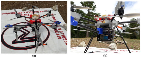
Figure 1.
(a) The hexa-coaxial copter; (b) the LasUAV Light Detection and Ranging (LiDAR) system mounted in the unmanned aerial vehicle (UAV).
2.2. Study Area
The study area was located on Monte Morello (934 m ASL) at N43°52’55.92” and E11°13’53.04” in the NW side of Florence (Italy). In the historic past, this mountain area was affected by an intensive browsing and grazing that altered the forest vegetation [49] and triggered hydrogeological instability. During the last century, the area was therefore subject to reforestation concluded in the early 1980s. Conifer species, in particular European black pine (Pinus nigra J. F. Arnold), Brutia pine (Pinus brutia Ten.), Mediterranean cypress (Cupressus sempervirens L.) and Atlas cedar (Cedrus atlantica (Endl.) Carrière), were chosen for their capability to colonize bare-earth with occasional broadleaves such as Turkey oak (Quercus cerris L.) and leaving already existing native trees such as downy oak (Quercus pubescens Willd.). Nowadays, the stands consist of two-layered mixed even-aged high forest. The upper layer was composed of dominant trees where coniferous species and oaks were prevailing; the bottom layer consisted of overtopped trees where the presence of manna ash (Fraxinus ornus L.), field maple (Acer campestre L.) and hawthorn (Crataegus monogyna Jacq.) was significant in terms of number of trees, but less significant in terms of biomass. Table 1 summarizes the characteristics of the study area.

Table 1.
Characteristics of Monte Morello study area.
2.3. Reference Data
Since 2016, the Monte Morello study area has been sampled within the LIFE14 CCM/IT/000905 FoResMit (Recovery of degraded coniferous Forests for environmental sustainability Restoration and climate change Mitigation) Project: 18 circular plots of 13 m of radius (530.93 m2) were sampled (Figure 2). Three plots, positioned in the northeast side of the study area, were selected for this study.
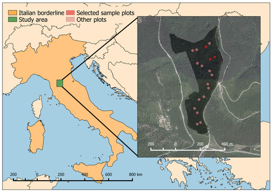
Figure 2.
The location of the study area within the Italian national borders and the distribution of 18 plots with the 3 plots under investigation in this study (dark red) within the study area.
Field surveys were carried out from June to September 2016, in leaf-on period. For each tree with DBH bigger or equal to 3.5 cm, the species, the health state (unharmed, broken or dead) and the DBH were recorded. The polar coordinates of each tree were collected using a TruPulse Laser Rangefinder 200/B (Laser Technology, Inc., Centennial, USA) and then converted into Cartesian coordinate with origin in the plot center. For a subsample of 10 trees per plot, the height was also measured with the rangefinder-hypsometer Haglöf Vertex IV (Haglöf Sweden AB, Sverige, Sweden). These trees were selected to distribute height measures along the DBH range for each plot and to measure only trees with very visible tops. To estimate the height of the trees for which only DBH was measured in the field, a bivariate model was fitted with the function aov() of R [50] using log(DBH) as a continuous predictor, tree species as a categorical predictor and measured tree heights as the dependent variable
The model then estimates tree height (H) as:
where a and b are the model intercept and slope, and DBH is the stem diameter at 1.3 m height. [Species] is the categorical predictor on which the model builds the contrast matrix and is composed by the following 8 categories: (i) Acer campestre, (ii) Cupressus sempervirens, (iii) Fraxinus ornus, (iv) Pinus nigra, (v) Pinus brutia, (vi) Quercus cerris, (vii) other conifers and (viii) other broadleaves. A leave-one-out cross validation algorithm was used to estimate the model accuracy. Model accuracy resulted in a root-mean-square error (RMSE) of 1.77 m, a mean absolute error (MAE) of 1.36 m, while the errors percentiles resulted: 5% = −2.73 m, 12.5% = −1.80 m, 50% = 0.05 m, 87.5% = 1.92 m, 95% = 2.66 m.
Volume for all live, unbroken trees was computed using the equations developed by [51] for the second Italian national forest inventory which allows the prediction of the total above ground biomass using DBH and total tree height as independent variables for twenty-five of the most important forest species growing in Italy.
A univariate analysis of variance (ANOVA), followed by a multiple comparison of tree height means, was used to identify statistically significant differences between the biometric parameters of each species, giving insight on species-specific effects on the algorithms’ output. Both the ANOVA and the multiple comparison test were part of the Statistics and Machine Learning Toolbox of MATLAB R2017a (functions anova1 and multcompare, MathWorks, Inc., Natick, MA, USA).
The dendrometric features of each plot are reported in Table 2.
Table 2.
Description of dendrometric features of the 3 plots investigated. CV is the coefficient of variation for the given variable and DBH is the diameter at breast height.
In plot 6.1, 24.2% of total trees were present in the canopy layer and the remaining 75.8% in the understory layer. In plot 6.2, 43.8% of total trees were present in the canopy layer and the remaining 56.3% in the understory layer. In plot 7.2, 64.8% of total trees were present in the canopy layer and the remaining 35.2% in the understory layer.
2.4. LiDAR Data Acquisition and Point Cloud Pre-processing
LiDAR data acquisition was carried out on 28 July 2017. The flight altitude was on average 50 m above ground level, the flying speed was 2.5 m/s and the flight sampling time was 10 min. A total of 8 flight lines, which resulted in a flight line spacing of about 20 m, were necessary to cover the 155 m × 102 m area where plots 6.1, 6.2 and 7.2 were located. Based on a ±30° scanning angle, the average point density was about 193 points/m2. A summary of the characteristics of the UAV flight and LiDAR data collected is reported in Table 3.
Table 3.
Summary of the characteristics of the unmanned aerial vehicle (UAV) flight and light detection and ranging (LiDAR) data collected during the survey of 28 July 2017.
The whole point cloud gathered by the LiDAR is shown in Figure 3a, while a slice of the cloud highlighting the two-layered structure of the canopy is shown in Figure 3b.
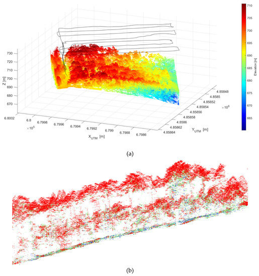
Figure 3.
LiDAR point cloud with UAV trajectory in black line, universal transverse Mercator (UTM) coordinates in the X and Y axis (in m) and ellipsoidal height (Z, in m) (a) and slice of the point cloud, with points colored by return number (red, first return; green, second return; blue, third return), evidencing the two layered structure of the forest (b).
After full point cloud production, three subsets were extracted as cylinders with a radius of 16 m centered at each plot. The choice of the radius larger than the field plot size (13 m) was made to avoid “edge effects” that would have produced the loss of data points belonging to trees with stem inside the plot but crown partially outside. On the other hand, trees with the stem outside and crown partially inside plot boundaries were excluded after their segmentation based on their location outside the plot border.
2.5. Individual Tree Crown Delineation Approach and Trees Matching
This approach was translated by [52] in the itcLiDAR() function contained in the itcSegment package which was used in this study. In the itcLiDAR() function, in addition to the x,y,z coordinates of each LiDAR return and the coordinate reference system, the input parameters defined in Table 4 were provided.
Table 4.
Input parameters of itcLiDAR() function and their definition. In the definition CHM stands for canopy height model.
From the itcLiDAR() function, x,y coordinates, height and crown area of each tree were obtained. The dbh() function of itcSegment was then used to predict the DBH of each delineated tree crown and the agb() function, based on the equations developed by [48], was used to predict AGB of each delineated tree crown. To ensure that the itcLiDAR() function performed optimally for the dense mixed forest under investigation, a tuning of input parameters was made (Table 4). On each plot, a single parameter was varied in a wide interval while maintaining the others (i.e., resolution and cw) fixed according to the ecological meaning of the parameter and the level of knowledge of forest stands characteristics (Table 5). This procedure resulted in a set of 1350 parameter combinations.
Table 5.
Range of parameter values set to tune the itcLiDAR() function. Parameters with a “-“ in the Step column were kept fixed, while Min and Max columns indicate the range of variation for the given parameter.
For each combination, the delineated trees were matched to the field surveyed trees using the [53] method: if only one field-measured tree was included inside a delineated crown, then that tree was associated with the corresponding segmented tree; otherwise if more than one field-measured tree was included in a segmented crown, the field-measured tree with the height closer to the segmented tree height was chosen.
For each plot and for each combination of itcLiDAR() function parameters the ITC delineation accuracy (accuracy index, AI) was computed as:
where OE is the omission error, i.e., existing trees not detected; CE is the commission error, i.e., delineated crowns that do not exist in reality. Detection rate (DET) was computed as the ratio between the number of matched trees and the number of trees measured in field. The best set of itcLiDAR() function parameters was the one that maximized AI.
AI = 100 − (OE + CE)
At tree level, for each delineated tree crown, DBH and height measured in the field and volume computed from the second Italian national forest inventory equations, were compared to the corresponding variables resulting from the UAV point cloud processing with the itcSegment() package. A comparison between the DBH frequency distribution from both datasets was also performed.
At plot level, for the entire set of matched trees a comparison between average tree density, DBH, height and AGB was made. The AGB estimate uncertainty was calculated as the percentage difference between AGB estimated from the UAV-LS data and from second Italian national forest inventory equations.
For comparison, the approach of individual tree crowns delineation developed by [47] was accomplished. The algorithm, developed for small footprint discrete return ALS point cloud, segments individual trees in a sequence by taking advantage of the relative spacing between trees. Starting from a treetop, the algorithm identifies and “grows” a target tree by including nearby points and exclude points of other trees based on their relative spacing. To overcome the difficulty of classifying points at lower level due to the diminished spacing between trees, points were classified sequentially, from the highest to the lowest. Points with spacing larger than a specified threshold were excluded from the target tree; points with spacing smaller than the threshold were classified based on a minimum spacing rule [47]. This segmentation method is contained in the li2012 algorithm in the lastrees() function of lidR package [54]. A parameter tuning procedure similar to the one used for tuning the itcLiDAR() function was applied, varying the value of li2012 algorithm parameters in the ranges reported in Table 6.
Table 6.
Input parameters of li2012 algorithm in lastrees() function, their definition and their range of values.
3. Results
3.1. Calibration of itcLiDAR() Function Parameters
For each of the three plots, the optimal combination of itcLiDAR() function parameters obtained with the iterative tuning procedure is reported in Table 7.
Table 7.
itcLiDAR() function parameter values allowing the best level of accuracy.
The value of maximum size in pixels of the moving window used to detect the local maxima of the CHM (MaxSearchFilSize) was the same in the three plots. The minimum size was equal in plots 6.1 and 6.2, while changed in plot 7.2 that was characterized by a lower tree density and a higher mean DBH. This means that in stands with mature trees, the value of the minimum size of the moving window was close to the maximum, due to a lower crown size variability. Similarly, both the maximum crown diameter of a detected tree (maxDIST) and the first threshold of the minimum vertical distance between the height of each neighbor pixel extracted from the CHM and the height of the local maximum (TRESHSeed) were the same in plot 6.1 and 6.2 and different in plot 7.2. The second threshold of the minimum vertical distance between the height of each neighbor pixel extracted from the CHM and the height of the local maximum (TRESHCrown) and the minimum value of the crown diameter of a detected tree (minDIST) had different values in each plot after the tuning process (Table 7).
3.2. ITC Detection and Dendrometric Variables Estimation with the itcLiDAR() Function
The known position of individual trees over imposed to the crowns delineated by the itcLiDAR() function is reported in Figure 4.
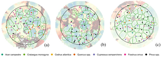
Figure 4.
Comparison between the position of trees field surveyed (red points) and the crowns delineated by itcLiDAR() function (green polygons) in plots 6.1 (a), 6.2 (b) and 7.2 (c).
Detection rate ranged between 40% to 57%, omission error between 42% and 59% and commission error between 41% and 53% (Table 8). The highest detection rate and overall accuracy was obtained in plot 7.2, characterized by a lower tree density and with 65% of trees (composed by European black pine, Brutia pine and Mediterranean cypress) in the upper layer and 35% in the understory. This indicates that plot 7.2 was easier to segment due to the shape of conifer crowns that allowed the clear identification of the apex. Quite high levels of under segmentation were obtained in plot 6.1 and 6.2 where the overlap between close trees was relevant, being the plot density very high.
Table 8.
ITC delineation accuracy for three plots (DET = detection rate, crown correctly detected, OE = omission error, failure to detected a crown that exists, CE = commission error, delineation of a crown that do not exists in reality, AI = accuracy index, 100 - (OE + CE).
In plot 6.1 and 6.2, DBH of small trees was estimated successfully, while DBH of medium and large trees was underestimated by the segmentation process. In these two plots, tree density was high because of a large presence of small trees in the understory (75% and 56% in plot 6.1 and 6.2 respectively), but at the same time there were canopy gaps that facilitated the identification of individual crowns (Figure 4). Instead, in plot 7.2, DBH of small trees was over-estimated while DBH of medium and large trees was under-estimated (Figure 5).
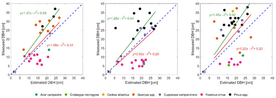
Figure 5.
Estimation of the diameter at breast height (DBH) for the field-measured trees (measured DBH, y-axis) by the segmentation process (estimated DBH, x-axis) in plots 6.1 (a), 6.2 (b) and 7.2 (c). Red lines and associated statistics show linear fits (with the intercept forced to zero) considering the whole dataset, while green lines and statistics show the linear fit after removing the cluster of shorter species (field maple, hawthorn and manna ash). The blue dashed line indicates the 1:1 reference line in all the three plots.
Individual tree crown delineation was successful for trees with DBH larger than 10 cm (detection rate of 78.3%, 50.0% and 67.6% for plot 6.1, 6.2 and 7.2 respectively), while failed to detect trees with DBH smaller than 10 cm (detection rate of 19.5%, 33.5% and 36.8% for plot 6.1, 6.2 and 7.2 respectively). The algorithm over-segmented trees with DBH between 16 and 24 cm, while under-segmented trees with DBH between 28 and 36 cm (Figure 6).
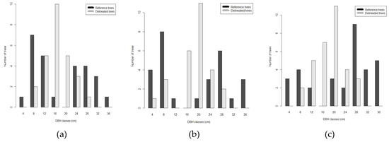
Figure 6.
Comparison between the distribution frequency of DBH field surveyed (black) and the distribution frequency from dbh() function (gray) in plots 6.1 (a), 6.2 (b) and 7.2 (c).
In all the three plots, tree heights around 10 m and in the range between 15 to 20 m were quite well estimated, while in the range between 10 to 15 m they were overestimated by about 50%. In terms of tree species, height overestimation especially affects species that were significantly shorter (field maple, hawthorn, manna ash, p < 0.05 for the ANOVA test) and that clearly cluster separately from the other species (Figure 7). Linear fitting between measured and derived heights (red lines and statistics, Figure 7a–c) strongly improves when removing such cluster of shorter species from the dataset (green lines and statistics, Figure 7a–c).
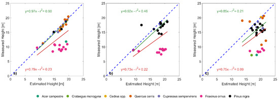
Figure 7.
Measured and estimated tree height for the field-measured trees in plots 6.1 (a), 6.2 (b) and 7.2 (c). Colors of the dots identify the tree species. Red lines and associated statistics show linear fits (with the intercept forced to zero) considering the whole dataset, while green lines and statistics show the linear fit after removing the cluster of shorter species (field maple, hawthorn and manna ash). The blue dashed line indicates the 1:1 reference.
The correlation between tree species and height overestimation also affects RMSE between measured and estimated height when pooling the data by species rather than by plot (Figure 8). The RMSE shows a strong inverse correlation with the average measured species height. Field maple (with an average height of 9.37±2.31 m) has the highest RMSE (9.75 m), while the Atlas cedar (single exemplar with a measured height of 20.2 m) has the lowest RMSE (0.07 m).
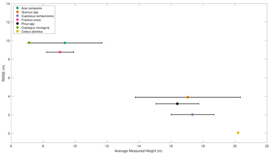
Figure 8.
Correlation between the average measured height by species and root-mean-square error (RMSE) with estimated height. Species are indicated by the color of the dot, while the error-bars show ± the standard deviation of height for the given species.
The total above ground biomass estimated for each tree was compared with field estimates in Figure 9. An overall bias was obtained, with the biomass of small trees resulting overestimated and that of large trees underestimated.
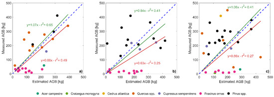
Figure 9.
Estimation of the above ground biomass (estimated AGB, x-axis) for the field-measured trees (measured AGB, y-axis) in plots 6.1 (a), 6.2 (b) and 7.2 (c). Red lines and associated statistics show linear fits (with the intercept forced to zero) considering the whole dataset, while green lines and statistics show the linear fit after removing the cluster of shorter species (field maple, hawthorn and manna ash). The blue dashed line indicates the 1:1 reference.
Table 9 reports a comparison between average value of tree density, DBH, height and AGB at plot level. Considering the average values of above ground biomass measured in the field and estimated by the individual tree delineation process, the biomass estimates uncertainty resulted about 13%, 41% and −9% for plot 6.1, 6.2 and 7.2 respectively. The algorithm, instead, tends to overestimate both mean height and mean DBH (with the exception of DBH in plot 7.2).
Table 9.
Tree number, mean DBH, mean height, total above ground biomass (AGB) estimation field surveyed (= FS) and derived from itcLiDAR() function (= UAV).
3.3. Calibration of Function Parameters, ITC Detection and Dendrometric Variables Estimation with the li2012 Algorithm in Lastrees() Function
The optimal set of parameters of the li2012 algorithm after the iterative tuning procedure for each plot is reported in Table 10.
Table 10.
Parameters of li2012 algorithm in the lastrees() function allowing the best level of accuracy.
Figure 10 reports the segmented crowns of trees with respect to the position of tree stems surveyed in field, showing a clear tendency of the algorithm to aggregate the crowns of more than one tree and consequently delineate bigger crowns than in reality.
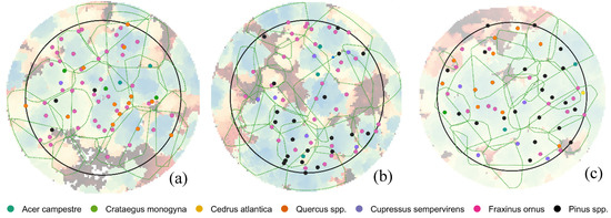
Figure 10.
Comparison between the position of trees field surveyed (red points) and the crowns delineated by itcLiDAR() function (green polygons) in plots 6.1 (a), 6.2 (b) and 7.2 (c).
Values of detection rate are quite far from those obtained with the application of itcLiDAR, varying between 25% and 27% (Table 11). In case of plot 6.1 a value of commission error equal to 0% was obtained because no segmented trees were not matched: indeed, as the obtained crowns had a large diameter there were always one or more field measured tree inside the delineated crown.
Table 11.
ITC delineation accuracy for three plots using lastrees() function.
As the level of accuracy reached by li2012 algorithm in lastrees() was very low, no details in the performance DBH, height and AGB are provided and the following discussion is therefore focused on the best-performing algorithm.
4. Discussion
Delineation accuracy of ITC segmentation obtained in this study was in line with other studies based on ALS. Ref. [55] evaluated the quality, accuracy and feasibility of nine automatic tree extraction methods based on ALS data acquired in boreal forest stands with point densities of 2, 4 and 8 points/m2. The capabilities of detecting trees resulted between 25% and 102%, while the point density had a minor impact on the segmentation rate. The commission error varied between 0% and 26.5%, while the omission error varied between 35% and 68%. As expected, the taller trees were detected with a better accuracy; the RMSE of height estimation for the delineated trees ranged from 60 to 80 cm for the best methods. Ref. [45] benchmarked eight ALS tree detection methods, including the method that was used here [53], across different regions, forest types and structures in the Alps. Considering all the methods, the omission error ranged between 51% and 63%, being higher for multi-layered mixed and coniferous forests and lower for single-layered coniferous forest (37%). The method of [53] that was used here produced an overall omission error of 61%, while the omission error in single layered mixed forests was 25%, in single layered coniferous forests was 40%, in multi layered mixed forests was 75% and in multi layered coniferous forest was 65%. Ref. [56] benchmarked five ALS-based individual tree detection methods with a point cloud density of 2, 4 and 8 points/m2 acquired in five boreal forests with diverse stand conditions and different developmental stages (i.e., from deciduous-dominated to mixed, to coniferous-dominated and from old to mature to very young stands) considering four crown classes, i.e., dominant, codominant, intermediate and suppressed trees. Their study revealed that omission error varied between 25% and 63% and that all methods tended to overestimate the number of dominant trees and underestimate the number of subordinate trees. Delineation of dominated trees was challenging for all methods.
Similar to [45,55,56], one finding of our study was that the omission error varies between 40% and 57% and that the largest fraction of not detected trees was in the understory, which suggests they were dominated trees. This outcome, that needs to be confirmed by further studies considering larger datasets, confirms what [55] highlighted concerning the effect of point density on the ITC delineation accuracy and retract the outcomes of [56]: high levels of laser point density do not increase the delineation accuracy. In fact, also using LiDAR data with very high density as in this study (i.e., 193 points/m2) the accuracy of tree segmentation was similar to that obtained in the studies that benchmarked individual tree detection methods using ALS data with point density ranging from 2 to 8 points/m2.
The most important experiences in using UAV-borne LiDAR data for ITC delineation are from [15,36,38,57,58,59].
Ref. [15] used high-resolution LiDAR data captured from a small multirotor UAV to extract individual trees in 6 circular plots in a four-year-old Tasmanian blue gum regular plantation (density ranging from 680 to 1560 trees/ha) located in Southern Tasmania (Australia) using an adaptation of the method outlined by [47]. By means of this approach, 91% of field-measured trees were correctly matched to the UAV segmented trees across all plots. In their successive study, Ref. [57], using the same data set, tested five tree detection routines to assess the tree delineation accuracy. The percentage of field-measured trees correctly matched with UAV-LS delineated trees resulted between 92% and 97%. The highest rate of omission occurred in small trees, while commission errors for most algorithms was caused by over-segmentation of large trees. The study also highlighted that improvement in omission rate occurs using higher point densities (~50 points/m2).
Ref. [36] delineated trees from UAV-borne laser scanner data acquired over a 64 m × 64 m study area located in Evo, Southern Finland, with a density of about 490 trees/ha. A two steps approach for individual tree detection was used, based on the application of a local maximum filtering algorithm on the CHM and on the application of a watershed algorithm to successively delineate the tree crowns. The average detection rate resulted 84.2%, being 100% for isolated and dominant trees, but the relatively low value of tree density of the study area, facilitating the detection process, should be considered. When utilizing direct measurement in the point cloud, Ref. [36] obtained a relative RMSE equal to 6.47% in height estimation and 27.46% in DBH estimation.
Ref. [38] delineated individual tree crows from UAV-LS data acquired in an ecotone area in Northern Arizona (USA) which includes a shrubland-grassland meadow adjacent to a ponderosa pine forest with a density of 220 trees/ha. They obtained a determination coefficient between the number of trees delineated from the LiDAR data and field-based tree density equal to 0.77 and a determination coefficient for tree height within dense canopy cover equal to 0.79, where only the tallest tree canopy heights were successfully estimated and the shorter trees under the tall canopies were missed by the laser scanner.
Ref. [58] applied a methodology to UAV-LS data based on fitting and modeling the 3D-shape of trees in a hazel grove using RANSAC [59] obtaining a detection rate equal to 86%.
Ref. [60] assessed the performance of four algorithms (three based on CHM and one on point cloud) for individual tree detection using UAV-LS data in pure ginkgo planted forest in China with density ranging from 400 to 700 trees per hectare, DBH ranging from 16 cm to 20 cm and Lorey’s height from 12 m to 11 m. The individual tree detection algorithm based on point cloud was the best performing in plot with low density but was the worst as the tree density increased.
Unlike our study, that was conducted in multi-layer forest stands with a density higher than 1000 trees/ha and with a high level of crown cover, the results of the studies reported above were obtained in isolated trees, in stands composed by only dominated trees, in plantation where trees were planted with a regular pattern, and overall, in stands with a tree density approximately half of that of our analysis. And as a matter of fact, the levels of accuracy obtained in our study were slightly lower. The optimal setting of itcLiDAR() function has determined a detection rate ranging between 40% and 57% in the three plots, while the main source of omission error was the failure to separate two or three medium trees that have similar heights and were located close to each other. The tuning of the ITC algorithm parameters resulted quite important in reaching the highest determination rates that ranged from 23.4% to 40.6% in plot 6.1, 21.2% and 40.9% in plot 6.2 and 32.1% and 57.1% in plot 7.2 across the parameter optimization space. This was an important outcome: knowing the possible range of variability of each parameter was the starting point for the individual tree segmentation process to reach the optimal determination rates. Hence, the application of a parameter tuning procedure is suggested to optimize the segmentation process for a specific set of forest characteristics. Our findings agree with [44], which reports that a certain degree of calibration is necessary to obtain the best results in tree detection and delineation, where size and shape of the 3D kernel play a crucial role. Another reason that explains the lower values of detection rate obtained here with respect to other studies is the approach used to match the delineated trees with the field surveyed trees. The approach of [53] considers the inclusion of a field-measured tree inside the delineated crown and difference of height between the field measured tree and the delineated tree. Other methods consider also the planar distance between delineated and reference trees (i.e., [61]) or the maximum values of height differences (i.e., [62]). Depending on the method used for tree matching, the results can be quite different. Vertical forest stratification in combination with the matching process were probably the factors that have determined the overestimation of canopy height. Intermediate trees, that occupied a position underneath the dominant and co-dominants trees, were erroneously coupled with the higher trees. Indeed, in some cases crowns of dominant trees, due to the specific shape of species present in the stands, were segmented as two distinct trees, so in this way a delineated tree was coupled with the dominant tree and the other one with the codominant or intermediate tree, leading to an over estimation of tree height and consequently of tree biomass.
The effect of stratification on the estimation of tree heights was clearly visible when removing shorter trees from the analysis. The coefficient of determination for estimated versus measured tree height, in fact, greatly increased when significantly shorter trees were removed, reaching even higher values than [38] in plot 6.1 (0.90 vs. 0.79). In fact, when considering individually the single species, the effect of stratification was relevant: taller species that stand out clearly from the dense mixed canopy have lower RMSEs between measured and estimated heights, while shorter species were less easily distinguished and have associated higher errors. We should also consider the error that occur during the ground-based tree height measurements which was related to the tree top shape, determined by the apical dominance: the higher the apical dominance, the greater the ability to detect the tree top in field survey. This implies that in species with a strong apical dominance (e.g., Atlantic cedar and Mediterranean cypress) the uncertainty in tree height field measurement was lower than in species with moderate or low apical dominance (e.g., European black pine and Turkey oak). This aspect reflects in the RMSE that was lower in species with greater apical dominance (Figure 8).
This study was based on a sample size of 186 trees, which could prevent the upscaling of the results obtained here to larger areas. However, comparable sample sizes were used in several studies focusing on small areas without loss of generality [58]. Ref. [43] employed UAV-LS data to build 200 tree models by a quantitative structure approach and compared them with terrestrial laser scanning obtaining reliable volume estimations for trunks and branches ≥ 30 cm. Similarly, Ref. [44] used multiple segmentation algorithms over about 120 trees, while [58] performed 3D volume reconstruction with UAV-LS on 181 hazel trees. Overall, these studies increase the confidence in the validity of the approach proposed here, that definitely calls for further and deeper analysis based on forthcoming larger datasets.
5. Conclusions
This study explored the application of two different algorithms, i.e., itcLiDAR() and li2012, for individual tree crown segmentation in a two-layered dense mixed forest. The parameters of both algorithms were tuned for this experimental site through an optimization procedure. The raster-based local maxima region growing algorithm itcLiDAR() performed better than the point cloud-based li2012 and the performance of its estimates resulted comparable to those obtained in ITC segmentation based on ALS data. The parameters calibration for individual tree crown detection was necessary and allowed to increase the performance of the segmentation process. The accuracy obtained with the method based on CHM maxima was reasonable for forest inventory, but still not satisfactory. In fact, such method proved to be very efficient for forests composed by conifers with a well-defined apex (i.e., European spruce, fir, European larch) and with uniform height implying they were not multilayered. In presence of broadleaved forests, forests composed by trees having round, broad, spreading and irregular crowns—or in the case of mixed multilayered forests—the segmentation procedure becomes challenging. The exploration of algorithms—other than those based on generating a CHM and searching for local maxima in the top of the canopy indicating the position of the tree—is needed. These should allow achieving higher detection rates and accuracy on dendrometric variables estimated across a wide range of species and in multilayered forests where most of trees were hidden under or between taller and larger trees. Given the complex and heterogeneous structure of many forests it is important that future research is conducted in this direction, assuming that the main advantage of individual tree detection stays in the capacity to provide true stem distribution series, enabling accurate estimates of timber assortments.
Author Contributions
Conceptualization, C.T., U.C. and B.G.; Data Curation, C.T. and B.G.; formal analysis, C.T. and U.C.; funding acquisition, C.T., U.C., F.M. and A.Z.; investigation, C.T., F.C., U.C. and B.G.; methodology, C.T., F.C., U.C. and B.G.; project administration, C.T., U.C., F.M., A.Z. and B.G.; resources, C.T., U.C., F.M. and A.Z.; software, C.T., F.C. and B.G.; supervision, F.M. and B.G.; validation, C.T. and B.G.; Visualization, C.T. and U.C.; writing-Original Draft, C.T.; writing-Review & Editing, C.T., F.C., U.C. and B.G. All authors have read and agreed to the published version of the manuscript.
Funding
This research was funded in part by the CARITRO Foundation under project UAV4PRECIFOR (2014.0408, 2143/14) and in part by the Tuscany Region under project SPIRIT (plan POR FESR 2014–2020 for research and development). The field survey was realized also with the contribution of FoResMit project (LIFE14 CCM/IT/000905).
Acknowledgments
The authors wish to thank Andrea Berton for skillfully piloting the UAV in this experiment and the companies that contributed to the LasUAV system in the frame of the SPIRIT project: D.R.E.Am Italia (Pratovecchio, AR, Italy), Wolf s.r.l. (Firenze, FI, Italy) and G.S.T. Italia s.p.a. (Signa, FI, Italy).
Conflicts of Interest
The authors declare no conflict of interest.
References
- Vauhkonen, J.; Maltamo, M.; McRoberts, R.E.; Næsset, E. Introduction to Forestry Applications of Airborne Laser Scanning. In Forestry Applications of Airborne Laser Scanning. Managing Forest Ecosystems; Maltamo, M., Næsset, E., Vauhkonen, J., Eds.; Springer: Dordrecht, The Netherlands, 2014; Volume 27. [Google Scholar]
- Næsset, E. Determination of mean tree height of forest stands using airborne laser scanner data. J. Photogramm. Remote Sens. 1997, 52, 49–56. [Google Scholar] [CrossRef]
- Persson, Å.; Holmgren, J.; Söderman, U. Detecting and measuring individual trees using an airborne laser scanner. Photogramm. Eng. Remote Sens. 2002, 68, 925–932. [Google Scholar]
- Solberg, S.; Naesset, E.; Bollandsas, O.M. Single tree segmentation using airborne laser scanner data in a structurally heterogeneous spruce forest. Photogramm. Eng. Remote Sens. 2006, 72, 1369–1378. [Google Scholar] [CrossRef]
- Sačkov, I.; Scheer, L.; Bucha, T. Predicting forest stand variables from airborne LiDAR data using a tree detection method in Central European forests. Cent. Eur. For. J. 2012, 65, 191–197. [Google Scholar] [CrossRef]
- Lovell, J.L.; Jupp, D.L.B.; Culvenor, D.S.; Coops, N.C. Using airborne and ground-based ranging lidar to measure canopy structure in Australian forests. Canadian J. Remote Sens. 2003, 29, 607–622. [Google Scholar] [CrossRef]
- Naesset, E. Estimating timber volume of forest stands using airborne laser scanner data. Remote Sens. Environ. 1997, 61, 246–253. [Google Scholar] [CrossRef]
- Hollaus, M.; Wagner, W.; Maier, B.; Schadauer, K. Airborne Laser Scanning of Forest Stem Volume in Mountainous Environments. Sensors 2007, 7, 8–19. [Google Scholar] [CrossRef]
- Maltamo, M.; Eerikäinen, K.; Pitkänen, J.; Hyyppä, J.; Vehmas, M. Estimation of timber volume and stem density based on scanning laser altimetry and expected tree size distribution function. Remote Sens. Environ. 2004, 90, 319–330. [Google Scholar] [CrossRef]
- Gobakken, T.; Næsset, E. Estimation of diameter and basal area distributions in coniferous forest by means of airborne laser scanner data. Scand. J. Forest Res. 2004, 19, 529–5242. [Google Scholar] [CrossRef]
- Holmgren, J. Prediction of tree height, basal area and stem volume in forest stands using airborne laser scanning. Scand. J. Forest Res. 2004, 19, 543–553. [Google Scholar] [CrossRef]
- Næsset, E. Accuracy of forest inventory using airborne laser scanning: Evaluating the first nordic full-scale operational project. Scand. J. For. Res. 2004, 19, 554–557. [Google Scholar] [CrossRef]
- Næsset, E. Airborne laser scanning as a method in operational forest inventory: Status of accuracy assessments accomplished in Scandinavia. Scand. J. For. Res. 2007, 22, 433–442. [Google Scholar] [CrossRef]
- Torresan, C.; Berton, A.; Carotenuto, F.; Chiavetta, U.; Miglietta, F.; Zaldei, A.; Gioli, B. Development and Performance Assessment of a Low-Cost UAV Laser Scanner System (LasUAV). Remote Sens. 2018, 10, 1094. [Google Scholar] [CrossRef]
- Wallace, L.; Lucieer, A.; Watson, C.S. Evaluating tree detection and segmentation routines on very high resolution UAV LiDAR data. Trans. Geosci. Remote Sens. 2014, 52, 7619–7628. [Google Scholar] [CrossRef]
- Amon, P.; Rieger, P.; Riegl, U.; Pfennigbauer, M. Introducing a New Class of Survey–Grade Laser Scanning by use Unmanned Aerial Systems (UAS). In Proceedings of the FIG Congress 2014, Engaging the Challenges–Enhancing the Relevance, Kuala Lumpur, Malaysia, 16–21 June 2014. [Google Scholar]
- Amon, P.; Riegl, U.; Rieger, P.; Pfennigbauer, M. UAV-based laser scanning to meet special challenges in lidar surveying. In Proceedings of the Geomatics Indaba 2015–Stream 2, Ekurhuleni, South Africa, 11–13 August 2015. [Google Scholar]
- Yao, H.; Qin, R.; Chen, X. Unmanned Aerial Vehicle for Remote Sensing Applications—A Review. Remote Sens. 2019, 11, 1443. [Google Scholar] [CrossRef]
- Ota, T.; Ogawa, M.; Shimizu, K.; Kajisa, T.; Mizoue, N.; Yoshida, S.; Takao, G.; Hirata, Y.; Furuya, Y.; Sano, T.; et al. Aboveground Biomass Estimation Using Structure from Motion Approach with Aerial Photographs in a Seasonal Tropical Forest. Forests 2015, 6, 3882–3898. [Google Scholar] [CrossRef]
- Wallace, L.; Lucieer, A.; Malenovský, Z.; Turner, D.; Vopěnka, P. Assessment of Forest Structure Using Two UAV Techniques: A Comparison of Airborne Laser Scanning and Structure from Motion (SfM) Point Clouds. Forests 2016, 7, 62. [Google Scholar] [CrossRef]
- Baltsavias, E.P. A comparison between photogrammetry and laser scanning. ISPRS J. Photogramm. Remote Sens. 1999, 54, 83–94. [Google Scholar] [CrossRef]
- White, J.C.; Wulder, M.A.; Vastaranta, M.; Coops, N.C.; Pitt, D.; Woods, M. The Utility of Image-Based Point Clouds for Forest Inventory: A Comparison with Airborne Laser Scanning. Forests 2013, 4, 518–536. [Google Scholar] [CrossRef]
- Leberl, F.; Irschara, T.; Pock, T.; Meixner, P.; Gruber, M.; Scholz, S.; Wiechert, A. Point clouds: Lidar versus 3D vision. Photogramm. Eng. Remote Sens. 2010, 76, 1123–1134. [Google Scholar] [CrossRef]
- Goodbody, T.R.H.; Coops, N.C.; White, J.C. Digital Aerial Photogrammetry for Updating Area-Based Forest Inventories: A Review of Opportunities, Challenges, and Future Directions. Curr. For. Rep. 2019, 5, 55–75. [Google Scholar] [CrossRef]
- White, J.C.; Stepper, C.; Tompalski, P.; Coops, N.C.; Wulder, M.A. Comparing ALS and Image-Based Point Cloud Metrics and Modelled Forest Inventory Attributes in a Complex Coastal Forest Environment. Forests 2015, 6, 3704–3732. [Google Scholar] [CrossRef]
- White, J.C.; Tompalski, P.; Coops, N.C.; Wulder, M.A. Comparison of airborne laser scanning and digital stereo imagery for characterizing forest canopy gaps in coastal temperate rainforests. Remote Sens. Environ. 2018, 208, 1–14. [Google Scholar] [CrossRef]
- Jakubowski, M.K.; Li, W.; Guo, Q.; Kelly, M. Delineating Individual Trees from Lidar Data: A Comparison of Vector- and Raster-based Segmentation Approaches. Remote Sens. 2013, 5, 4163–4186. [Google Scholar] [CrossRef]
- Tomaštík, J.; Mokroš, M.; Saloň, Š.; Chudý, F.; Tunák, D. Accuracy of Photogrammetric UAV-Based Point Clouds under Conditions of Partially-Open Forest Canopy. Forests 2017, 8, 151. [Google Scholar] [CrossRef]
- Goodbody, T.R.; Coops, N.C.; Hermosilla, T.; Tompalski, P.; Pelletier, G. Vegetation Phenology Driving Error Variation in Digital Aerial Photogrammetrically Derived Terrain Models. Remote Sens. 2018, 10, 1554. [Google Scholar] [CrossRef]
- Jozkow, G.; Toth, C.; Grejner-Brzezinskaa, D. UAS Topographic mapping with velodyne LiDAR sensor. In ISPRS Annals of the Photogrammetry, Remote Sensing and Spatial Information Sciences; Volume III-1, 2016 XXIII; ISPRS Congress: Prague, Czech Republic, 2016. [Google Scholar] [CrossRef]
- Jozkow, G.; Wieczorek, P.; Karpina, M.; Walicka, A.; Borkows, A. Performance evaluation of a sUAS equipped with Velodyne HDL-32E LiDAR sensor. Int. Arch. Photogramm. Remote Sens. Spatial Inf. Sci. 2017, XLII-2/W6, 171–177. [Google Scholar] [CrossRef]
- Torres, F.M.; Tommaselli, A.M.G. A lightweight uav-based laser scanning system for forest application. Bull. Geod. Sci. 2018, 24, 318–334. [Google Scholar] [CrossRef]
- Chisholm, R.A.; Cui, J.; Lum, S.K.Y.; Chen, B.M. UAV LiDAR for below-canopy forest surveys. J. Unmanned Veh. Syst. 2013, 1, 61–68. [Google Scholar] [CrossRef]
- Morsdorf, F.; Eck, C.; Zgraggen, C.; Imbach, B.; Schneider, F.D.; Kükenbrink, D. UAV-based LiDAR acquisition for the derivation of high-resolution forest and ground information. Leading Edge 2017, 36, 566–570. [Google Scholar] [CrossRef]
- Wieser, M.; Mandlburger, G.; Hollaus, M.; Otepka, J.; Glira, P.; Pfeifer, N. A Case Study of UAS Borne Laser Scanning for Measurement of Tree Stem Diameter. Remote Sens. 2017, 9, 1154. [Google Scholar] [CrossRef]
- Jaakkola, A.; Hyyppä, J.; Yu, X.; Kukko, A.; Kaartinen, H.; Liang, X.; Hyyppä, H.; Wang, Y. Autonomous collection of forest field reference—The outlook and a first step with UAV laser scanning. Remote Sens. 2017, 9, 785. [Google Scholar] [CrossRef]
- Guo, Q.; Su, Y.; Hu, T.; Zhao, X.; Wu, F.; Li, Y.; Liu, J.; Chen, L.; Xu, G.; Lin, G.; et al. An integrated UAV-borne lidar system for 3D habitat mapping in three forest ecosystems across China. Int. J. Remote Sens. 2017, 38, 2954–2972. [Google Scholar] [CrossRef]
- Sankey, T.; Donager, J.; McVay, J.; Sankey, J.B. UAV lidar and hyperspectral fusion for forest monitoring in the southwestern USA. Remote Sens. Environ. 2017, 195, 30–43. [Google Scholar] [CrossRef]
- Brede, B.; Calders, K.; Lau, A.; Raumonen, P.; Bartholomeus, H.M.; Herold, M.; Kooistra, L. Non-destructive tree volume estimation through quantitative structure modelling: Comparing UAV laser scanning with terrestrial LIDAR. Remote Sens. Environ. 2019, 233, 111355. [Google Scholar] [CrossRef]
- McClelland, M.P.; van Aardt, J.; Hale, D. Manned aircraft versus small unmanned aerial system—Forestry remote sensing comparison utilizing lidar and structure-from-motion for forest carbon modeling and disturbance detection. J. Appl. Remote Sens. 2019, 14, 022202. [Google Scholar] [CrossRef]
- Machado, M.V.; Tommaselli, A.M.G.; Tachibana, V.M.; Martins-Neto, R.P.; Campos, M.B. Evaluation of multiple linear regression model to obtain DBH of trees using data from a lightweight laser scanning system on board a UAV. Int. Arch. Photogramm. Remote Sens. Spat. Inf. Sci. 2019, XLII-2/W13, 449–454. [Google Scholar] [CrossRef]
- Li, J.; Yang, B.; Cong, Y.; Cao, L.; Fu, X.; Dong, Z. 3D Forest Mapping Using A Low-Cost UAV Laser Scanning System: Investigation and Comparison. Remote Sens. 2019, 11, 717. [Google Scholar] [CrossRef]
- Brede, B.; Lau, A.; Bartholomeus, H.M.; Kooistra, L. Comparing RIEGL RiCOPTER UAV LiDAR Derived Canopy Height and DBH with Terrestrial LiDAR. Sensors 2017, 17, 2371. [Google Scholar] [CrossRef]
- Zaforemska, A.; Xiao, W.; Gaulton, R. Individual tree detection from UAV LiDAR data in a mixed species woodland. Int. Arch. Photogramm. Remote Sens. Spatial Inf. Sci. 2019, XLII-2/W13, 657–663. [Google Scholar] [CrossRef]
- Eysn, L.; Hollaus, M.; Lindberg, E.; Berger, F.; Monnet, J.M.; Dalponte, M.; Kobal, M.; Pellegrini, E.; Mongus, D.; Pfeifer, N. A Benchmark of Lidar-Based Single Tree Detection Methods Using Heterogeneous Forest Data from the Alpine Space. Forests 2015, 6, 1721–1747. [Google Scholar] [CrossRef]
- Dalponte, M.; Reyes, F.; Kandare, K.; Gianelle, D. Delineation of Individual Tree Crowns from ALS and Hyperspectral data: A comparison among four methods. Eur. J. Remote Sens. 2015, 48, 365–382. [Google Scholar] [CrossRef]
- Li, W.; Guo, Q.; Jakubowski, M.J.; Kelly, M. A New Method for Segmenting Individual Trees from the Lidar Point Cloud. Photogramm. Eng. Remote Sens. 2012, 78, 75–84. [Google Scholar] [CrossRef]
- Jucker, T.; Caspersen, J.; Chave, J.; Antin, J.; Barbier, N.; Bongers, F.; Dalponte, M.; van Ewijk, K.Y.; Forrester, D.I.; Haeni, M.; et al. Allometric equations for integrating remote sensing imagery into forest monitoring programs. Glob. Chang. Biol. 2017, 23, 177–190. [Google Scholar] [CrossRef] [PubMed]
- Arrigoni, P.V.; Foggi, B.; Bechi, N.; Ricceri, C. Documenti per la carta della vegetazione del Monte Morello (Provincia di Firenze). Parlatorea 1997, II, 73–100. [Google Scholar]
- R Core Team. R: A Language and Environment for Statistical Computing; R Foundation for Statistical Computing: Vienna, Austria, 2017; ISBN 3-900051-07-0. [Google Scholar]
- Tabacchi, G.; Di Cosmo, L.; Gasparini, P. Aboveground tree volume and phytomass prediction equations for forest species in Italy. Eur. J. For. Res. 2011, 130, 911–934. [Google Scholar] [CrossRef]
- Dalponte, M. itcSegment: Individual Tree Crowns Segmentation. R Package Version 0.6. 2017. Available online: https://CRAN.R-project.org/package=itcSegment.
- Dalponte, M.; Coomes, D.A. Tree-centric mapping of forest carbon density from airborne laser scanning and hyperspectral data. Methods Ecol. Evol. 2016, 7, 1236–1245. [Google Scholar] [CrossRef]
- Roussel, J.-R.; Auty, D. lidR: Airborne LiDAR Data Manipulation and Visualization for Forestry Applications. R Package Version 2.1.4. 2019. Available online: https://CRAN.R-project.org/package=lidR.
- Kaartinen, H.; Hyyppä, J.; Yu, X.; Vastaranta, M.; Hyyppä, H.; Kukko, A.; Holopainen, M.; Heipke, C.; Hirschmugl, M.; Morsdorf, F.; et al. An international comparison of individual tree detection and extraction using airborne laser scanning. Remote Sens. 2012, 4, 950–974. [Google Scholar] [CrossRef]
- Wang, Y.; Hyyppa, J.; Liang, X.; Kaartinen, H.; Yu, X.; Lindberg, E.; Holmgren, J.; Qin, Y.; Mallet, C.; Ferraz, A.; et al. International Benchmarking of the Individual Tree Detection Methods for Modeling 3-D Canopy Structure for Silviculture and Forest Ecology Using Airborne Laser Scanning. Trans. Geosci. Remote Sens. 2016, 54, 5011–5027. [Google Scholar] [CrossRef]
- Wallace, L.; Musk, R.; Lucieer, A. An Assessment of the Repeatability of Automatic Forest Inventory Metrics Derived From UAV-Borne Laser Scanning Data. Trans. Geosci. Remote Sens. 2014, 52, 7160–7169. [Google Scholar] [CrossRef]
- Balsi, M.; Esposito, S.; Fallavollita, P.; Nardinocchi, C. Single-tree detection in high-density LiDAR data from UAV-based survey. Eur. J. Remote Sens. 2018, 51, 679–692. [Google Scholar] [CrossRef]
- Wu, X.; Shen, X.; Cao, L.; Wang, G.; Cao, F. Assessment of Individual Tree Detection and Canopy Cover Estimation using Unmanned Aerial Vehicle based Light Detection and Ranging (UAV-LiDAR) Data in Planted Forests. Remote Sens. 2019, 11, 908. [Google Scholar] [CrossRef]
- Hauglin, M.; Næsset, E. Detection and Segmentation of Small Trees in the Forest-Tundra Ecotone Using Airborne Laser Scanning. Remote Sens. 2016, 8, 407. [Google Scholar] [CrossRef]
- Fischler, M.A.; Bolles, R.C. Random Sample Consensus: A Paradigm for Model Fitting with Applications to Image Analysis and Automated Cartography. Commun. ACM 1981, 24, 381–395. [Google Scholar] [CrossRef]
- Vauhkonen, J.; Ene, L.; Gupta, S.; Heinzel, J.; Holmgren, J.; Pitkanen, J.; Solberg, S.; Wang, Y.; Weinacker, H.; Hauglin, K.M.; et al. Comparative testing of single-tree detection algorithms under different types of forest. Forestry 2012, 85, 27–40. [Google Scholar] [CrossRef]
© 2020 by the authors. Licensee MDPI, Basel, Switzerland. This article is an open access article distributed under the terms and conditions of the Creative Commons Attribution (CC BY) license (http://creativecommons.org/licenses/by/4.0/).