Improving Intertidal Reef Mapping Using UAV Surface, Red Edge, and Near-Infrared Data


1
Ecole Pratique des Hautes Etudes, PSL Université Paris, CNRS LETG, 35800 Dinard, France
2
IFREMER, laboratoire d’écologie benthique côtière (LEBCO), 29280 Plouzané, France
3
CNRS, Université Rennes 2, Unité Mixte de Recherche 6554 LETG, 35000 Rennes, France
*
Author to whom correspondence should be addressed.
Drones 2019, 3(3), 67; https://doi.org/10.3390/drones3030067
Submission received: 29 June 2019
/
Revised: 23 August 2019
/
Accepted: 24 August 2019
/
Published: 27 August 2019
Abstract
:Coastal living reefs provide considerable services from tropical to temperate systems. Threatened by global ocean-climate and local anthropogenic changes, reefs require spatially explicit management at the submeter scale, where socioecological processes occur. Drone surveys have adequately addressed these requirements with red-green-blue (RGB) orthomosaics and digital surface models (DSMs). The use of ancillary spectral bands has the potential to increase the mapping of all reefscapes that emerge during low tide. This research investigates the contribution of the drone-based red edge (RE), near-infrared (NIR), and DSM into the classification accuracy of five main habitats of the largest intertidal biogenic reefs in Europe, built by the honeycomb worm Sabellaria alveolata. Based on photoquadrats and the maximum likelihood algorithm, overall, producer’s and user’s accuracies were distinctly augmented. When isolated, the DSM provided the highest gain percentage (3.42%), followed by the NIR (2.58%), and RE (2.02%). When joined, the combination of the DSM with both RE and NIR was the best contributor (4.98%), followed by the DSM with RE (4.80%), DSM with NIR (3.74%), and RE with NIR (3.22%). At the class scale, all datasets increasingly advantaged sand, gravel, reef, mud and water. The rather low effect of the DSM with NIR (3.74%) was assumed to be linked with a statistical noise originated from redundant information in the intertidal area.

1. Introduction
Biogenic reefs consist of marine or coastal hard structures erected by living organisms such as bacteria (cyanobacteria [1]), plants (rhodophyta [2]), or animals (annelida [3], cnidaria [4]). They provide numerous ecosystem services, such as coastal protection and support for biodiversity, which are of great concerns in the Anthropocene era [5]. Coping with global changes and local pressures, these ecosystem engineers need to be sustainably managed through the evaluation of their ecological status based on spatially explicit observations and models [6].
Recent advances in spaceborne and airborne imageries have been successful for improving the habitat discrimination within the complex reefscape [7,8]. The increase in the spatial and spectral resolutions provided by the satellite WorldView-3 has augmented the classification of 10 coral reef classes at 0.3 m spatial resolution based on the 16-band superspectral dataset [9]. However, only five visible spectral bands were appropriate to provide benthic information given the strong light absorption by water from infrared [10]. The green wavelength of the airborne bathymetric Light Detection And Ranging (LiDAR) helped separate the five reef states at 0.5 m point spacing, only based on LiDAR surface and intensity predictors, trained by red-green-blue (RGB) imagery that was acquired from an unmanned aerial vehicle (UAV), called a drone [7]. The emission of electromagnetic radiation (i.e., active remote sensing) in the form of a laser is necessary to penetrate seawater in order to surpass the light absorption by water [11]. However, the issue of the water absorption can be addressed when surveying intertidal reefs deprived of the water column, i.e., at low tide. A passive airborne study has recently shown a positive contribution of the near-infrared (NIR) in the classification accuracy of live parts of honeycomb worm reefs, compared to the traditional RGB dataset [8]. On the other hand, mapping with airborne systems is often limited by cost considerations and is thereby not applicable to most reefs worldwide. The low-cost but promising UAV imagery has been efficient to help create RGB orthomosaics of honeycomb worm reefs [12] and even digital surface models (DSMs) of underwater reef colonies, using a photogrammetric approach [13]. Nevertheless, it is important to underline that both latter UAV studies were fruitful because the wind was weak, impeding optically blurring wind-waves to be generated, and the water was clear, hindering light to be significantly absorbed [12,13]. These optimal conditions are rare in coastal areas, thus the need for developing an agile but accurate methodology for mapping coastal reefs.
In this study, we propose to test the surplus value of a multispectral UAV to classify biogenic reefs at very high resolution (VHR), namely 0.17 m pixel size. The largest European intertidal biogenic reefs, constructed by Sabellaria alveolota (Linnaeus, 1767) and located in the middle of Bay of Mont-Saint-Michel (BMSM, Figure 1), will embody the case study. The contributions of the DSM, red edge (RE), and NIR bands into this classification accuracy of five common reef classes will be evaluated, separately and jointly. Calibration and validation ground-truth will be used, the classification will result from the maximum likelihood, the classification accuracy, in the form of accuracy percentage (AP), will be quantified by the overall, producer’s, and user’s accuracies (OA, PA, and UA, respectively) derived from the confusion matrix, and datasets’ contributions will be computed by the gain percentage (GP). Even though this experiment supposes that reef drone surveys should be implemented at low tide, it is transferable to most of the reefs, which are subject to tidal regimes. Findings will then be discussed to support the relevance of this methodology to be applied to worldwide reefs.
2. Materials and Methods
2.1. Study Site
Sainte-Anne honeycomb worm reefs are composed of three crescent-like reefs facing the Sea Channel within the BMSM (48°38′50″ N, 1°40′ W, Figure 1). Spanning approximately 2 km2, these reefs extend over 1.75 km in length and 1 km in width and top around 2 m height. They lie in the intertidal area, between 2 and 4 m elevation over the chart datum, corresponding to the lowest astronomical tide level [14]. This massive bioconstruction withstands environmental and human constraints, such as changes in sea level, hydrodynamic and sedimentary forcings (siltation [15,16]), as well as trampling and destructive shell-fishing [17]. Resulting from complex interactions between animal, plant, and sediment, this construction features three main stages: veneers, hummocks, and platforms [18]. These three theoretical types are hybridized in situ due to intermediate stages, either transitioning to more compact or more fragmented stages (see Table 1 in [8] for illustrations). Reef stage determination is complexified by epibenthic species assemblages (green, brown, red seaweed, aquaculture-disseminated oyster Magallana gigas, mussel Mytilus edulis, and stranded invasive Crepidula fornicata, [19]). Investigated reefs are surrounded by both calcareous and siliceous gravel, sand, and mud sediments.
2.2. Handborne Data
Two sampling on-foot surveys were carried out on 26 June 2017 and 1 August 2019 to collect photoquadrats (0.5 × 0.5 m2). RGB imagery was taken with an Olympus Stylus TG camera (4608 × 3456 pixels). Every photoquadrat was geolocated in the WGS 84 datum using an eTrex® GNSS receiver, during a spring low tide between UTC 13:00 and 15:00 (1.30 and 1.83 m water levels above the chart datum at UTC 14:51 and 13:13, respectively). Photographs were geometrically standardized by following a procedure detailed in [8]. Analyses were then implemented to quantify the relative abundance of two annelids (S. alveolata and Lanice conchilega), three molluscs (M. gigas, M. edulis and C. fornicata), three categories of seaweed, dead shells, water, and three sediment classes (gravel, sand, and mud). For the sake of classification, only photoquadrats showing more than 80% cover of one variable were selected. Five classes thereafter composed the classification framework dedicated to the reef mapping (Table 1).
A third fieldwork was deployed on 22 March 2019, during the drone survey, to acquire 11 ground control points (GCPs) dedicated to calibrate and measure the xyz accuracy, by the computation of the root mean square error. Differential correction of GCPs acquired with a Trimble Geo7X DGPS varied from 0.02 to 0.03 m of accuracy (xyz).
2.3. Airborne Data
The drone survey was undertaken on 22 March 2019 (0.28 m water level above the chart datum at UTC 14:27) using a Parrot Sequoia® multispectral sensor mounted on an eBee+® fixed-wing. The drone was set up to fly at 150 m height and to capture a total of 5564 images.
The Sequoia® sensor, initially designed for agriculture purposes, leverages an RGB camera (4608 × 3456 pixels imagery) simultaneously with G (530–570 nm), R (640–680 nm), RE (730–740 nm), and NIR (770–810 nm) distinct bands (1280 × 960 pixels imageries). Ranked at the professional grade, this multispectral sensor moreover benefits from an irradiance camera allowing the reflectance to be computed for every band:
As a ratio between measured radiance reflected from the reefscape surface and the solar irradiance, the reflectance is unitless and ranges from 0 to 1. Combined with the common RGB imagery (Figure 1), the reef classification integrated RE and NIR spectral information.
The Pix4Dmapper® photogrammetric software was used to create the RE and NIR orthomosaics (Figure 2a,b) and to produce the DSM (Figure 3) for the RGB dataset, on the one hand, and for the four other nadir sets, on the other hand. Due to the difference in image dimensions, the number of images and spatial resolution of the RGB and four multispectral datasets reached 1108 images at 0.04 m, and 4 × 1114 images at 0.17 m, respectively. Given the overlapping parameter, the xyz accuracy attained 0.17 (9 GCPs) and 0.62 m (11 GCPs) for the RGB and four multispectral datasets, respectively.
Insofar as the objectives are to evaluate the contributions of the multispectral RE and NIR as well as the DSM bands, the multispectral spatial resolution was adopted to build a multilayer dataset of RGB, RE, NIR, and DSM at 0.17 m pixel size. Based on the GCPs, this main dataset was georeferenced in the national RGF 93 datum (GRS 80 spheroid) projected in Lambert 93 (conformal conic).
2.4. Classification Analysis
A protocol based on the classification accuracy of various datasets was designed in order to assess the added value of the RE, NIR, and DSM onto RGB. Eight datasets were created: firstly, RGB (as the benchmark), RGB+RE, RGB+NIR, RGB+RE+NIR; secondly, RGB+DSM, RGB+RE+DSM, RGB+NIR+DSM, RGB+RE+NIR+DSM. Ground-truth pixels were derived from the spectral growth of the evenly distributed georeferenced photoquadrats embodying every class (see Figure 1), until 2000 pixels were attained for each of the five classes. Each dataset was equally split into calibration and validation subsets, each comprising 1000 pixels. For the sake of transferability, the widespread maximum likelihood (ML) algorithm was used to be trained with calibration subsets. Mapping results of the eight ML classifications were confronted with the validation datasets and gauged with the confusion matrix [20]. Three AP metrics can be extracted: the systemic OA is reckoned by ratioing the total number of correctly classified pixels by the total number of validation pixels, while the specific PA and UA are computed by ratioing the number of correctly classified pixels in each class by the total number of pixels in the corresponding column and row, respectively. From these three metrics, the datasets’ contribution has been calculated in the form of GP.
3. Results
3.1. Systemic Contributions of the DSM, RE, and NIR
Even if the intertidal reef mapping was satisfactory with VHR (0.17 m) RGB drone (Table 2 showing the APs), the classification was shown to be improved by the spatial DSM derived from photogrammetry and multispectral information linked with both RE and NIR imageries.
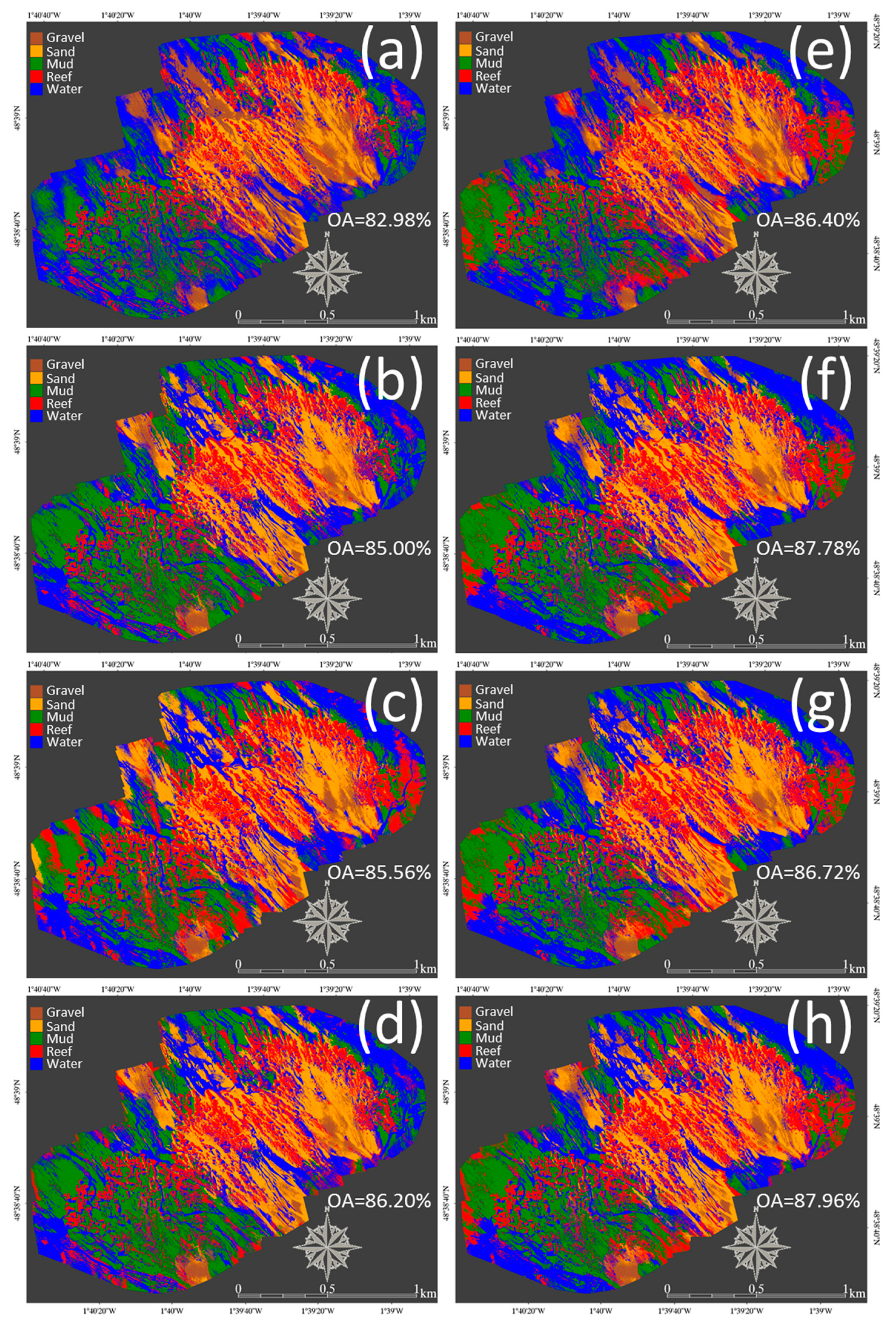
Contributions (in the form of GPs) were described when variables were isolated, on the one hand, and combined, on the other hand, in order to discriminate the inherent effect. Taken separately, the DSM (Figure 4e) drastically augmented the primary RGB classification (3.42%), becoming the best single contributor. The NIR (Figure 4c) and the RE (Figure 4b) both gradually increased the RGB classification by 2.58% and 2.02%, respectively (Table 2). When combined, the best combination increasing the standard RGB classification was the full dataset DSM+RE+NIR (4.98%, Figure 4h), followed by the DSM+RE dataset (4.80%, Figure 4f), the DSM+NIR dataset (3.74%, Figure 4g), and finally the spectral couple RE+NIR (3.22%, Figure 4d).
3.2. Specific Contributions of the DSM, RE, and NIR
The contributions (in the form of GPs) of the spatial DSM and spectral RE and NIR were also investigated at the class level (Figure 5).
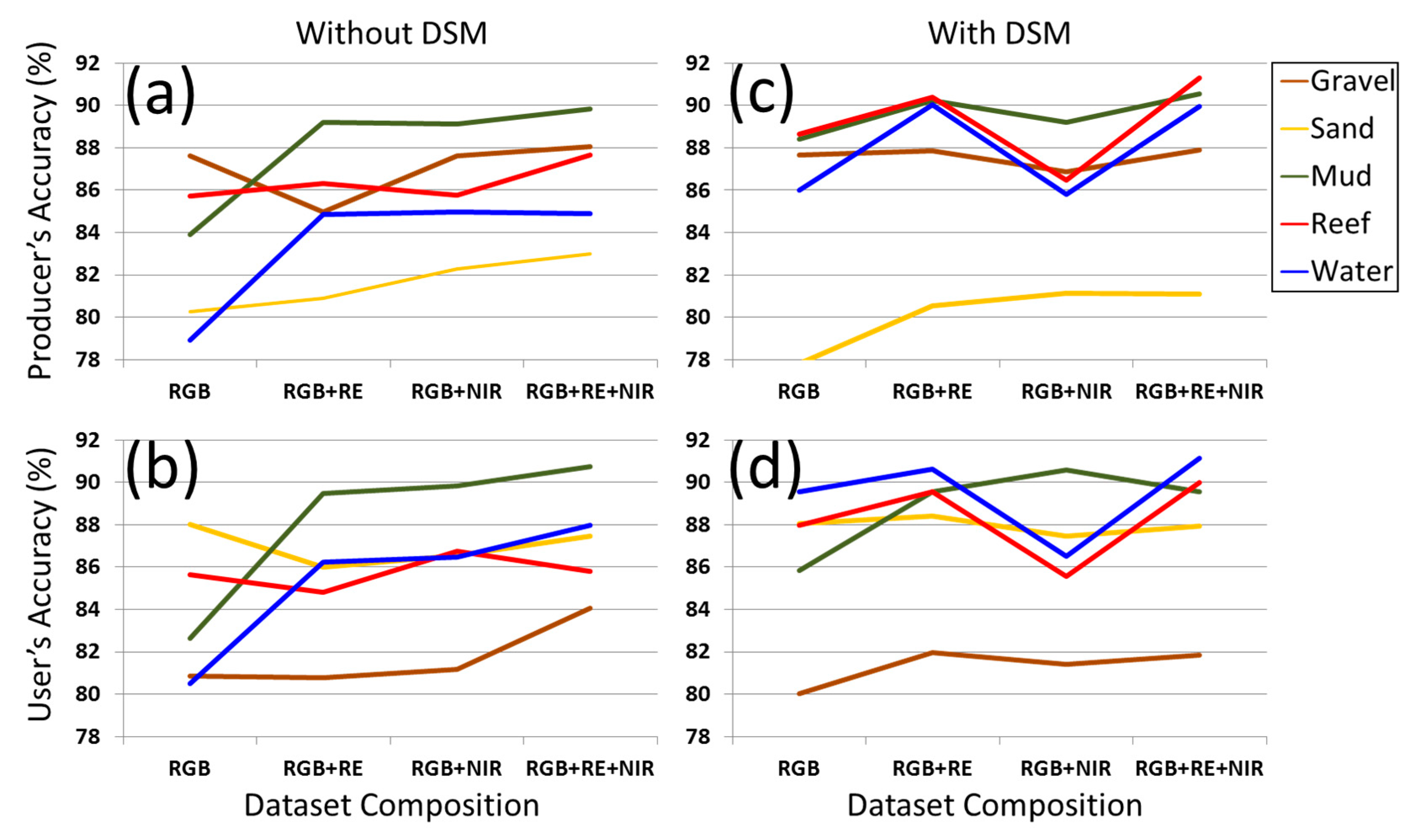
Prior to detailing the effects of DSM, RE, and NIR on the PA and UA of the five classes, gains and losses drawn from average PA+UA were examined to retrieve trends at the class scale. The highest contribution, associated with the full dataset DSM+RE+NIR, increasingly favored sand (0.37%), gravel (0.63%), reef (4.97%), mud (6.79%), and water (10.85%) (Figure 5c,d). The effects of both isolated RE and NIR acted on the same sorting of the five classes: sand (−0.70 and 0.29%, respectively), gravel (−1.35 and 0.15%, respectively), reef (−0.13 and 0.57%, respectively), mud (6.07 and 6.21%, respectively) and water (5.84 and 6.02%, respectively) (Figure 5a,b). This ranking remained constant across the combinations: from the best DSM+RE+NIR, to the lowest RE+NIR, through the DSM+RE and DSM+NIR.
From the viewpoint of the map maker (PA), gravel, reef, sand, mud, and water average classifications were increasingly higher without DSM (Figure 5a), while gravel, sand, reef, mud, and water mean classifications gradually waxed with DSM (Figure 5c). From the viewpoint of the map user (UA), sand, reef, gravel, water, and mud average classifications progressively climbed without DSM (Figure 5b), while sand, gravel, reef, mud, and water were increasingly classified (Figure 5d).
Without DSM, RE increasingly contributed to improve the PA of reef (0.58%), sand (0.63%), mud (5.29%), and water (5.91%), but declined the PA of gravel (−2.66%), while increasing the UA of water (5.76%) and mud (6.84%), but decreasing the UA of gravel (−0.05%), reef (−0.85%), and sand (−2.03%). NIR boosted the PA of reef (0.06%), sand (2.04%), mud (5.23%), and water (6.05%), but reduced the PA of gravel (–0.03%), while augmenting the UA of gravel (0.32%), reef (1.09%), water (6.00%), and mud (7.18%), but diminishing the UA of sand (−1.47%). The joint effect of RE and NIR enhanced the PA of gravel (0.43%), reef (1.93%), sand (2.76%), water (5.95%), mud (5.96%), the UA of reef (0.13%), gravel (3.24%), water (7.49%), and mud (8.09%), but negatively impacted the UA of sand (−0.54%).
With DSM, RE all enhanced the PA of gravel (0.21%), sand (0.30%), reef (4.67%), mud (6.32%), water (11.10%), the UA of sand (0.39%), gravel (1.11%), reef (3.88%), mud (6.90%), and water (10.14%). NIR augmented the PA of reef (0.75%), sand (0.89%), mud (5.30%), water (6.89%), the UA of gravel (0.58%), water (6.01%), and mud (7.96%), while waning the PA of gravel (−0.76%), the UA of reef (−0.09%), and sand (−0.54%). The combined RE and NIR ameliorated the PA of gravel (0.28%), sand (0.84%), reef (5.59%), mud (6.65%), water (11.04%), the UA of gravel (0.99%), reef (4.34%), mud (6.93%), and water (10.65%), but declined the UA of sand (−0.09%).
4. Discussion
4.1. Influence of the Spatial DSM
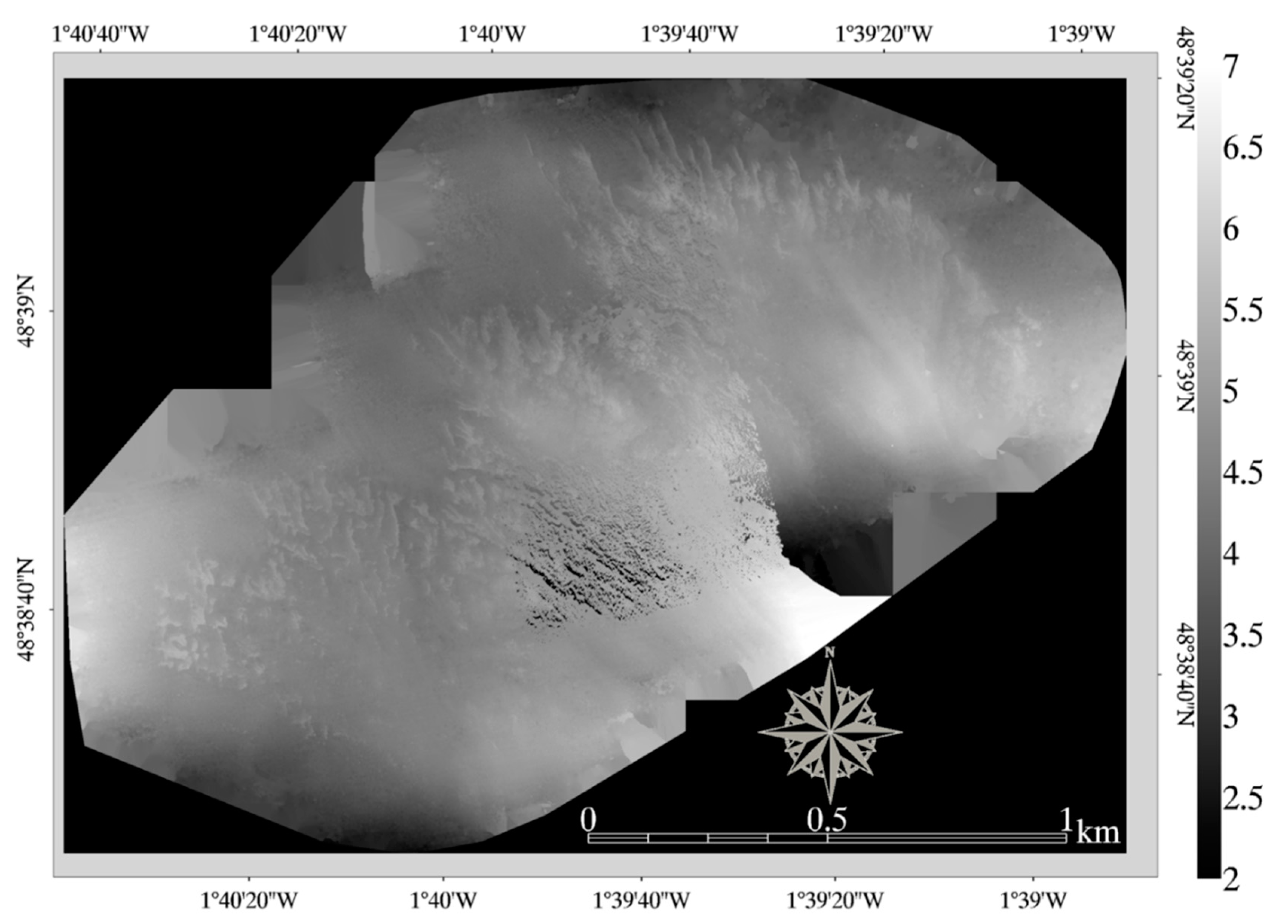
The DSM effect on the RGB reefscape classification (Figure 6) was greater than the contribution of the combined RE and NIR spectral bands. The information related to the elevation and height of reefscape features was therefore more profitable to the classification accuracy than the biophysical properties provided by RE and NIR, namely water content and pigments of these features [10]. Topography is indeed well recognized to be a proximal factor to explain habitat patterns in the intertidal zone [21], given its strong correlation with hydrodynamic, light, and temperature exposure that shape the ecological niches. The ascending contributions of the DSM targeted sand, gravel, reef, mud, and water. The DSM brought insights into the classification of the water and mud classes, which are the topographically-lowest habitats, then the reef class, which is the topographically-highest habitat.
The merge of the DSM with RE+NIR and the DSM with RE were successful for the RGB reefscape classification (highest accuracies), but the fusion of the DSM with NIR did not yield a strong performance. This outcome is corroborated by the examination at the class level: average PA and UA of the five classes leveraged the joint effect of the DSM with RE, while the average PA and UA of gravel were reduced when the DSM and NIR were combined. Characterized by higher wavelengths than these of RE (730–740 nm), NIR (770–810 nm) was much more absorbed by water content [10] and thereafter probably covariated more with elevation and height (i.e., DSM) in the intertidal area. This could have generated statistical noise due to redundant information, thus weakening the correct classification of these two sediment classes. Noteworthy were the differences in average PA and UA gains/losses between the DSM+RE and DSM+NIR: mud (−0.02%), sand (0.16%), gravel (0.75%), reef (3.94%), and water (4.17%). The classification-eroding statistical noise likely to occur for the bottom water and top reef did not considerably play with intermediate gravel, sand, and mud. This finding could be explained by the topographically-median niche occupied by the sediment classes, deprived of the DSM+NIR redundant information. This research hypothesis will be deciphered by statistically testing the difference in average elevation and height of each of the five classes [22].
4.2. Influence of the Spectral RE and NIR
At the reefscape scale, the best spectral contribution, deprived of and provided with the DSM, to the RGB classification was attributed to the joint use of RE and NIR. However, the discrimination derived from the combination of the DSM+RE greatly surpassed this of the DSM+NIR dataset (sooner discussed in Section 4.1).
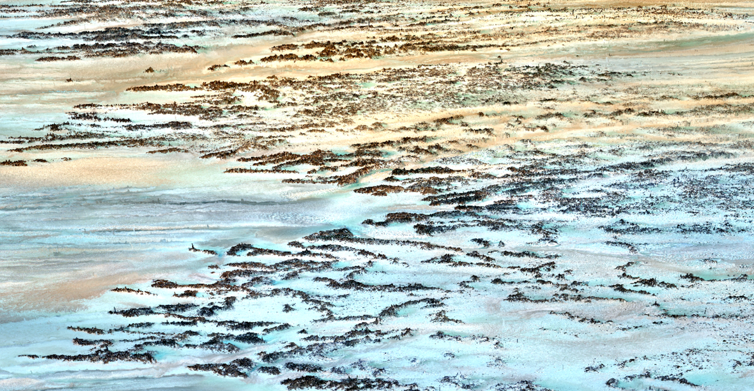
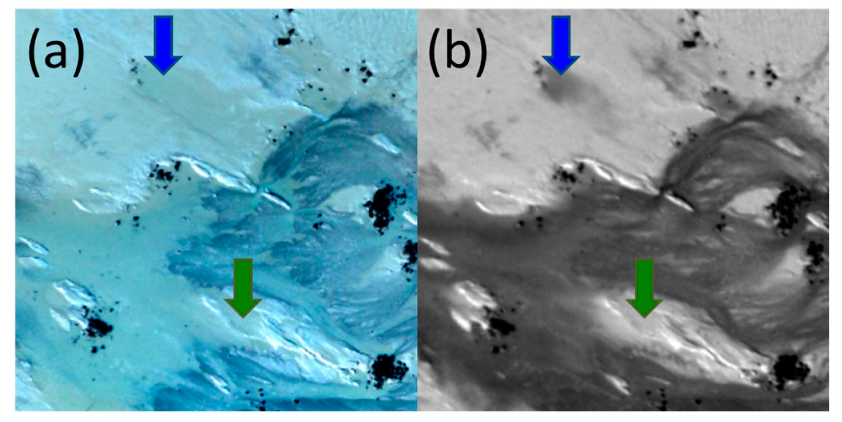
At the class scale, the strong performance of RE+NIR, when deprived of DSM, was easily highlighted by the high gain in both the PA and UA of mud and water classes. The detection of these two classes is directly associated with the water content, which shows a significant signature into the RE and NIR bands [10]. These spectral windows enabled to discriminate mud from water, which were confounded over the natural-colored imagery (Figure 7a), while obviously separable over the NIR imagery (Figure 7b). Of special interest was the gain in both the PA and UA of the reef class. Colonized by sessile oysters, mussels, and, importantly, fleshy seaweed, honeycomb worm reefs might have benefited from the added value of the RE and NIR sensitive, among others, to the chlorophyll pigments [8,23]. Ambivalent contributions of the RE and NIR were found out for the PA and UA of sand and gravel classes, either a positive effect of both RE and NIR for the PA of sand concomitantly with a negative effect for the PA of gravel or the opposite for the UA. Misclassifications of these two sediment classes could be due to two factors: (1) the coarse grain-size making the water content rapidly invisible to the RE and NIR bands at low tide; (2) the potential confusion of these classes, especially the sand, with the reef class, insofar as the worm tubes of the reefs are composed of the same grain-size, despite worm preferences for calcareous versus siliceous materials [24]. A further analysis of the confusion matrices with a careful attention on the sand and reef pixels could unveil this discrepancy.
5. Conclusions
Intertidal bioconstructions of the honeycomb worm reefs were surveyed by a 150 m-height fixed-wings (eBee+®) provided with a multispectral sensor (Parrot Sequoia®). The RGB classification accuracy of the reefscape, examined as a mosaic of five habitats, was improved by the DSM, RE, and NIR information, both separately and jointly.
Separately, the highest overall GP stemmed from the spatial asset DSM (3.42%) derived from the photogrammetric approach, while the best spectral performance was ensured by the NIR spectral band (2.58%), followed by the RE (2.02%). At the class scale, the three DSM, NIR, and RE datasets coincidentally and increasingly advantaged sand, gravel, reef, mud, and water.
Synergistically, the best overall GP relied on the combination of the full dataset (DSM+RE+NIR, 4.98%), followed by the DSM with RE (4.80%), the DSM with NIR (3.74%), and the spectral couple RE with NIR (3.22%). These efficient datasets also profited the same ascending sorting at the class level: sand, gravel, reef, mud, and water. The joint effect of the DSM and NIR produced an overall low gain, compared to the DSM with RE, what was hypothesized to be associated with a statistical noise originated from redundant information in the intertidal area.
As short-term perspectives, the habitat classification will be very likely refined by the integration of spatially- and spectrally-derived products (such as runoff, topographic position index, rugosity index, normalized difference vegetation index, normalized difference water index, etc.) into an object-based image analysis [25].
Author Contributions
Conceptualization, A.C. and T.H.; methodology, A.C. and T.H.; software, A.C. and T.H.; validation, A.C., T.H. and D.J.; formal analysis, A.C.; investigation, A.C., D.J. and T.H.; resources, A.C., D.J., S.D. and T.H.; data curation, A.C. and T.H.; writing—original draft preparation, A.C.; writing—review and editing, A.C., S.D. and T.H.; visualization, A.C. and T.H.; supervision, A.C.; project administration, A.C. and T.H.; funding acquisition, A.C. and T.H.
Funding
This research received no external funding.
Acknowledgments
A.C. acknowledges Camille Ramambason for her 2017 photoquadrat campaign and T.H. is grateful to Gaëtan Palka for his involvement in the 2019 GNSS survey. We also thank Ninon Powers for the proofreading and three anonymous reviewers for the manuscript improvement.
Conflicts of Interest
The authors declare no conflict of interest.
References
- Anders, M.S.; Reid, R.P. Growth morphologies of modern marine stromatolites: A case study from Highborne Cay, Bahamas. Sediment. Geol. 2006, 185, 319–328. [Google Scholar] [CrossRef]
- Gherardi, D.F.M.; Bosence, D.W.J. Composition and Community Structure of the Coralline Algal Reefs from Atol Das Rocas, South Atlantic, Brazil. Coral Reefs 2001, 19, 205–219. [Google Scholar] [CrossRef]
- Naylor, L.A.; Viles, H.A. A temperate reef builder: An evaluation of the growth, morphology and composition of Sabellaria Alveolata (L.) colonies on carbonate platforms in South Wales. Geol. Soc. Lond. Spec. Publ. 2000, 178, 9–19. [Google Scholar] [CrossRef]
- Mumby, P.J.; Skirving, W.; Strong, A.E.; Hardy, J.T.; LeDrew, E.F.; Hochberg, E.J.; Stumpf, R.P.; David, L.T. Remote sensing of coral reefs and their physical environment. Mar. Pollut. Bull. 2004, 48, 219–228. [Google Scholar] [CrossRef] [PubMed]
- Peterson, G.; Harmáčková, Z.; Meacham, M.; Queiroz, C.; Jiménez-Aceituno, A.; Kuiper, J.; Malmborg, K.; Sitas, N.; Bennett, E. Welcoming different perspectives in IPBES: “Nature’s contributions to people” and “Ecosystem services”. Ecol. Soc. 2018, 23, 39. [Google Scholar] [CrossRef]
- Galparsoro, I.; Rodríguez, J.G.; Menchaca, I.; Quincoces, I.; Garmendia, J.M.; Borja, Á. Benthic habitat mapping on the Basque continental shelf (SE Bay of Biscay) and its application to the European Marine Strategy Framework Directive. J. Sea Res. 2015, 100, 70–76. [Google Scholar] [CrossRef] [Green Version]
- Collin, A.; Ramambason, C.; Pastol, Y.; Casella, E.; Rovere, A.; Thiault, L.; Espiau, B.; Siu, G.; Lerouvreur, F.; Nakamura, N.; et al. Very high resolution mapping of coral reef state using airborne bathymetric LiDAR surface-intensity and drone imagery. Int. J. Remote Sens. 2018, 39, 5676–5688. [Google Scholar] [CrossRef] [Green Version]
- Collin, A.; Dubois, S.; Ramambason, C.; Etienne, S. Very high-resolution mapping of emerging biogenic reefs using airborne optical imagery and neural network: The honeycomb worm (Sabellaria alveolata) case study. Int. J. Remote Sens. 2018, 39, 5660–5675. [Google Scholar] [CrossRef]
- Collin, A.; Andel, M.; James, D.; Claudet, J. The superspectral/hyperspatial WorldView-3 as the link between spaceborne hyperspectral and airborne hyperspatial sensors: The case study of the complex tropical coast. Int. Arch. Photogramm. Remote Sens. Spat. Inf. Sci. 2019, XLII-2/W13, 1849–1854. [Google Scholar] [CrossRef]
- Pope, R.M.; Fry, E.S. Absorption spectrum (380–700 nm) of pure water. II. Integrating cavity measurements. Appl. Opt. 1997, 36, 8710–8723. [Google Scholar] [CrossRef]
- Guenther, G.C.; Brooks, M.W.; LaRocque, P.E. New capabilities of the “SHOALS” airborne lidar bathymeter. Remote Sens. Environ. 2000, 73, 247–255. [Google Scholar] [CrossRef]
- Ventura, D.; Bonifazi, A.; Gravina, M.; Belluscio, A.; Ardizzone, G. Mapping and classification of ecologically sensitive marine habitats using unmanned aerial vehicle (UAV) imagery and Object-Based Image Analysis (OBIA). Remote Sens. 2018, 10, 1331. [Google Scholar] [CrossRef]
- Casella, E.; Collin, A.; Harris, D.; Ferse, S.; Bejarano, S.; Parravicini, V.; Hench, J.L.; Rovere, A. Mapping coral reefs using consumer-grade drones and structure from motion photogrammetry techniques. Coral Reefs 2017, 36, 269–275. [Google Scholar] [CrossRef]
- Noernberg, M.A.; Fournier, J.; Dubois, S.; Populus, J. Using Airborne Laser Altimetry to Estimate Sabellaria Alveolata (Polychaeta: Sabellariidae) Reefs Volume in Tidal Flat Environments. Estuar. Coast. Shelf Sci. 2010, 90, 93–102. [Google Scholar] [CrossRef]
- Dubois, S.; Barillé, L.; Cognie, B.; Beninger, P.G. Particle Capture and Processing Mechanisms in Sabellaria Alveolata (Polychaeta: Sabellariidae). Mar. Ecol. Prog. Ser. 2005, 301, 159–171. [Google Scholar] [CrossRef]
- Desroy, N.; Dubois, S.F.; Fournier, J.; Ricquiers, L.; Le Mao, P.; Guerin, L.; Gerla, D.; Rougerie, M.; Legendre, A. The Conservation Status of Sabellaria Alveolata (L.) (Polychaeta: Sabellariidae) Reefs in the Bay of Mont-Saint-Michel. Aquat. Conserv. Mar. Freshw. Ecosyst. 2011, 21, 462–471. [Google Scholar] [CrossRef]
- Plicanti, A.; Domínguez, R.; Dubois, S.; Bertocci, I. Human Impacts on Biogenic Habitats: Effects of Experimental Trampling on Sabellaria Alveolata (Linnaeus, 1767) Reefs. J. Exp. Mar. Biol. Ecol. 2016, 478, 34–44. [Google Scholar] [CrossRef]
- Curd, A.; Pernet, F.; Corporeau, C.; Delisle, L.; Firth, L.B.; Nunes, F.L.; Dubois, S.F. Connecting organic to mineral: How the physiological state of an ecosystem-engineer is linked to its habitat structure. Ecol. Indic. 2019, 98, 49–60. [Google Scholar] [CrossRef]
- Dubois, S.; Commito, J.A.; Olivier, F.; Retière, C. Effects of Epibionts on Sabellaria Alveolata (L.) Biogenic Reefs and Their Associated Fauna in the Bay of Mont Saint-Michel. Estuar. Coast. Shelf Sci. 2006, 68, 635–646. [Google Scholar] [CrossRef]
- Congalton, R.G.; Green, K. Assessing the Accuracy of Remotely Sensed Data: Principles and Practices; CRC Press: Boca Raton, FL, USA, 2008. [Google Scholar]
- Collin, A.; Archambault, P.; Planes, S. Revealing the regime of shallow coral reefs at patch scale by continuous spatial modeling. Front. Mar. Sci. 2014, 1, 65. [Google Scholar] [CrossRef]
- Collin, A.; Long, B.; Archambault, P. Coastal kelp forest habitat in the Baie des Chaleurs, Gulf of St. Lawrence, Canada. In Seafloor Geomorphology as Benthic Habitat; Harris, P.T., Baker, E.K., Eds.; Elsevier: Amsterdam, The Netherlands, 2012; pp. 201–211. [Google Scholar]
- Zacharias, M.; Niemann, O.; Borstad, G. An assessment and classification of a multispectral bandset for the remote sensing of intertidal seaweeds. Can. J. Remote Sens. 1992, 18, 263–274. [Google Scholar] [CrossRef]
- Lisco, S.; Moretti, M.; Moretti, V.; Cardone, F.; Corriero, G.; Longo, C. Sedimentological Features of Sabellaria Spinulosa Biocontructions. Mar. Pet. Geol. 2017, 87, 203–212. [Google Scholar] [CrossRef]
- Collin, A.; James, D.; Jeanson, M.; Claudet, J. Mapping tropical coastal social-ecological systems using unmanned airborne vehicle (UAV). In Proceedings of the Marine Geological & Biological Habitat Mapping (Geohab 2019), Saint Petersburg, Russia, 14 May 2019; Ryabchuk, P., Ed.; Geohab: Saint-Petersburg, Russia, 2019. [Google Scholar]
Figure 1.
Natural-colored drone-based imagery (13,820 × 10,315 pixels with 0.17 m pixel size) of Sainte-Anne honeycomb worm reefs in the Bay of Mont-Saint-Michel (BMSM) (France). The orthomosaic was derived from a 150 m-height eBee+® campaign, carried out on 22 March 2019. Brown, orange, green, red and blue dots correspond to pure gravel, sand, mud, reef, and water ground-truth data, respectively.

Figure 2.
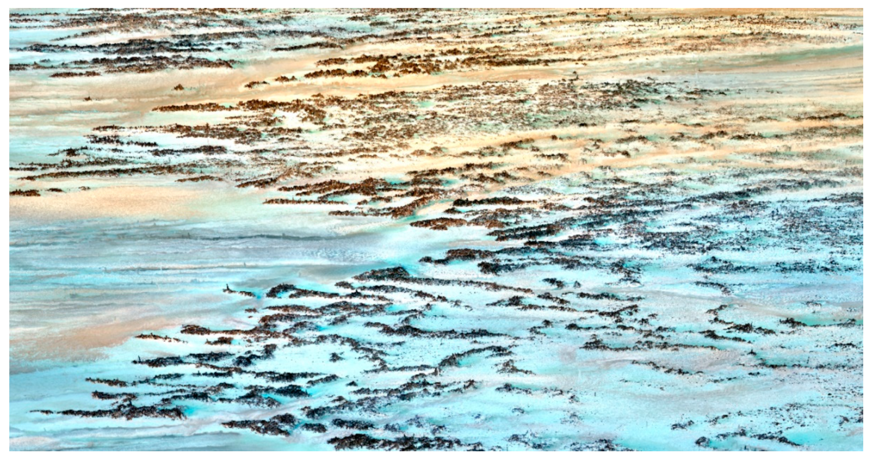
(a) Red edge and (b) near-infrared drone-based spectral reflectance bands (13,820 × 10,315 pixels with 0.17 m pixel size) of Sainte-Anne honeycomb worm reefs in the BMSM (France). The orthomosaic was derived from a 150 m-height eBee+® campaign, carried out on 22 March 2019.
Figure 2.
(a) Red edge and (b) near-infrared drone-based spectral reflectance bands (13,820 × 10,315 pixels with 0.17 m pixel size) of Sainte-Anne honeycomb worm reefs in the BMSM (France). The orthomosaic was derived from a 150 m-height eBee+® campaign, carried out on 22 March 2019.

Figure 3.
Digital surface model (13,820 × 10,315 pixels with 0.17 m pixel size) of Sainte-Anne honeycomb worm reefs in the BMSM (France). The orthomosaic, referenced to the chart datum, was derived from a 150 m-height eBee+® campaign, carried out on 22 March 2019.
Figure 3.
Digital surface model (13,820 × 10,315 pixels with 0.17 m pixel size) of Sainte-Anne honeycomb worm reefs in the BMSM (France). The orthomosaic, referenced to the chart datum, was derived from a 150 m-height eBee+® campaign, carried out on 22 March 2019.

Figure 4.
Classification maps of Sainte-Anne honeycomb worm reefs into five classes: (a) RGB without DSM; (b) RGB+RE without DSM; (c) RGB+NIR without DSM; (d) RGB+RE+NIR without DSM; (e) RGB with DSM; (f) RGB+RE with DSM; (g) RGB+NIR with DSM; and (h) RGB+RE+NIR with DSM.
Figure 4.
Classification maps of Sainte-Anne honeycomb worm reefs into five classes: (a) RGB without DSM; (b) RGB+RE without DSM; (c) RGB+NIR without DSM; (d) RGB+RE+NIR without DSM; (e) RGB with DSM; (f) RGB+RE with DSM; (g) RGB+NIR with DSM; and (h) RGB+RE+NIR with DSM.

Figure 5.
Lineplots of the producer accuracies (PAs) and UAs stemming from the ML classifications of the RGB deprived of (a and b, respectively) and provided with (c and d, respectively) the DSM, both series enriched with isolated and joint RE and NIR spectral bands.
Figure 5.
Lineplots of the producer accuracies (PAs) and UAs stemming from the ML classifications of the RGB deprived of (a and b, respectively) and provided with (c and d, respectively) the DSM, both series enriched with isolated and joint RE and NIR spectral bands.

Figure 6.
Three-dimensional (3D) visualization of the southwestern part of Sainte-Anne honeycomb worm reefscape composed of the RGB imagery draped over the DSM, all derived from a 150 m-height eBee+® survey, carried out on 22 March 2019.
Figure 6.
Three-dimensional (3D) visualization of the southwestern part of Sainte-Anne honeycomb worm reefscape composed of the RGB imagery draped over the DSM, all derived from a 150 m-height eBee+® survey, carried out on 22 March 2019.

Figure 7.
Imageries of Sainte-Anne honeycomb worm reefs showing the spectral confusion of mud (green arrow) and water (blue arrow) in the (a) RGB imagery, while clearly separable in the (b) NIR imagery.
Figure 7.
Imageries of Sainte-Anne honeycomb worm reefs showing the spectral confusion of mud (green arrow) and water (blue arrow) in the (a) RGB imagery, while clearly separable in the (b) NIR imagery.


Table 1.
Description of the five classes used for the mapping. Natural-colored, geometrically-corrected photoquadrats (0.5 × 0.5 m2) correspond to pure classes.
Table 1.
Description of the five classes used for the mapping. Natural-colored, geometrically-corrected photoquadrats (0.5 × 0.5 m2) correspond to pure classes.
| Class | Description | Ground Photographs |
|---|---|---|
| Gravel | Siliceous and calcareous sediment particles of 2–200 mm |  |
| Sand | Siliceous and calcareous sediment particles of 0.06–2 mm |  |
| Mud | Siliceous and calcareous sediment particles of <0.002–0.06 mm |  |
| Reef | Colonies of honeycomb worm Sabellaria alveolata |  |
| Water | Tidal channels and ponds |  |
Table 2.
Overall accuracy (OA) percentage of the resulting maximum likelihood (ML) classifications derived from red-green-blue (RGB) deprived of and provided with the digital surface model (DSM), both series enriched with isolated and joint red edge (RE) and near-infrared (NIR) spectral bands.
Table 2.
Overall accuracy (OA) percentage of the resulting maximum likelihood (ML) classifications derived from red-green-blue (RGB) deprived of and provided with the digital surface model (DSM), both series enriched with isolated and joint red edge (RE) and near-infrared (NIR) spectral bands.
| RGB | RGB+RE | RGB+NIR | RGB+RE+NIR | |
|---|---|---|---|---|
| Without DSM | 82.98 | 85.00 | 85.56 | 86.20 |
| With DSM | 86.40 | 87.78 | 86.72 | 87.96 |
© 2019 by the authors. Licensee MDPI, Basel, Switzerland. This article is an open access article distributed under the terms and conditions of the Creative Commons Attribution (CC BY) license (http://creativecommons.org/licenses/by/4.0/).
Share and Cite
MDPI and ACS Style
Collin, A.; Dubois, S.; James, D.; Houet, T. Improving Intertidal Reef Mapping Using UAV Surface, Red Edge, and Near-Infrared Data. Drones 2019, 3, 67. https://doi.org/10.3390/drones3030067
AMA Style
Collin A, Dubois S, James D, Houet T. Improving Intertidal Reef Mapping Using UAV Surface, Red Edge, and Near-Infrared Data. Drones. 2019; 3(3):67. https://doi.org/10.3390/drones3030067
Chicago/Turabian StyleCollin, Antoine, Stanislas Dubois, Dorothée James, and Thomas Houet. 2019. "Improving Intertidal Reef Mapping Using UAV Surface, Red Edge, and Near-Infrared Data" Drones 3, no. 3: 67. https://doi.org/10.3390/drones3030067