Multi-Sensor Assessment of the Effects of Varying Processing Parameters on UAS Product Accuracy and Quality

Abstract

There is a growing demand for the collection of ultra-high spatial resolution imagery using unmanned aerial systems (UASs). UASs are a cost-effective solution for data collection on small scales and can fly at much lower altitudes, thus yielding spatial resolutions not previously achievable with manned aircraft or satellites. The use of commercially available software for image processing has also become commonplace due to the relative ease at which imagery can be processed and the minimal knowledge of traditional photogrammetric processes required by users. Commercially available software such as AgiSoft Photoscan and Pix4Dmapper Pro are capable of generating the high-quality data that are in demand for environmental remote sensing applications. We quantitatively assess the implications of processing parameter decision-making on UAS product accuracy and quality for orthomosaic and digital surface models for RGB and multispectral imagery. We iterated 40 processing workflows by incrementally varying two key processing parameters in Pix4Dmapper Pro, and conclude that maximizing for the highest intermediate parameters may not always translate into effective final products. We also show that multispectral imagery can effectively be leveraged to derive three-dimensional models of higher quality despite the lower resolution of sensors when compared to RGB imagery, reducing time in the field and the need for multiple flights over the same area when collecting multispectral data is a priority. We conclude that when users plan to use the highest processing parameter values, to ensure quality end-products it is important to increase initial flight coverage in advance.

1. Introduction

Recently, the use of unmanned aerial systems (UASs) has progressed from military to civilian applications such as homeland security, rapid-response disaster surveillance, ecological monitoring, earth science research, and humanitarian observations [1,2]. Steady improvements in small-scale technology have allowed UASs to become an alternative remote sensing platform offering on-demand high-resolution data at inexpensive rates [3]. High-resolution imagery collected by UASs can be used to produce high-density point clouds generated by image matching and photogrammetric techniques that rival similar Light Detection and Ranging (LiDAR) platforms for a fraction of the cost [4]. UAS users also have greater control over the temporal scale at which they can collect data, rather than relying on the schedules of airplane pilots and satellites.

The ubiquity and relatively-low cost of UASs and the ever-increasing types of applications and questions that can benefit from the use of UASs has resulted in a growing demand for the collection of these ultra-high spatial resolution data across many platforms and sensor types (visible, multispectral, thermal, LiDAR imagery). The proliferation of data has resulted in rapid advances in imagery processing with commercial software, making algorithms faster and more user-friendly compared to more traditional methods of aerial stereophotogrammetry. Commercially available software such as AgiSoft Photoscan and Pix4Dmapper Pro are capable of generating the high-quality products that are in demand for environmental remote sensing applications. Despite the ubiquity and relatively “canned workflows”, new users often have little previous experience with imagery processing and thus, make processing decisions that may have important implications on their resulting products, often with limited awareness. Even experienced users may make choices in their parameterization without understanding the implications of their decision-making on the final products generation. To our knowledge, no literature exists that quantitatively assesses the effects of making small, incremental variations in some of the key processing parameters in structure-from-motion photogrammetric processing workflows and how those affect resulting UAS imagery-derived products. Gross and Heumann [5] report what they consider to be the optimal parameters for processing UAS-collected imagery in multiple software systems based on reviews of user’s manuals and “trial and error,” but do not provide an in-depth analysis and discussion of parameterization over the full range of options within each software system. In many cases, parameterization may be context-specific, where some parameter values may be more suitable for certain land-use types than others, thus the parameters suggested in Gross and Heumann [5] may be ill suited for application across disparate types of projects.

Our research quantitatively and qualitatively assesses the effects of varying two key processing parameters in the structure-from-motion processing workflow, specifically the keypoint image scale and image scale used in point cloud densification, on the resultant point clouds, orthomosaics, and digital surface models using Pix4Dmapper Pro by Pix4D (hereon referred to as Pix4D) [6]. Previous UAS work by Frasier and Congalton [7] over a forested plot at different flight heights using RGB (SenseFly S.O.D.A. sensor) and multispectral (the Parrot Sequoia sensor) platforms conducted image processing in both Pix4D and Agisoft. However, they only used a singular keypoint image scale and image scale for point cloud densification parameter setting in Pix4D for their comparison. Those choices were made to reduce scene complexity while extracting visual information and to further simplify raw image geometry while computing 3D coordinates, and they noted that those two parameter selections would lead to faster processing in complex landscapes but could influence accuracy. However, they did not investigate the degree and magnitude of changes in accuracies in the resulting derived products. Sona et al. [8] also compared outputs from multiple imagery processing software packages and found AgiSoft Photoscan to perform the best overall; however, the authors did not state explicitly what parameter values they used or why they had chosen them. They did note that when comparing Pix4D and AgiSoft, the former identified fewer matching points than the latter, but Pix4D was able to detect points visible in more images. Furthermore, most studies conducting product accuracy comparisons among software and processing workflows tend to primarily focus on assessing geometric accuracies with little to no indication of what actual processing parameters were used or how and why specific ones were chosen [5,8,9].

Our overarching research question was “how does the choice of processing parameters during the structure-from-motion image processing workflow affect intermediary and final photogrammetric outputs from visible and multispectral imagery and how reliably can multispectral imagery be used to create three-dimensional objects compared to RGB despite significant spatial resolution differences?” We specifically assess the effect of varying the keypoint image scale through all available settings in the leading UAS imagery processing software (Pix4Dmapper Pro) and of simultaneously varying image scale for point cloud densification settings on multiple variables including the calibrated image percent, median number of matches per calibrated image, the number of 2D and 3D keypoints observed for bundle block adjustment, mean image reprojection error, the number of 3D densified points and average point density. We present quantitative assessments and corresponding image-based visualizations during intermediary and final UAS product generation for both visible and multispectral imagery collected using a fixed-wing professional mapping small UAS. Finally, we quantitatively assess the differences between multispectral and RGB imagery to determine whether multispectral imagery, though significantly less detailed in terms of spatial resolution (ground sampling distance) typically, can be considered a reliable source for three-dimensional surfaces such as digital surface and digital terrain models.

2. Background

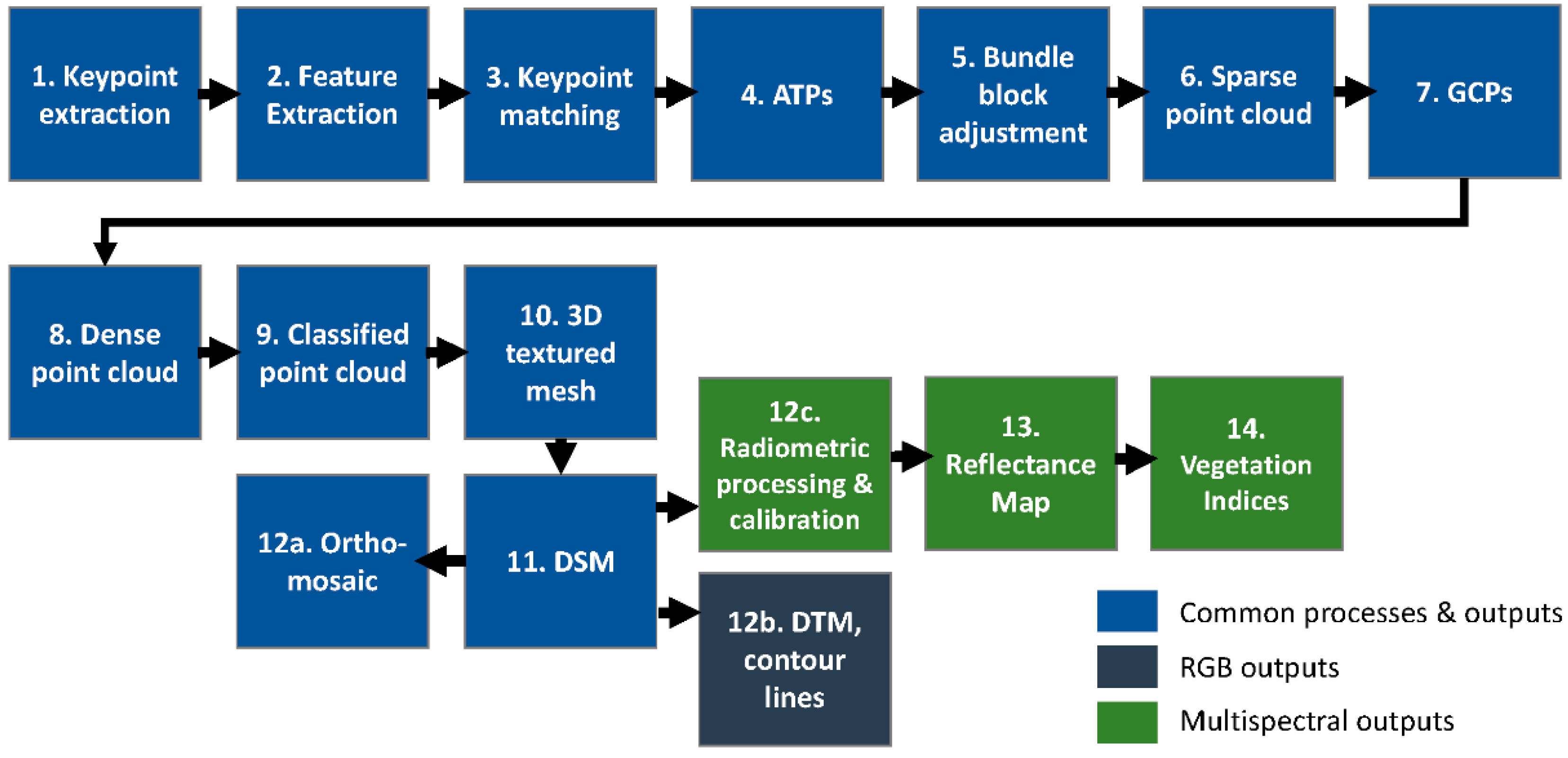
Pix4D uses a modified structure-from-motion, or SFM, approach to process UAS imagery (Figure 1). SFM is a photogrammetric technique used to estimate the three-dimensional (3D) structure of objects from multiple two-dimensional (2D) offset image sequences resulting from the motion of a camera mounted on platforms such as UASs [10]. The initial stages of the process begin with feature extraction and the identification and matching of keypoints, or spatial locations or points in the image that are highly distinctive or stand out in the image. Keypoints are distinctive because no matter how the image is rotated or scaled, the same keypoints have a high probability of identification from a large database of features and many images [11].

There are several algorithms that can be used for keypoint matching and feature extraction such as the Scale-Invariant Feature Transform (SIFT) [11], Speeded-Up Robust Features (SURF) [12], Binary Robust Invariant Scalable Keypoints (BRISK) [13], among others. Given the proprietary nature of Pix4D, the specific feature extraction algorithm used by the software is unknown by users. In Pix4D, the user may identify the keypoint image scale, or the image size at which keypoints are extracted. The values for this parameter range from one-eighth (¹/₈) to two (2). When selecting a keypoint image scale below the original image size, the user can expect a reduction in accuracy because in general, fewer keypoints matched are computed. A decrease in the number of keypoints matched means that there is less confidence of placing a point correctly, whereas more matches means a higher degree of confidence.

A tie point is a specific location that is recognizable in the overlap area between multiple images. Automatic tie points (ATPs) are 3D points that correspond to an automatically detected keypoint and subsequently matched in the images, and allowing the computation to progress from image space to object space. ATPs do not have known ground coordinates but instead, identify relationships between images and are also used in the calibration of images. ATPs and ground control points (GCPs) are then used in the bundle block adjustment (BBA) before the low-density point cloud (LDPC) is constructed. In Pix4D, the BBA is calculated using the relationship between overlapping images, keypoints, and GCPs, and the specific internal camera parameters and adjustments are applied to images within each specific block.

After the generation of the LDPC, the high-density point cloud (HDPC) is created based on the image scale defined by the user. Image scale defines the scale in relation to the original image size at which additional 3D points are generated. In Pix4D, the values for image scale range from one-eighth (¹/₈) to full (1), in ¼ increments.

The final processing steps in Pix4D include the generation of the 3D textured mesh (a triangular surface overlaid on the HDPC), surface models including the digital surface model (DSM) and digital terrain model (DTM), and the orthomosaic. The orthomosaic is obtained from the DSM and corrected for perspective, with the value of each pixel calculated as an average of the pixels in the corresponding original images. All aforementioned steps are applicable to processing both RGB and multispectral imagery. With multispectral imagery processing, the user may create additional reflectance layers, as well as compute indices such as the Normalized Difference Vegetation Index (NDVI).

3. Materials and Methods

3.1. Imagery Collection

Imagery for this project was collected at a location in Brunswick County, North Carolina, USA (Figure 2) using a SenseFly eBee Plus fixed-wing UAS with an onboard real-time kinematics (RTK) receiver. RGB imagery was collected with a SenseFly S.O.D.A. camera (20 megapixels) and multispectral imagery (green, red, red-edge, and near-infrared) was collected using a Parrot Sequoia sensor (1.2 megapixels for the multispectral bands) (

Table 1. Table summarizing the theoretical number of total effective pixels, or pixels available for keypoints extraction, based on sensor type, overlap, and keypoint scale. The values do not represent the actual number of pixels used in the calculations but instead, represent the dimensionality of RGB vs. multispectral imagery.

			Total Pixels Used in Each Keypoint Scale
Camera (Overlap)	Spatial Resolution	Total Pixels	1/8 Image	1/4 Image	1/2 Image	1 Image	2 Image
SODA (70%/65%)	5472 × 3648	19,961,856	2,495,232	4,990,464	9,980,928	19,961,856	39,923,712
Sequoia (60%/80%)	1280 × 960	1,228,800	153,600	307,200	614,400	1,228,800	2,457,600
Camera	% Effective Pixels Compared to SODA			Imagery Data Dimensions		Possible Unique Values
SODA	100%			RGB (255 × 3)		16,581,375
Sequoia	6.16%			Greyscale (65,520 × 1)		65,520

). We used the eMotion flight planning software [14] for all phases of flight planning and management. The same automatic flight mapping mission block was used for both RGB and multispectral flights to ensure imagery collection occurred within the exact flight block for both missions. RGB imagery was collected at a 70% lateral and 65% longitudinal overlap, and multispectral imagery at a 60% lateral and 80% longitudinal overlap. The ground sample distance (GSD), based on a flight altitude of 119 m (400 ft) above mean sea level for both flights, was expected to be 2.9 cm/pixel for RGB and 13.0 cm/pixel for multispectral.

3.2. Imagery Processing

Pix4D v. 4.0.21 was used for all imagery processing [6]. The full range of parameter values were varied simultaneously for both keypoint image scale and image scale used for point cloud densification (

Table 2. Processing iterations used to examine effects of varying keypoint image scale and image scale for point cloud densification for RGB and multispectral imagery in Pix4Dmapper Pro.

	Image Scale for Point Cloud Densification
Keypoint Image Scale	1/8	1/4	1/2	1
1/8	1/8, 1/8	1/8, 1/4	1/8, 1/2	1/8, 1
1/4	1/4, 1/8	1/4, 1/4	1/4, 1/2	1/4, 1
1/2	1/4, 1/8	1/2, 1/4	1/2, 1/2	1/2, 1
1	1, 1/8	1, 1/4	1, 1/2	1, 1
2	2, 1/8	2, 1/4	2, 1/2	2, 1

). All other parameter values were kept constant throughout all of the iterations.

Upon completing the 40 processing iterations on the RGB and multispectral imagery, several metrics from each of the resulting quality reports that relate to the two parameters of interest were extracted and analyzed statistically to assess differences in metric values resulting from parameter value variation (

Table 3. Metrics used to assess quality and accuracy of outputs with varying parameter inputs for RGB and multispectral imagery. Descriptions of metrics are also available at https://support.pix4d.com/hc/en-us/articles/202558679-Quality-report-specifications.

Abbrv	Assessment Metric	Description
CalImg%	Calibrated Image Percent	Percent Images Successfully Calibrated
MedMatch	Median Matches per Calibrated Image	Median number of matched 2D keypoints per image. A matched point is a characteristic point that has initially been detected on at least two images (a 2D keypoint on these images) and has been identified to be the same characteristic point.
2DKP	Number of 2D Keypoints Observed for Bundle Block Adjustment	The number of automatic tie points on all images that are used for the AAT/BBA. It corresponds to the number of all keypoints (characteristic points) that could be matched on at least two images.
3DKP	Number of 3D Points for Bundle Block Adjustment	The number of all 3D points that have been generated by matching 2D points on the images.
MRE	Mean Reprojection Error [pixels]	The average of the reprojection error in pixels. Each computed 3D point has initially been detected on the images (2D keypoint). On each image, the detected 2D keypoint has a specific position. When the computed 3D point is projected back to the images, it has a re-projected position. The distance between the initial position and the re-projected one gives the re-projection error.
3DDP	Number of 3D Densified Points	Total number of 3D densified points obtained for the project.
PtDens	Average Density (m3)	Average number of 3D densified points obtained for the project per cubic meter.

).

3.3. Statistical and Spatial Analyses

Statistical tests were conducted using R 3.4.3 [15] and the corrplot (v0.84) package [16]. Graphs were created using R 3.4.3 [15], the corrplot [16] and the plot3D (v1.1.1) packages [17]. Visual quality assessment of orthomosaics and DSMs was performed in ArcMap (version 10.5.1) [18], while quality assessments of the point cloud used Pix4D [6].

We used an exploratory two-sample t-test to compare metrics generated from RGB processing trials to metrics from multispectral processing trials. These metrics include CalImg%, MedMatch, 2DKP, 3DKP, KRE, 3DDP, and PtDens (see Table 3 for descriptions). The two-sample t-test determines if the means between two groups are statistically different (Equation (1)).

$$t=\frac{{\overline{x}}_1-{\overline{x}}_2-\Delta }{\sqrt{\frac{s_1^2}{n_1}+\frac{s_2^2}{n_2}}}$$

(1)

where ${\overline{x}}_1$ and ${\overline{x}}_2$ are the means of the two samples, Δ is the hypothesized difference between the population means (in this case, 0 because we are testing for equal means), s₁ and s₂ are the standard deviations of the two samples, and n₁ and n₂ are the sizes of the two samples. The number of degrees of freedom (df) for the problem is the smaller of n₁ − 1 and n₂ − 1. We set the significance level for all statistical tests at p = 0.05.

Correlation between metrics was calculated using the corrplot package [16]. This package is used to calculate a correlation matrix and allows the user to create a customized graphical representation of the correlation matrix. The correlation matrix can be displayed in a variety of ways, most of which use a two-hued color map of varying lightness, where the color increases in intensity as the correlation value moves away from zero [19].

Additional visual qualitative and quantitative assessments of imagery and final product comparisons were performed in ArcMap [18]. The boundary of each final orthomosaic was manually digitized to allow us to compare areal extents of orthomosaics as it related to the degree of success of the Pix4D image calibration process. DEMs were visualized using graduated color maps that indicate the range of elevation in each scene.

4. Results and Discussion

Our overarching goal was to understand how the choice of processing parameters during standard structure-from-motion photogrammetric imagery processing workflow influences final outputs (orthomosaics and derived DSM). Using an exploratory two-sample t-test to compare metrics generated from RGB imagery processing trials to metrics from multispectral processing trials over the exact same areal extent of collection, we determined that all variables of comparison are statistically different from one another except for the resulting number of 2D keypoints (2DKP). This indicates that, for the same areal extent and constant altitude of imagery collection, the major quantitative metrics of interest (calibrated image percent, median number of matches per calibrated image, the number of 3D keypoints observed for bundle block adjustment, mean image reprojection error, the number of 3D densified points and average point density) vary significantly between RGB and multispectral imagery collection (

Table 4. Two-sample t-tests results comparing metrics from RGB and multispectral imagery processing (refer back to Table 3 for a description of each metric).

	CalImg%	MedMatch	2DKP	3DKP	MRE	3DDP	PtDens
t	2.35	4.05	0.54	3.08	−1.79	3.24	3.54
df	24.97	19.54	21.70	22.99	32.80	19.38	19.07
p-value	0.03	0.00	0.59	0.01	0.08	0.00	0.00

), as would be expected based on the differences in spatial resolution and total number of pixels available for calculating these metrics. The actual GSD and geolocation error values are presented in

Table 5. Average ground sample distance (GSD) and average root mean square (RMS) absolute geolocation error measurements of processed imagery. These numbers were computed as the average among all iterations; thus, we also show standard deviation.

	Expected GSD (cm/px)	Actual GSD (cm/px)	X Error (%)	Y Error (%)	Z Error (%)
RGB	2.9	2.61 (±0.01)	0.02 (±0.01)	0.01 (±0.01)	0.04 (±0.02)
Multispectral	13.0	8.48 (±0.07)	1.42 (±0.32)	1.53 (±0.34)	2.03 (±0.33)

.

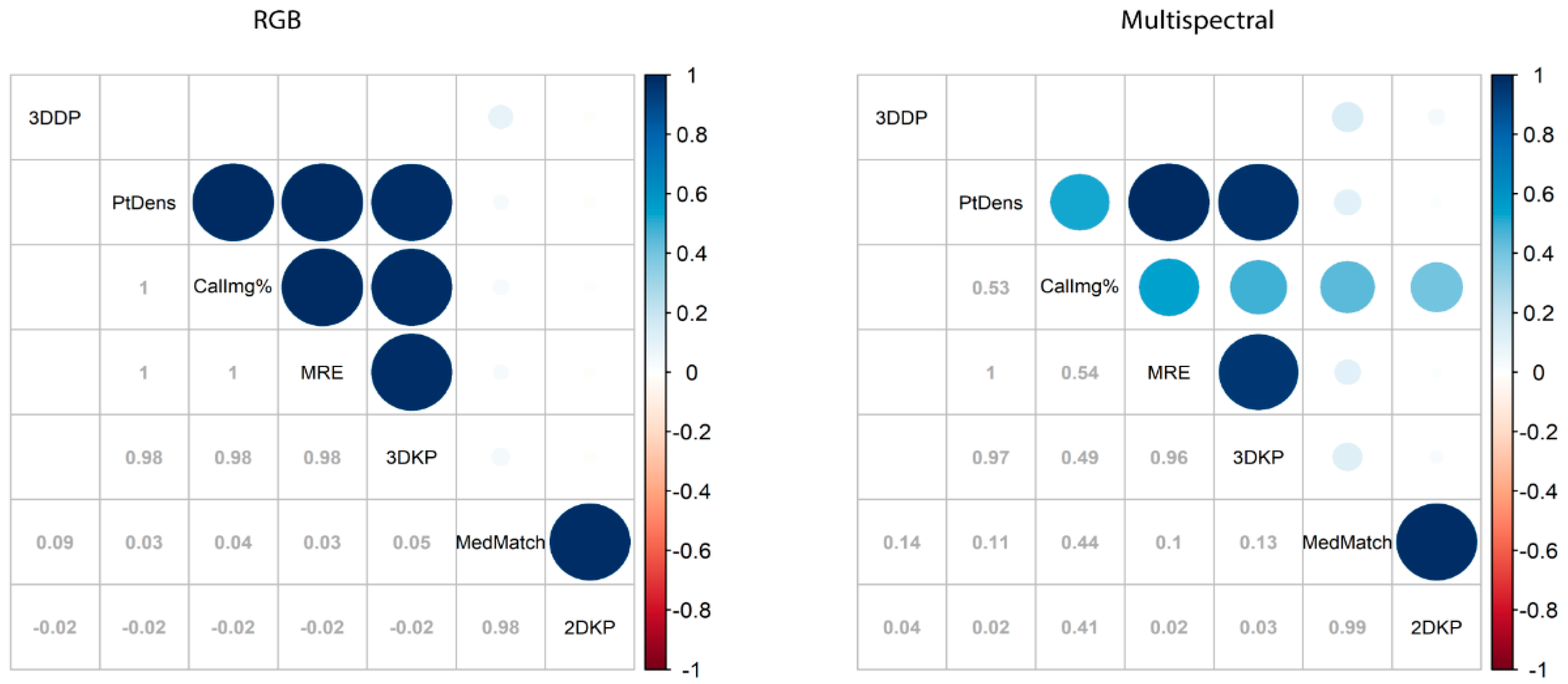
To understand how processing parameter choice affects intermediary product generation (i.e., the metrics listed in Table 4 and Supplementary Materials Tables S1 and S2) we compare: (1) effects within RGB and multispectral imagery individually; and (2) effects between RGB and multispectral imagery. We performed correlation analyses and present results as a correlogram (Figure 3) and discuss only results that were statistically significant (p = 0.05). We found that the number of median matches (MedMatch) and 2D densified keypoints (2DKP) are perfectly correlated (0.99, Figure 3) for both RGB and multispectral imagery, which is to be expected given that these metrics are both derived from the number of 2D keypoints computed. We also observed similar correlations between total point density (PtDens) and the number of 3D points used in the bundle block adjustment (3DKP), which had high correlation values of 0.98 for RGB and 0.97 for multispectral (Figure 3). Similarly, we found that 3DKP and the mean reprojection error (MRE) were almost perfectly correlated (0.98 for RGB and 0.96 for multispectral, Figure 3). There were also some parameter combinations that did not exhibit the same degree of correlation in both RGB and multispectral, such as: calibrated image percent and point density (1 for RGB and 0.53 for multispectral), calibrated image percent and 3DKP (1 for RGB and 0.54 for multispectral), calibrated image percent and median matches (0.05 for RGB and 0.44 for multispectral), and calibrated image percent and 2DKP (0.03 for RGB and 0.41 for multispectral).

When considering 3D relationships, we observed that there is a weak relationship between the number of 3DDP and most other variables, including the percent calibrated images in both RGB and multispectral data. However, 3DDP is significantly weakly correlated with the number of median matches (0.09 for RGB and 0.14 for multispectral, Figure 3), which means that the number of 2DKP potentially plays the biggest role in determining the number of final 3DDP. This means that to maximize 3DDP without significant losses in the effective area covered during processing, flight footprints must be increased during mission planning. One interesting finding is that, despite the high correlation between percent calibrated images and MRE and percent calibrated images and 3DDP for RGB imagery processing (1 and 0.98, respectively), the same relationships were not observed for multispectral imagery (Figure 3). The implication is that regardless of how many calibrated images may exist for a given flight area, a much higher number of 2DKP can be extracted in RGB relative to multispectral imagery. However, high image calibration is critical to ensuring the highest number of 2DKP are generated in any given set of imagery.

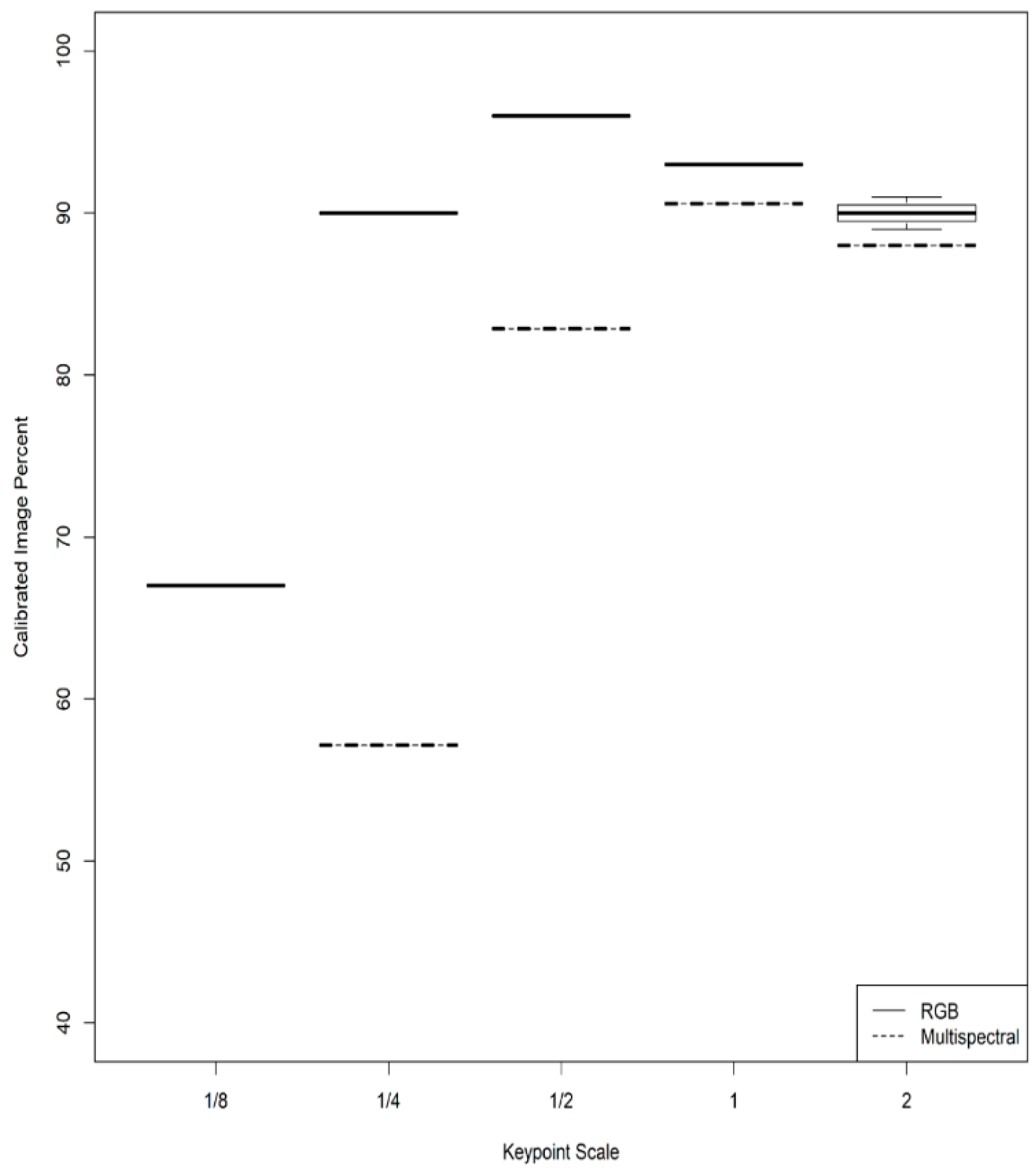
For both RGB and multispectral, we observed a similar pattern in terms of the percent calibrated images: image calibration peaked (at ½ keypoint scale for RGB and full (1) for multispectral), after which, calibrated image percent declined (Figure 4). The variation in percent calibrated images, in turn, affected the final areal extent of the orthomosaic generated because areas with poor calibration were excluded (Figure 2 and Table 1). At most keypoint scales, varying the image scale had no effect on the percent of calibrated images (i.e., the percent of calibrated images was the same at all image scales when keypoint scale remained constant; Figure 4). An exception occurred at two (2) keypoint scale using RGB imagery, where there is a slight variation between the different processing iterations as the image scale was varied. It is possible that this is not due to variation in image scale alone and may occur due to internal variation within the algorithm used by Pix4D. The patterns we observed mimic a diminishing returns function because the calibration will be computationally intensive and result in a lower calibration (Figure 4). This may be especially noticeable for landscapes that are heavily vegetated or very homogeneous due to the limited number of available 2DKP that can be extracted from the imagery.

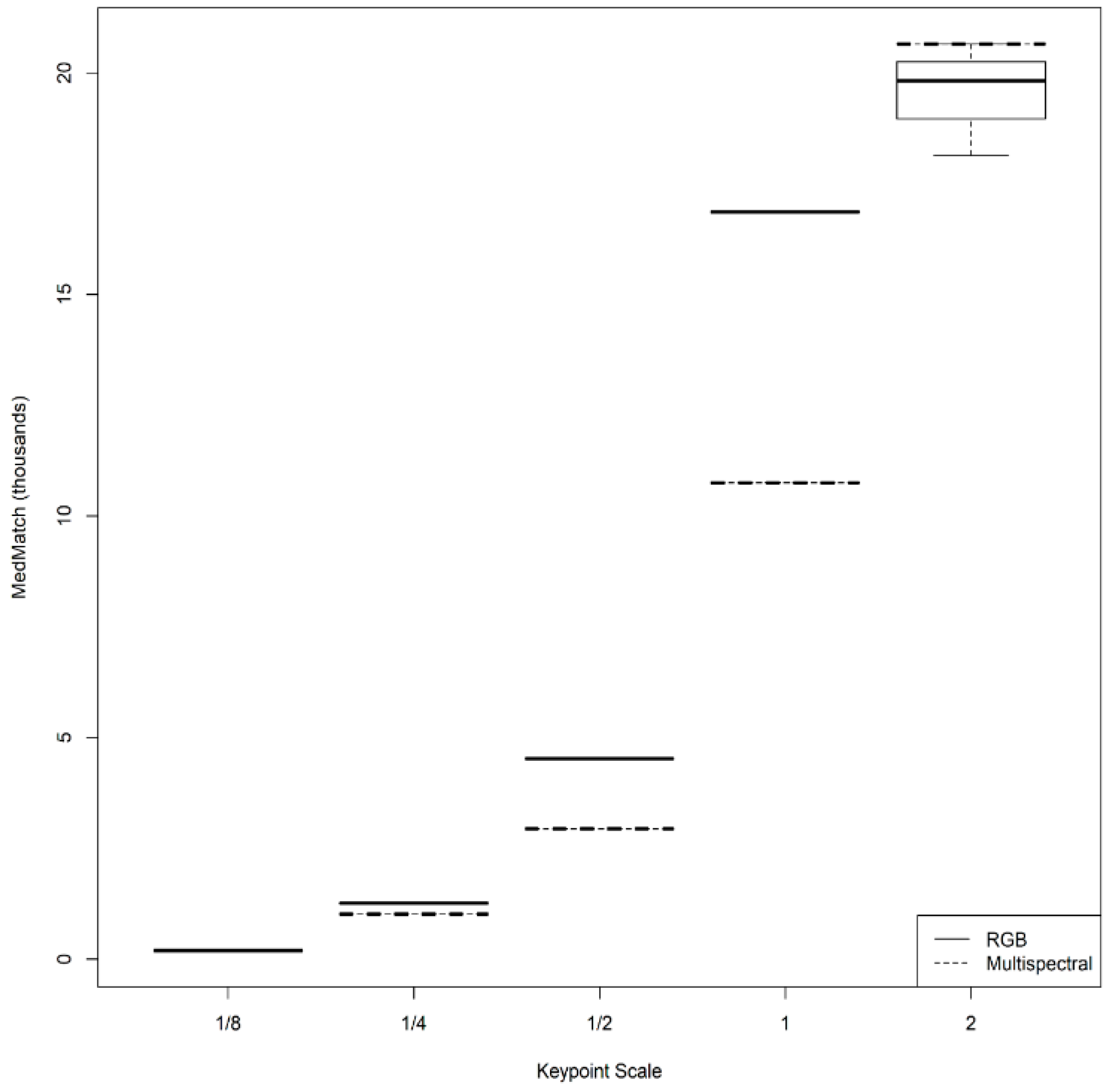
A higher number of median matches for RGB over multispectral imagery was observed for all keypoint image scales except for two (2) where multispectral was higher that RGB, and 1/8 image scale for multispectral imagery where processing failed. There was some variation at two (2) keypoint scale for RGB depending on the image scale for point cloud densification, which is the only instance where there was variation. The patterns we observed mimic an exponential growth curve (Figure 5), and while it is true that a higher number of median matches can be achieved with a higher keypoint scale, computational time will also increase. 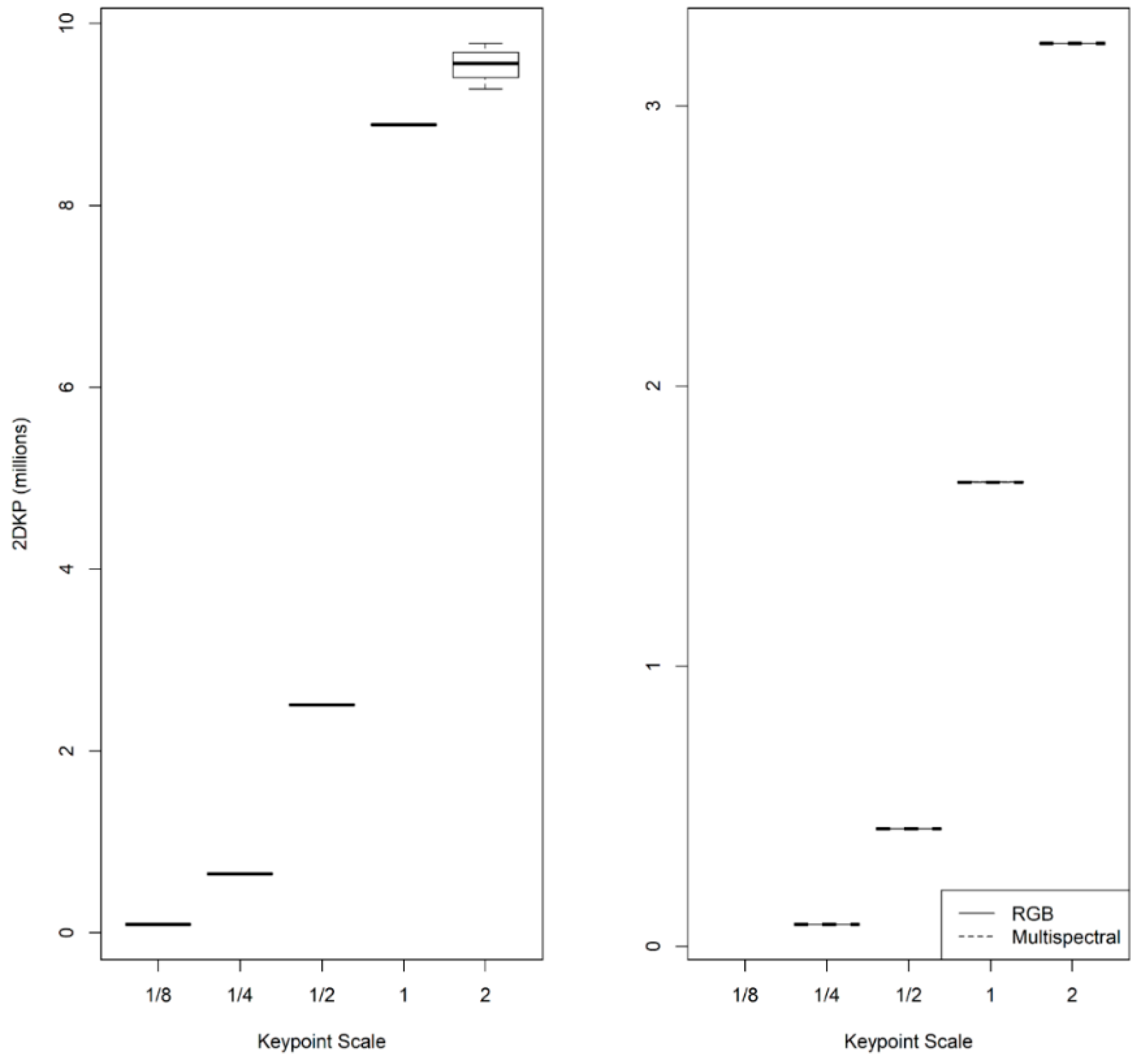Additionally, the calibrated image percent will be lower at two (2) keypoint scale so the increase in number of median matches would actually be made among fewer images (Figure 4 and Figure 5). Likewise, this is true for 2DKP, where we observe the greatest number at two (2) keypoint scale despite lower overall calibration. RGB trials resulted in more 2DKP (in millions) by roughly three orders of magnitude, observed at all keypoint image scales relative to multispectral processing trials (Figure 6). The higher number of matches and 2DKP at two (2) keypoint scale would not compensate for the lost aerial coverage of the final orthomosaic and DSM if critical areas were not included in the calibration. The best results in this context occurred at one (1) keypoint scale, which is the Pix4D default processing value for keypoint scale. However, if initial imagery collection extends slightly outside the area of interest, the longer computation time and decrease in calibration may be a worthwhile tradeoff to maximize extraction of median matches and 2DKP (and thus, also 3DDP, given its previously discussed dependence on 2DKP) in the remaining imagery.

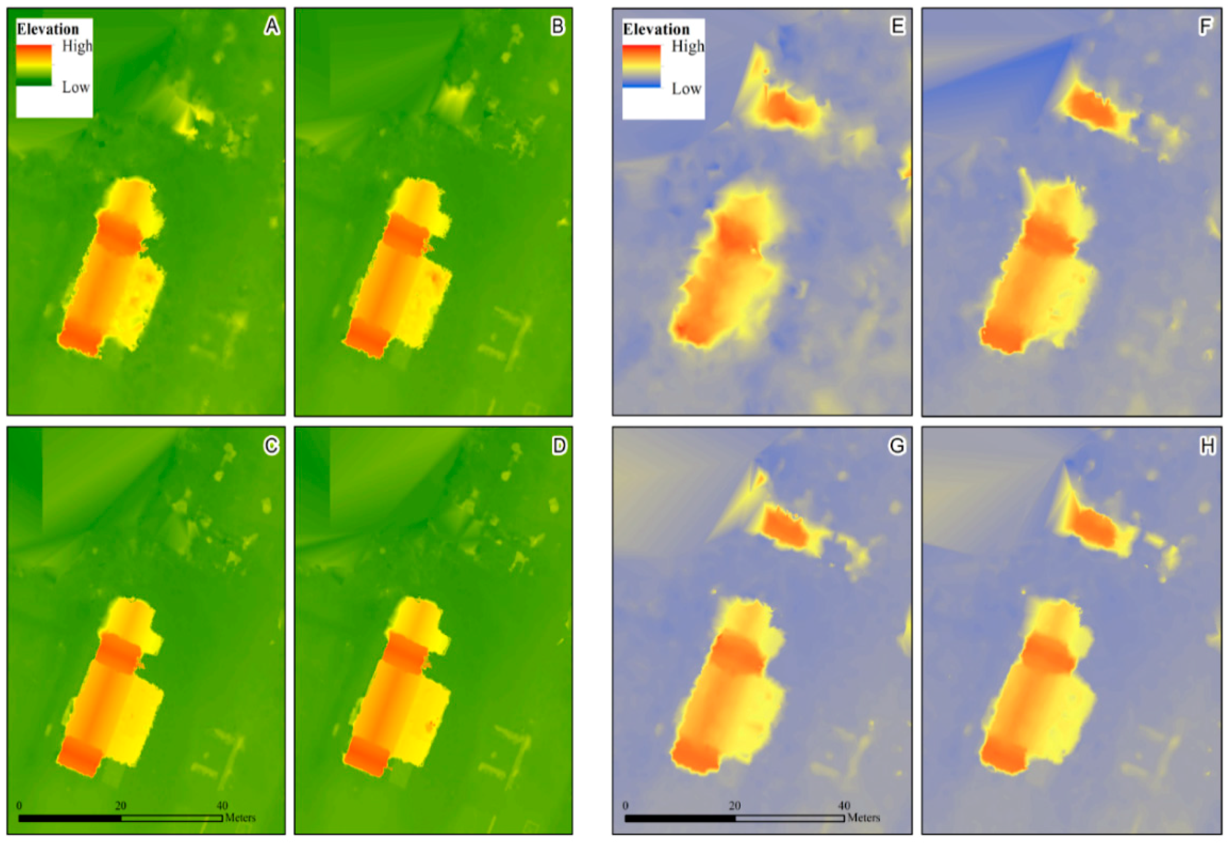
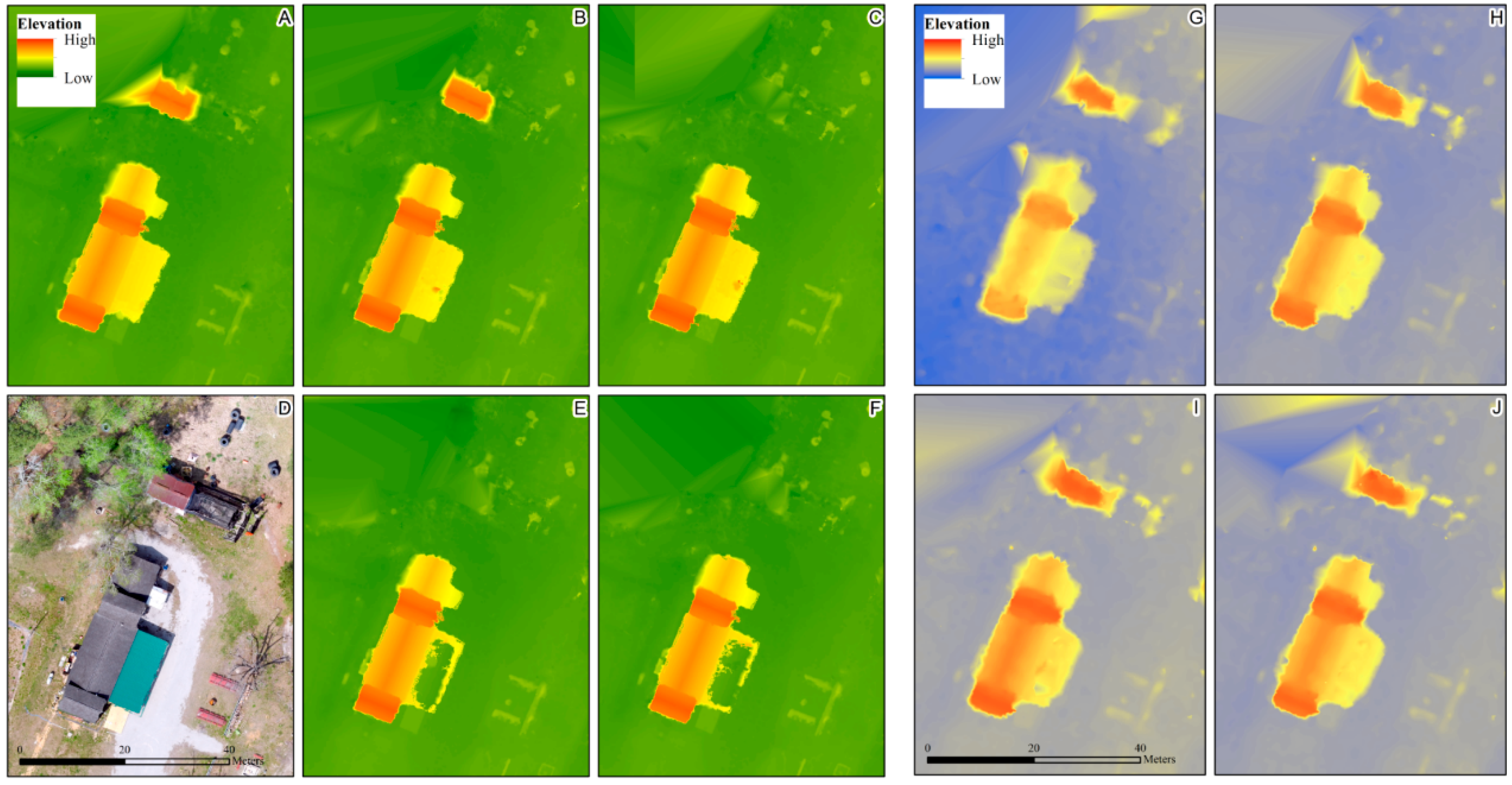
In terms of how keypoint image scale choice translates into spatially defined products such as DSMs, we examined variation in the DSMs when keypoint image scale was varied and image scale for point cloud densification was held constant at full (1). We present important differences between RGB and multispectral trials, as well as within RGB and multispectral trials (Figure 7A–J). Specifically, a building with a red roof (Figure 7D) was visible at 1/8 and 1/4 keypoint scale for RGB but not visible at higher keypoint scales (Figure 7; Figure 2 Area A). This same red building was able to be interpreted at all keypoint scales in multispectral processing trials despite the lower ground sampling distance and pixel size of the imagery. At higher keypoints scales in RGB, Pix4D was less likely to interpret the height of the blue overhang (Figure 7D) correctly. At 1/2 and higher keypoint scales, the Pix4D algorithm’s calculations would also include values from the area below the overhang, leading to the production of a DSM that blends the ground and canopy due to an insufficient number of values being detected for each area individually. Interestingly, a building with a dark roof adjacent to the red building (Figure 7D) does not show up in any of the RGB DSMs and is barely noticeable in the multispectral DSMs. In summary, multispectral data appears to perform better than RGB strictly in terms of detecting buildings or objects with well-defined edges and boundaries that are elevated above ground (Figure 7). This is an interesting finding given the exponentially higher frequency with which RGB imagery is used to produce DSMs compared to multispectral imagery and points to an under-studied area within the broader umbrella of the UAS sciences.

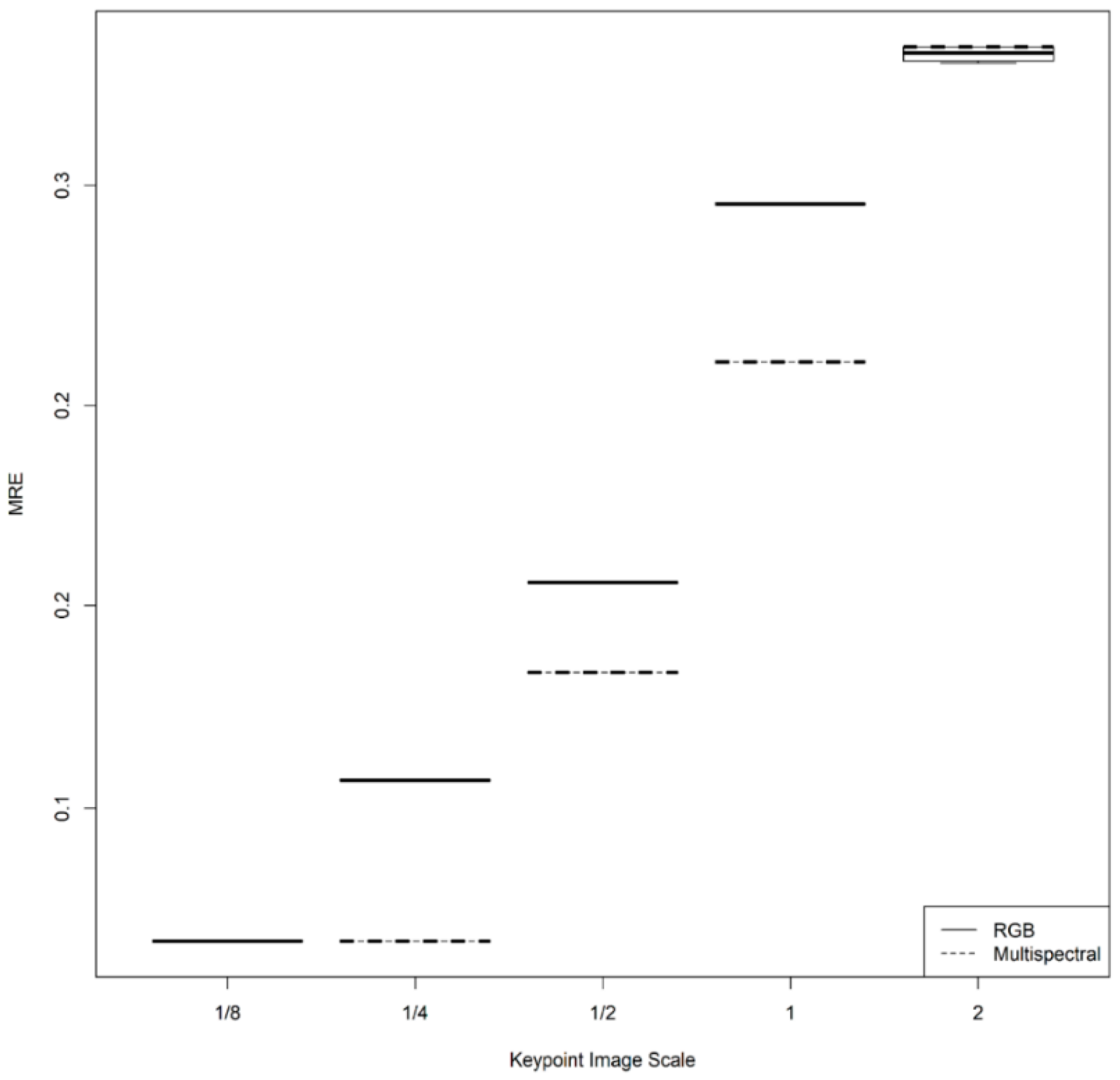
In the next phase of intermediary product generation, the bundle block adjustment (BBA) process, RGB imagery results in more 3D points for the BBA (3DKP) than multispectral imagery in 1/4 through to full (1) keypoint scales. The differences are, on average, three orders of magnitude higher for RGB imagery (Figure 8). The difference between processing at full (1) vs. two times (2) the keypoint scale results in significantly higher 3D points for multispectral than RGB imagery, with RGB presenting some variability in the trials at two times (2) the keypoint scale. Finally, one of the last intermediary products we examined, the mean reprojection error (MRE), reveals that RGB has higher MRE than multispectral imagery (except for 1/8, where multispectral processing failed) and that MREs are nearly identical for two times (2) the keypoint scale, on the order of 0.3–0.4 (Figure 9).

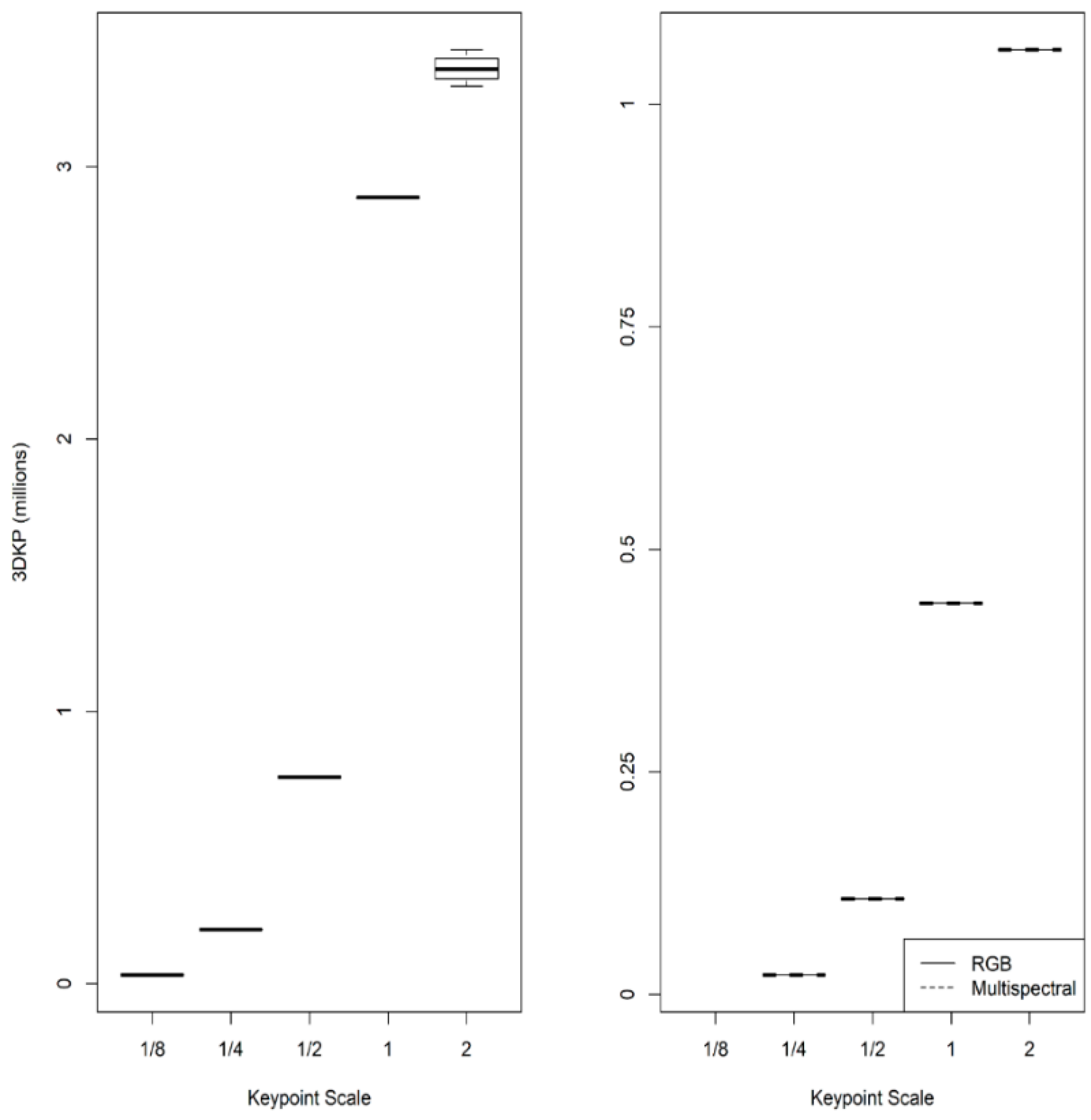
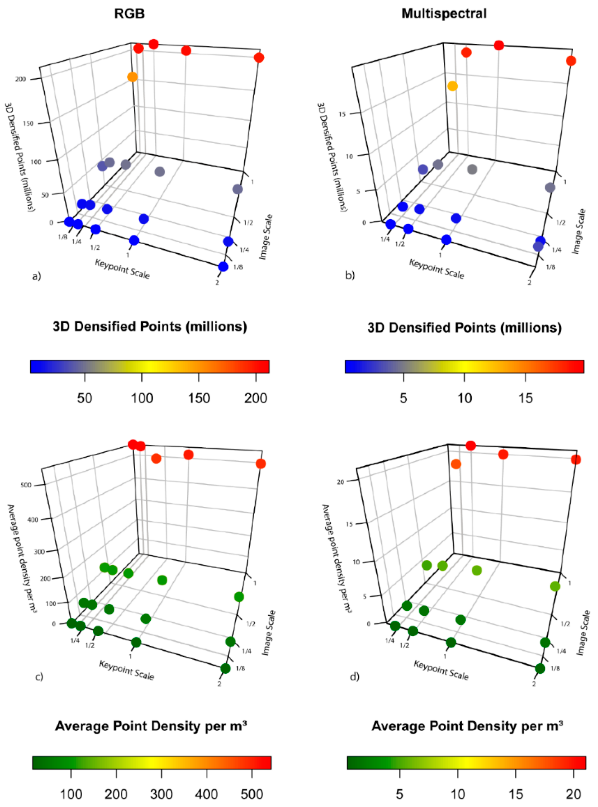
When moving towards the point cloud densification stages of processing (refer back to Figure 1), we analyzed the effects on the number of 3D densified points (3DDP) generated as keypoint scale and image scale were varied. For imagery collected with an RGB camera, we observed increasing 3DDP with increasing image scale and more variation in 3DDP as the keypoint scale is increased (Figure 10a). For multispectral trials, variation in the number of 3DDP again increased with increasing keypoint scale and generally, more points were produced as the image scale increased. For multispectral trials, 3DDP was highest at full (1) keypoint scale and full (1) image scale, compared to 1/2 keypoint scale and full image scale for RGB (Figure 10a,b). The average point density for RGB increased with increasing image scale and exhibited slight variation in the number of dense points at full (1) image scale (Figure 10c). The average point density for multispectral also increased with increasing image scale and had more variation between different keypoint scales as the image scale increased (Figure 10d). The highest average point densities for RGB imagery occurred between 1/8 to 1/4 keypoint scales and full image scale, whereas for multispectral imagery, the highest average point density occurred at 1/2 keypoint scale (Figure 10c,d). The imagery processed at full (1) image scale produced 3DDP and point density results that were significantly different from 3DDP and point density results when imagery was processed at lower image scales in both RGB and multispectral imagery (

Table 6. Statistical differences between three-dimensional densified points (3DDP) and average point density (PtDens) at one (1) image scale compared to all other keypoints—for image scale combinations, see Figure 10. Processing trials at one (1) image scale differed significantly from all other trials for both 3DDP and PtDens.

	RGB			Multispectral
	t-Stat	df	p-Value	t-Stat	df	p-Value
3DDP	15.05	60.93	0.00	9.42	3.78	0.00
PtDens	32.12	11.70	0.00	19.13	9.13	0.00

). Based on these results, we conclude that RGB data is capable of producing better 3D products at lower processing parameter values, whereas multispectral requires higher (thus more computationally intensive) processing parameter values to obtain similar point cloud densities.

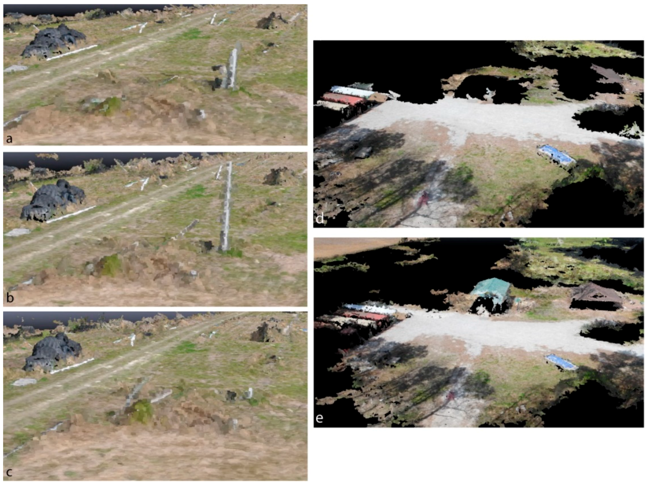
To visualize the results of these processing trials for 3D object reconstruction, we examine objects reconstructed from imagery in Area A (Figure 2) again, but this time, consider how varying image scale for point cloud densification affects DSM generation (Figure 11). The red roof and black roof buildings are not visible for RGB because this is shown as a constant 1/2 keypoint scale where they were not interpolated accurately (Figure 7). We observe that as image scale for point cloud densification increases, the building edges become more distinct, sharper, and less blurry. Small features, such as the rows of tires in the lower right corner (refer to orthomosaic in Figure 7D), become more distinct. Multispectral imagery was able to interpret the presence of the building not detected by RGB, though overall, the object definition quality is not as good for multispectral compared to RGB if we are comparing results generated using the same settings. For example, reconstruction 11A and 11E use the same settings and though more structures were detected in 11E (multispectral) than 11A (RGB), the DSM quality is much poorer (Figure 11). However, it is possible to obtain good-quality DSMs from multispectral imagery if higher image scale settings are used in processing. For example, reconstruction 11A and 11H were processed using different image scales (1/8 and full, respectively) but resulted in similar-quality DSMs in terms of building sharpness, with the obvious advantage of multispectral being that it was accurately able to resolve buildings that RGB did not. These findings have important implications for users whose primary objective is using multispectral data for vegetation analyses, for instance, because it means they can process the imagery at higher settings and obtain reliable and comparable 3D surfaces as they would otherwise using the higher resolution RGB cameras that are typically thought to offer an advantage for 3D scene reconstructions.

Using constant, full (1) image scale for point cloud densification and varying the keypoint scale (see Figure 12), we created visual (RGB) representations of features in the densified point cloud that stand out in an image, in this case, a more linear feature (tall Pine tree trunk, Figure 12a–c) and a polygonal feature (a shed on the property we surveyed, Figure 12d,e). For the two types of objects of interest, linear and polygonal, the best rendering in 3D space appears inconsistent between the two, with linear features detected more accurately at 1/2 keypoint scale and at two (2) keypoint scale for areal features (Figure 12d,e).

Previous UAS work over a forested plot at different flight heights, using the same RGB (SenseFly S.O.D.A. sensor) and multispectral (the Parrot Sequoia sensor) cameras we used in this study, compared image processing in both Pix4D and AgiSoft Photoscan [7]. However, they only used 1/2 for keypoint scale and 1/4 for image scale for point cloud densification in Pix4D to reduce scene complexity while extracting visual information and to further simplify raw image geometry while computing 3D coordinates [7]. They noted that those two parameter selections would lead to faster processing in complex landscapes but could influence accuracy, yet the degree and magnitude of changes in accuracies were not investigated as we did in this study [7]. Gross and Heumann [5] used full (1) keypoint scale and 1/4 for image scale for point cloud densification, noting, however, that most similar previous studies [8,9] only assessed geometric accuracy of different software processing systems and were generally concerned with assessing final product quality, with little quantitative attention paid to intermediary products as we did in this work. Finally, work by Sona et al. [8] compared outputs from multiple imagery processing software packages but did not state explicitly what parameter values were used or why these were chosen, noting, however, that when comparing Pix4D and AgiSoft, for instance, that Pix4D identified fewer matched points overall but was able to detect more visible points in more images. Even though we did not compare multiple processing software packages, our work provides a set of guidelines for choosing the appropriate and case-specific initial and intermediary processing parameters for RGB and multispectral imagery to ensure the most appropriate final products are generated.

5. Conclusions

In this paper, we explored the effects of varying keypoint image scale and image scale selection parameters on DSM/DTM and orthomosaic generation in a structure-from-motion workflow implemented in Pix4D Mapper Pro for both RGB and multispectral imagery. We showed that, despite generally lower GSD, multispectral data performed better overall for detecting edges, small features, and minute changes in surface elevations in final products resulting from photogrammetric processing. In both RGB and multispectral imagery, sharp edges and small features can become altogether lost depending on processing parameters for 3D object generation. By iterating through 40 processing sets of parameters, varying one parameter at a time, we conclude that maximizing for the highest intermediate parameters may not always translate into effective final products and that if users plan to use the highest processing parameters, the most important measure to be taken to ensure quality end products is to increase initial flight coverage in advance. Finally, we showed that, even though multispectral imagery has lower GSD compared to RGB data, one could obtain a similar-quality DSM from multispectral data as you could RGB if higher settings are used in processing. This fact has important implications for users whose primary objective is using multispectral data for vegetation analyses, for instance, because it means they can process the imagery at higher settings and obtain reliable and comparable 3D surfaces as they would otherwise using higher resolution RGB cameras, which are typically thought to offer an advantage for 3D scene and structural reconstructions.

References

1. Salami, E.; Barrado, C.; Pastor, E. UAV Flight Experiments Applied to the Remote Sensing of Vegetated Areas. Remote Sens. 2014, 6, 11051–11081. [Google Scholar] [CrossRef] [Green Version]
2. Zhou, G.Q.; Ambrosia, V.; Gasiewski, A.J.; Bland, G. Foreword to the Special Issue on Unmanned Airborne Vehicle (UAV) Sensing Systems for Earth Observations. IEEE Trans. Geosci. Remote Sens. 2009, 47, 687–689. [Google Scholar] [CrossRef]
3. Wallace, L.; Lucieer, A.; Watson, C.; Turner, D. Development of a UAV-LiDAR System with Application to Forest Inventory. Remote Sens. 2012, 4, 1519–1543. [Google Scholar] [CrossRef] [Green Version]
4. Anderson, K.; Gaston, K.J. Lightweight unmanned aerial vehicles will revolutionize spatial ecology. Front. Ecol. Environ. 2013, 11, 138–146. [Google Scholar] [CrossRef] [Green Version]
5. Gross, J.W.; Heumann, B.W. A statistical examination of image stitching software packages or use with unmanned aerial systems. Photogramm. Eng. Remote Sens. 2016, 82, 419–425. [Google Scholar] [CrossRef]
6. Pix4D. Pix4Dmapper Pro; [Computer Software]; Pix4D: Prilly, Switzerland, 2019. [Google Scholar]
7. Fraiser, B.T.; Congalton, R.G. Issues in unmanned aerial systems (UAS) data collection of complex forest environments. Remote Sens. 2018, 10, 908. [Google Scholar] [CrossRef]
8. Sona, G.; Pinto, L.; Pagliari, D.; Passoni, D.; Gini, R. Experimental analysis of different software packages for orientation and digital surface modeling from UAV images. Earth Sci. Inform. 2014, 7, 97–107. [Google Scholar] [CrossRef]
9. Turner, D.; Lucieer, A.; Wallace, L. Direct georeferencing of ultrahigh-resolution UAV imagery. IEEE Trans. Geosci. Remote Sens. 2014, 52, 2738–2745. [Google Scholar] [CrossRef]
10. Westoby, M.J.; Brasington, J.; Glasser, N.F.; Hambrey, M.J.; Reynolds, J.M. Structure-from-motion photogrammetry: A low-cost, effective tool for geoscience applications. Geomorphology 2012, 179, 300–314. [Google Scholar] [CrossRef]
11. Lowe, D.G. Distinctive image features from scale-invariant keypoints. Int. J. Comput. Vis. 2004, 60, 91–110. [Google Scholar] [CrossRef]
12. Bay, H.; Tuytelaars, T.; Van Gool, L. SURF: Speeded up robust features. In Computer Vision-ECCV 2006; Springer: Berlin/Heidelberg, Germany, 2006; pp. 404–417. [Google Scholar]
13. Leutenegger, S.; Chli, M.; Siegwart, R.Y. BRISK: Binary robust invariant scalable keypoints. In Proceedings of the IEEE International Conference on Computer Vision, ICCV 2011, Barcelona, Spain, 6–13 November 2011; pp. 2548–2555. [Google Scholar]
14. SenseFly. eMotion; [Computer Software]; senseFly: Cheseaux-sur-lausanne, Switzerland, 2019. [Google Scholar]
15. R Core Team. R; [Computer Software]; R Core Team: Vienna, Austria, 2017. [Google Scholar]
16. Wei, T.; Simko, V.; Levy, M.; Xie, Y.; Jin, Y.; Zemla, J. Corrplot: Visualization of a Correlation Matrix. R Package Version 0.84. 2016. Available online: https://cran.r-project.org/web/packages/irr/index.html (accessed on 29 June 2019).
17. Soetaert, K. Plot3d: Plotting Multi-Dimensional Data. R Package Version 1.1.1. 2017. Available online: https://rdrr.io/cran/plot3D/ (accessed on 29 June 2019).
18. ESRI. ArcGIS; [Computer Software]; ESRI: Redlands, CA, USA, 2017. [Google Scholar]
19. Friendly, M. Corrgrams: Exploratory displays for correlation matrices. Am. Stat. 2002, 56, 316–324. [Google Scholar] [CrossRef]
Figure 1. Key photogrammetric processing steps in the structure-from-motion workflows for RGB and multispectral imagery (as implemented in Pix4Dmapper Pro).
Drones 03 00063 g001
Figure 2. Study Area. The orthomosaic shown was generated from the iteration using full (1) keypoint scale and half (1/2) image scale for point cloud densification. Colored lines represent the digitized boundaries from other processing iterations at half (1/2) image scale for point cloud densification to show the variation in amount of area covered in the final orthomosaics based on percent calibrated images.
Drones 03 00063 g002
Figure 3. Correlation plot for RGB and multispectral processing result metrics (see Table 3 for a description of metrics). Only results that were statistically significant (p > 0.05) are displayed. The bottom-right corner of the diagram displays the actual correlation value, while the top right corner is a visual representation of the sign and magnitude of the correlation value. The color scale uses blue to represent positive correlation values and red to represent negative correlation values.
Drones 03 00063 g003
Figure 4. Percent of images calibrated with varying keypoint image scale for RGB and multispectral imagery. Refer to Figure 2 to see how percent image calibration affects the areal coverage in the final orthomosaics. The percent of images calibrated differed significantly between RGB and multispectral processing trials (df = 24.97, p = 0.03). A single line indicated there was no variation between image scales at a given keypoint. A box-and-whisker diagram is displayed, where variation exists between different image scales at a given keypoint scale, where the box displays the interquartile range, the line through the middle of the box represents the median, the upper whisker represents the maximum value, and the lower whisker represents the minimum value. All multispectral processing trials at 1/8 keypoint scale failed to process, thus there are no results displayed.
Drones 03 00063 g004
Figure 5. Median number of matches with varying keypoint image scale for RGB and multispectral imagery. The median number of matches per image differed significantly between RGB and multispectral processing trials (df = 19.54, p = 0.00). As in Figure 4, a single line indicates no variation in results across image scales and a box-and-whisker plot is shown if variation exists. All multispectral processing trials at 1/8 keypoint scale failed to process, thus there are no results displayed.
Drones 03 00063 g005
Figure 6. Number of 2-D keypoints observed for bundle block adjustment with varying keypoint image scale for RGB and multispectral imagery. The number of 2-D keypoints observed for bundle block adjustment did not differ significantly between RGB and multispectral processing trials (df = 21.70, p = 0.59). As in previous figures, a single line indicates no variation in results across image scales and a box-and-whisker plot is shown if variation exists. All multispectral processing trials at 1/8 keypoint scale failed to process, thus there are no results displayed.
Drones 03 00063 g006
Figure 7. Effect of varying keypoint scale at full (1) image scale for point cloud densification for RGB (AF) and multispectral (GJ) imagery. Keypoint scales: (A) (1/8), (B,G) (1/4), (C,H) (1/2), (E,I) (1), (F,J) (2). D shows the corresponding scene in the orthomosaic (inset refers to Area A in study area Figure 2).
Drones 03 00063 g007
Figure 8. Number of 3D points for bundle block adjustment (3DKP) with varying keypoint scale for RGB and multispectral imagery. The number of 3D points for bundle block adjustment differed significantly between RGB and multispectral processing trials (df = 22.99, p = 0.01). A single line indicates no variation in results across keypoint scales and a box-and-whisker plot is shown if variation exists. All multispectral processing trials at 1/8 keypoint scale failed to process, thus there are no results displayed.
Drones 03 00063 g008
Figure 9. Mean reprojection error with varying keypoint scale for RGB and multispectral imagery. Mean reprojection error did not differ significantly between RGB and multispectral processing trials (df = 32.08, p = 0.08). A single line indicates no variation in results across keypoint scales and a box-and-whisker plot is shown if variation exists. All multispectral processing trials at 1/8 keypoint scale failed to process, thus there are no results displayed.
Drones 03 00063 g009
Figure 10. Number of three-dimensional densified points (3DDP) and average point density per cubic meter (PtDens) for RGB (a,b) and multispectral (c,d) imagery. There were significant differences between RGB and multispectral imagery both 3DDP and PtDens (df = 19.07, p = 0.00; and df = 19.07, p = 0.00, respectively). We also tested to see if processing trials at one (1) image scale were significantly different than at all other keypoints scale—image scale combinations for both 3DDP and PtDens see Table 6.
Drones 03 00063 g010
Figure 11. Effect of varying image scale (1/8 for (A,E), ¼ for (B,F), ½ for (C,G), and 1 for (D,H)) for point cloud densification with a constant keypoint image scale of half (1/2) in Area A (Figure 2). Half image scale is the Pix4D default and also resulted in the highest calibrated image percent for RGB imagery trials in this study (see Figure 4).
Drones 03 00063 g011
Figure 12. Feature detection performance visualized in the point cloud using full image scale for point cloud densification and keypoint scale as follows: (ac) are 1/8, 1/2, and 2; (d,e) are 1/8 and 2.
Drones 03 00063 g012