Positional Precision Analysis of Orthomosaics Derived from Drone Captured Aerial Imagery

Abstract

The advancement of drones has revolutionized the production of aerial imagery. Using a drone with its associated flight control and image processing applications, a high resolution orthorectified mosaic from multiple individual aerial images can be produced within just a few hours. However, the positional precision and accuracy of any orthomosaic produced should not be overlooked. In this project, we flew a DJI Phantom drone once a month over a seven-month period over Oak Grove Cemetery in Nacogdoches, Texas, USA resulting in seven orthomosaics of the same location. We identified 30 ground control points (GCPs) based on permanent features in the cemetery and recorded the geographic coordinates of each GCP on each of the seven orthomosaics. Analyzing the cluster of each GCP containing seven coincident positions depicts the positional precision of the orthomosaics. Our analysis is an attempt to answer the fundamental question, “Are we obtaining the same geographic coordinates for the same feature found on every aerial image mosaic captured by a drone over time?” The results showed that the positional precision was higher at the center of the orthomosaic compared to the edge areas. In addition, the positional precision was lower parallel to the direction of the drone flight.

1. Introduction

Aerial photography began to be used on a routine basis in the 1920s with the advent of modern film and aircraft [1]. Current use of unmanned aerial systems (UAS), commonly referred to as drones, has combined aerial photography and remote sensing to expand into successful businesses incorporating both individual users and governmental agencies to map the Earth surface on a repetitive basis [2]. Until digital cameras became available, creating a mosaic of aerial photograph required considerable work, time, energy, and expense, even after computers became widely available. In analog aerial photography, after each film roll was exposed, it had to be processed, printed, scanned, and georeferenced. Then the stitching process applies algorithms to minimize image distortion in order to produce an orthorectified aerial photomosaic [3].

The United States Geological Survey (USGS) produces a series of digital aerial photographs of the country known as a DOQ (digital orthophoto quadrangle), with each covering an area of 7.5-minutes of longitude by 7.5-minutes of latitude. DOQ has since become the general term when referring to an orthorectified aerial photograph in digital format. When a DOQ is split to four quadrats for file management purpose, it is known as a DOQQ (digital orthophoto quarter quadrangle), a term widely used in the geographic information systems (GIS) community.

While processing traditional aerial photographs was time consuming, taking those photos from an airplane was equally complicated. It involved developing a flight plan, calculating optimum flying altitude, determining optimum overlap and endlap relative to along and adjacent to any flight paths, maintaining an aerial plane with a pilot and a photographer, a ground crew for setting ground control points, etc.

This workflow has been simplified when UAS became commonplace within the remote sensing community. Coupled with the flight control software, a drone can be flown to acquire aerial imagery within a programed location with the set height, flight paths, overlaps, and camera settings [2]. With the drone’s onboard global positioning system (GPS), the positional accuracy of the imagery equals the GPS receiver. When the drone image files are loaded into a digital image processing program, they are stitched together to produce an orthomosaic, similar to a traditional DOQQ. This process for the drone imagery can be completed on a desktop computer in a timely and cost effective manner [4]. The completed orthomosaic images feature detailed ground surface with high spatial resolution. These methods decrease cost, reduce risk, and produce high accuracy potential [2,5].

While traditional aerial photography from a manned airplane continues to serve projects of large areas, especially when acquiring aerial photography at a small scale, drone acquired imagery is suitable for smaller and inaccessible areas with the drone user controlling the spatial, spectral, radiometric, and temporal resolution of the product [6,7,8,9]. With limited capital investment, the process from setting up a drone flight to the output of a rectified orthomosaic image for a specific area can be achieved within hours [5,10], providing timely cost-effective monitoring of the forest environment [11,12]. Advantages of a UAS for mapping of small areas include high spatial resolution, the ability to complete time series imagery, potentials for 3D imagery to produce both orthomosaics and 3D models, and the integration into community-based forest monitoring (CBFM) or habitat monitoring [13].

Nogueira et al. [5] utilized Pix4D Mapper Pro to process images from a DJI Phantom 4 Pro drone for mapping accuracy of a 15-hectare site with ground control points (GCPs). Pix4D Mapper is a software application that allows the user to process images captured by an aerial vehicle and generate georeferenced models for GIS output. Their findings indicated that low features were well defined but tops of trees were not. The central region of the image provided better results than the edges. Digital surface models and planimetry error vectors for the orthomosaic with and without ground control points were displayed. Also, GCPs with known coordinates increased the accuracy of UAS flights [14,15]. Lima et al. [16] demonstrated the accuracy of the DJI Phantom 4 Pro UAS for three-dimensional coordinates using Pix4D Mapper Pro software with 15 ground control points and 47 checkpoints, concluding that the coordinates and attitude angles of the UAS camera can be measured. Tomastik et al. [17] found that with forest sites of one hectare or less, GCP quantity was not as important as the configuration but additional GCP increased accuracy. For best accuracy and quality control with UAS, GCP are needed [5,14,18,19]. With all the advantages of using a drone for aerial photography, a question still needs to be asked. What is the precision and accuracy of a drone derived aerial orthomosaic? To explore the quality of drone acquired imagery in producing orthomosaics, we conducted a series of drone flights over the same area and produced a digital aerial orthomosaic for each flight. The goal was to access its geographic precision of location to ascertain if each orthomosaic resulted in the same geographic coordinates for a ground feature identified on the digital orthomosaic.

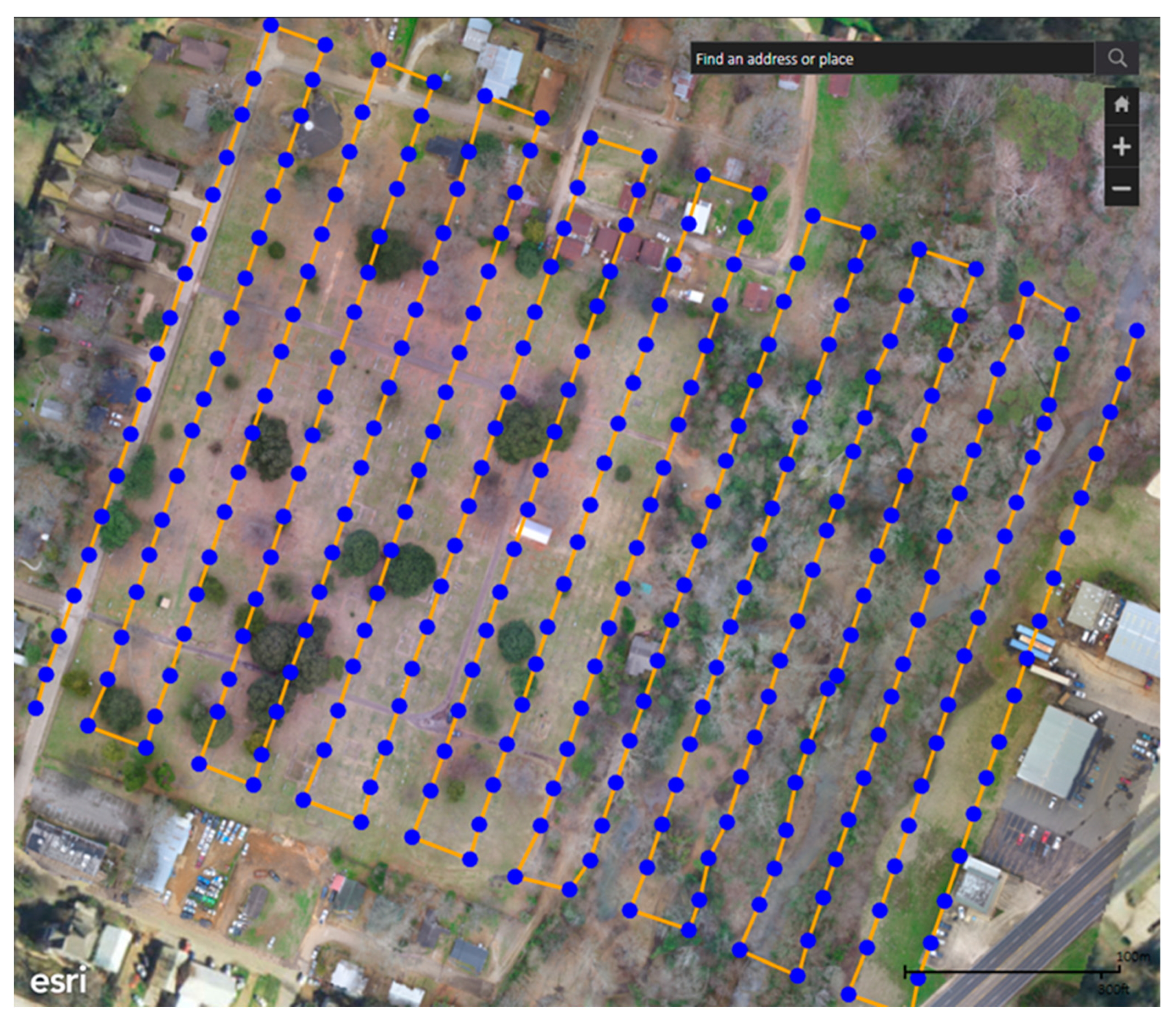
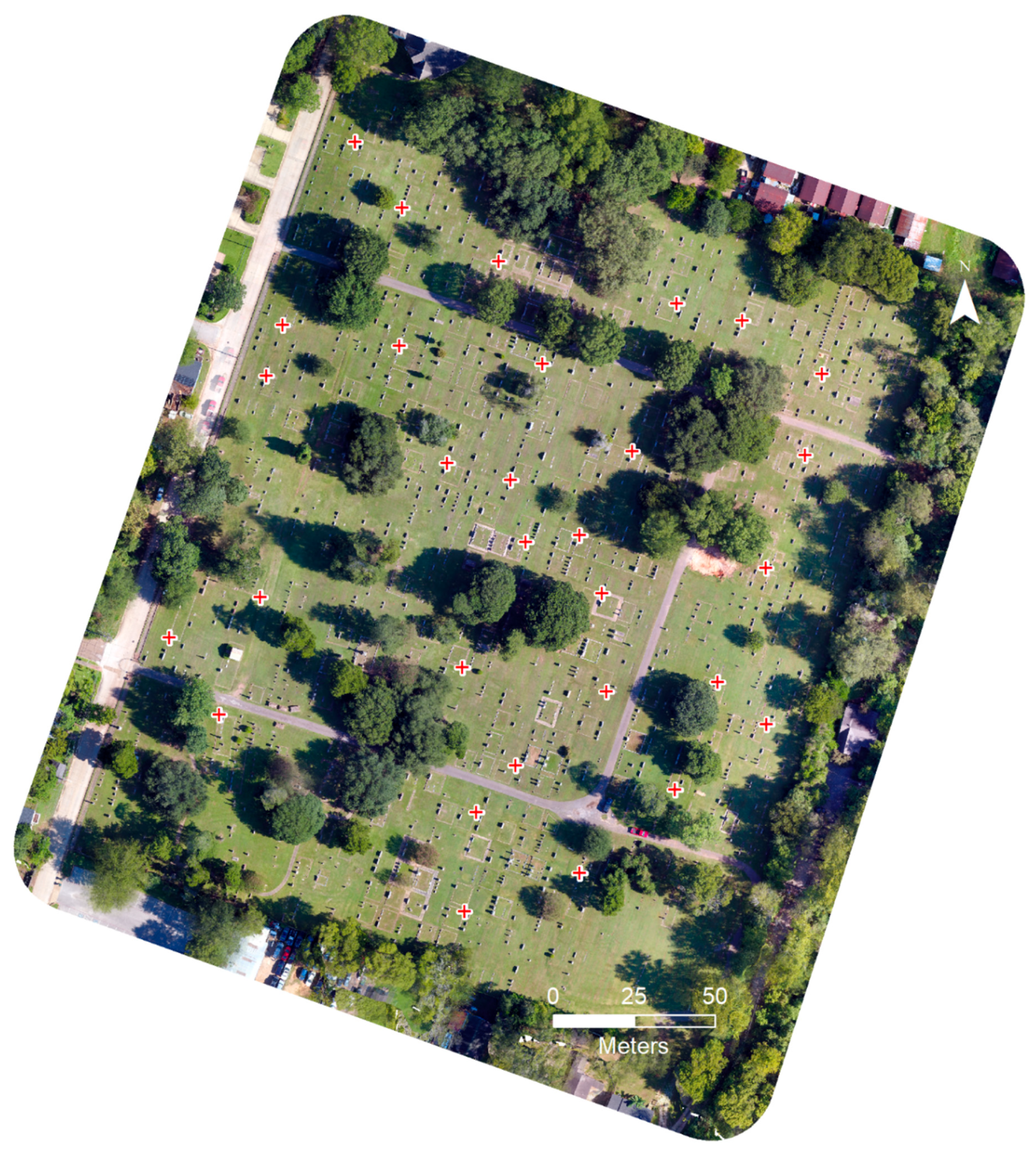
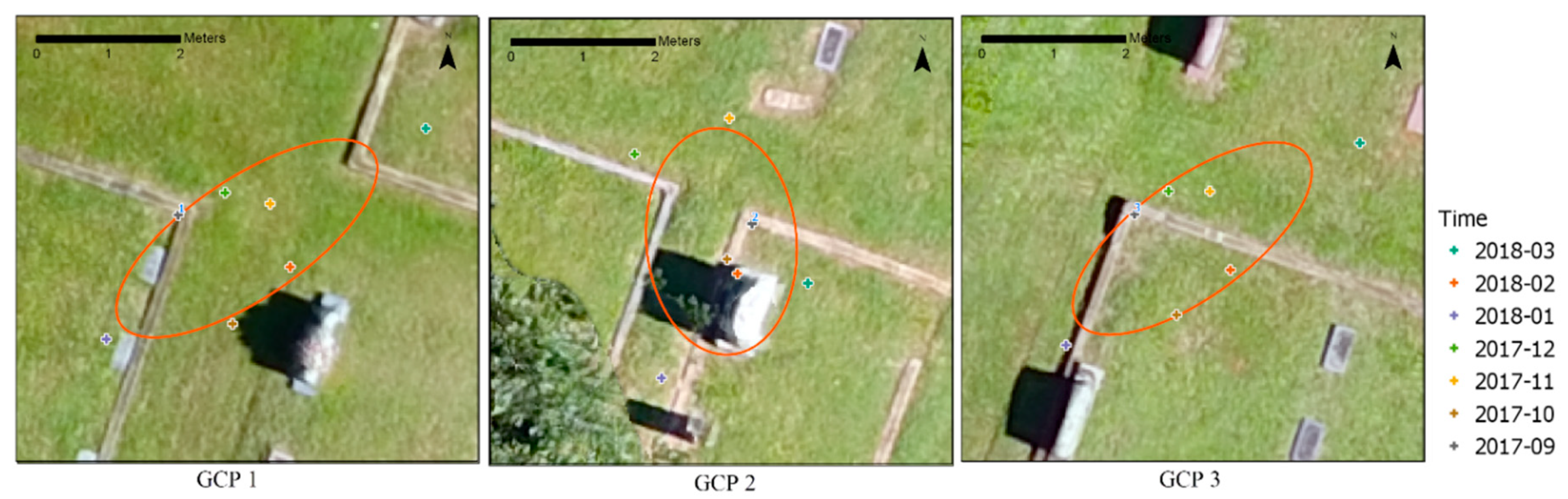
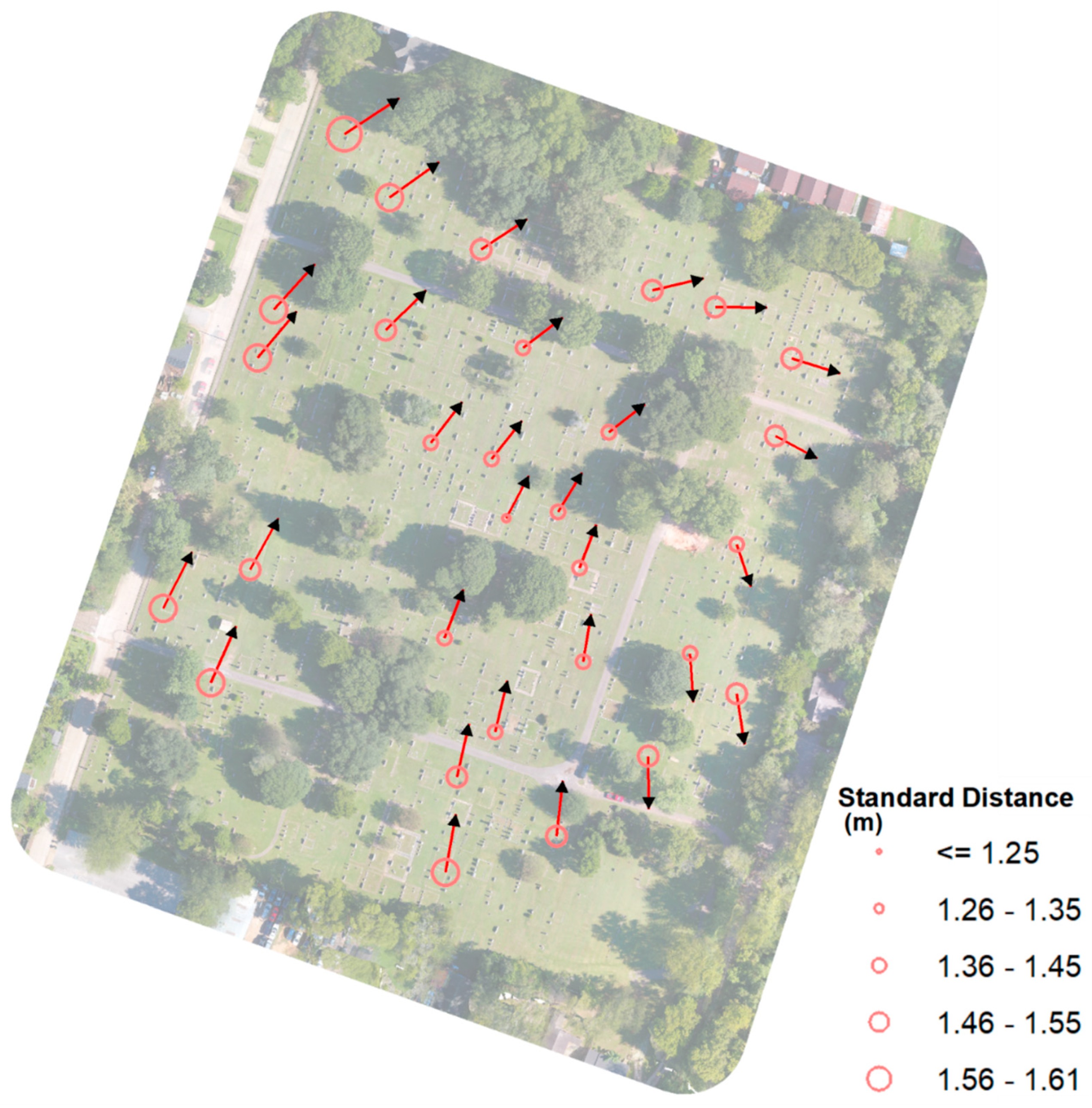
2. Materials and Methods

The study area chosen to assess the positional precision of orthomosaics derived from drone acquired imagery was the historic Oak Grove Cemetery located next to downtown Nacogdoches in east Texas, USA. Oak Grove Cemetery, consisting of 5.2 ha (12.7 ac) of cemetery plots with intermingled pine and hardwood trees, was chosen due to its permanent features that are readily identifiable within digital imagery and suitable for a precision assessment on positions identified on repeated aerial imagery. A DJI Phantom 3 or 4 drone was flown over the study area monthly from September 2017 to March 2018, depending on which DJI model was available for each scheduled flight. The comparison on specifications between the two drones is shown in

Table 1. Comparison of the two drone models used.

Specifications	DJI Phantom 3 Advanced	DJI Phantom 4 Professional
Weight	1280 g	1388 g
Diagonal size	350 mm	350 mm
Max speed	57.6 km/h	72.0 km/h
Max serve celling MSL	6000 m	6000 m
Max flight time	23 min	30 min
GNSS	GPS/GLONASS	GPS/GLONASS
Camera lens	FOV 94°, 20 mm, f/2.8	FOV 84°, 24 mm, f/2.8-f11
Image sensor	1/2.3” CMOS, 12.4M pixels	1” CMOS, 20.0M pixels
Hover Accuracy
Vertical:	±0.1 m (with Vision Positioning)	±0.1 m (with Vision Positioning)
	±0.5 m (with GPS Positioning)	±0.5 m (with GPS Positioning)
Horizontal:	±0.3 m (with Vision Positioning)	±0.3 m (with Vision Positioning)
	±1.5 m (with GPS Positioning	±1.5 m (with GPS Positioning

. Both had a similar physical size and camera lens, while the Phantom 4 had a larger image sensor. However, they resulted in spatial resolutions of orthomosaic that were within a comparable range (

Table 2. Summary of drone flight missions and orthomosaics produced.

Date of Flight	Number of Photos Used for the Mosaic	Spatial Resolution of the Mosaic (cm)	Drone Model Used
9/7/2017	378	2.73	Phantom 4
10/17/2017	288	2.95	Phantom 3
11/13/2017	288	2.95	Phantom 3
12/14/2017	286	2.89	Phantom 3
1/15/2018	230	2.78	Phantom 3
2/15/2018	306	2.89	Phantom 3
3/6/2018	168	2.57	Phantom 4

). In addition, both drone models had the same hover accuracy that is deemed to be appropriate for comparison on positional precision analysis. Each drone flight was conducted as a grid mission using the Pix4DCapture app installed on an iPad, with the flight height set at 67 m (220 ft), front overlap set at 80%, side overlap set at 60%, and the angle of the camera set at 80 degrees. Each drone mission took an average flight time of 17 minutes, resulting in an average of 306 photos covering a total area of 11.7 ha (28.9 ac). Each drone flight was planned to fly outside the boundaries of the cemetery to ensure any resulting orthomosaic produced from each drone flight would completely contain the physical boundaries of the entire cemetery (Figure 1). Weather conditions at the time of each flight were observed based on the weather station located at the East Texas Regional Airport (

Table 3. Weather conditions at the time of each flight.

Date	9/7 2017	10/17 2017	11/13 2017	12/14 2017	1/15 2018	2/15 2018	3/6 2018
Time	10:00	10:30	10:30	12:00	14:15	12:30	9:30
Temperature (C)	26.1	24.4	17.8	13.3	6.1	22.8	20.0
Dew Point (C)	11.1	3.9	15.0	1.7	5.6	18.3	−6.1
Humidity (%)	39	26	83	45	97	76	17
Wind Direction	Variable	ENE	NE	NNW	N	S	NNW
Wind Speed (km/h)	8.1	11.3	9.7	4.8	16.1	11.3	22.5
Wind Gust (km/h)	0	0	0	0	0	0	35.4
Pressure (mm Hg)	757	757	759	752	762	752	752
Weather Condition	Fair	Fair	Cloudy	Fair	Cloudy	Mostly Cloudy	Fair

). They were considered fair for flying a drone for aerial photography.

Upon the completion of each drone mission, images acquired by the drone were imported into Drone2Map to create an orthomosaic. Default settings were used in Drone2Map for creating each month’s 2D orthomosaic, with output image resolution set automatically that resulted in the cell size of each orthomosaic ranging from 2.78–2.95 cm for the Phantom 3 and 2.57–2.73 cm for the Phantom 4 DJI drones, respectfully. Each output mosaicked image was referenced to WGS 1984 UTM Zone 15N. A total of seven orthomosaics of the Oak Grove Cemetery were produced.

In order to assess the precision of positions, 30 ground control points were selected throughout the cemetery based on the 7 September 2017 orthomosaic. Each GCP was selected on a distinguishable corner of a family plot in the cemetery. Family plot corners were chosen as they were easily distinguishable visually both in the orthomosaics and easily identifiable on the ground. The UTM coordinates of each GCP were acquired by creating a point feature through on-screen digitization with an orthomosaic as the reference image. This process was repeated seven times on each of the seven orthomosaics produced. The outcome was a group of seven spatial point features for each GCP, where all of the seven represent the same feature on the ground (Figure 2).

To analyze the geographic distribution of the seven positions of each GCP, the mean center of each cluster (Equation (1)) was first calculated. The mean center is plotted based on the mean x coordinate and mean y coordinate of all seven positions and represents the geographic center of each cluster. Then, the standard distance for summary circle (Equation (2)) was calculated that depicts the dispersion of the positions around the same feature. A lower standard distance translates to higher precision, where the seven positions are closer to each other. Finally, when directional effect of each cluster is considered, the standard deviational ellipse (Equation (3)) was calculated. It shows the direction where the precision is diluted most than others. All geographic distribution data were plotted on an orthomosaic and analyzed visually to identify spatial patterns in each GCP’s spatial distribution over the seven orthomosaics produced (see Supplementary Materials).

$$\overline{S}=\left({\mu }_x,{\mu }_y\right)=\left(\frac{{{\displaystyle \sum }}_{i=1}^n{x}_i}{n},\frac{{{\displaystyle \sum }}_{i=1}^n{y}_i}{n}\right)$$

(1)

$$d=\sqrt{\frac{{{\displaystyle \sum }}_{i=1}^n{\left(x_i-{\mu }_x\right)}^2+{\left(y_i-{\mu }_y\right)}^2}{n}}$$

(2)

$$d_x=\sqrt{\frac{{{\displaystyle \sum }}_{i=1}^n{\left(x_i-{\mu }_x\right)}^2}{n}} d_y=\sqrt{\frac{{{\displaystyle \sum }}_{i=1}^n{\left(y_i-{\mu }_y\right)}^2}{n}}$$

(3)

3. Results

For each GCP, the geographic coordinates were attained seven times based on the seven orthomosaics, one for each month. Figure 3 depicts the seven positions of the same GCP when plotted on the September 2017 orthomosaic, where the GCP no. 1 to 3 were presented and a standard deviational ellipse indicated the dilution of precision for the position cluster of each GCP. Based on UTM Zone 15N, WGS 84, the x and y coordinates of mean center, standard distance of summary circle, azimuth of deviational ellipse rotation, major and minor semi-axis of ellipse, and area of the ellipse for each position cluster of representing all GCP’s are summarized in Appendix A,

Table A1. Position cluster statistics for each ground control point (GCP) based on seven orthomosaics.

GCP ID	X Coordinate of Mean Center (m)	Y Coordinate of Mean Center (m)	Standard Distance of Summary Circle (m)	Azimuth of Ellipse Rotation (degree)	Major Semi-axis of Ellipse (m)	Minor Semi-axis of Ellipse (m)	Area of Deviational Ellipse (sq m)
1	343,565.68	3,497,810.96	1.61	55.87	2.12	0.83	5.50
2	343,676.42	3,497,644.76	1.34	175.20	1.57	1.04	5.16
3	343,580.11	3,497,790.65	1.51	53.83	1.97	0.81	5.03
4	343,609.61	3,497,774.07	1.40	55.51	1.76	0.92	5.07
5	343,664.44	3,497,760.95	1.42	75.93	1.68	1.11	5.84
6	343,684.57	3,497,755.69	1.43	89.75	1.65	1.17	6.08
7	343,709.08	3,497,739.19	1.44	106.33	1.63	1.22	6.24
8	343,543.03	3,497,754.76	1.49	41.41	1.98	0.74	4.57
9	343,578.99	3,497,748.25	1.40	44.47	1.82	0.78	4.48
10	343,622.92	3,497,742.58	1.33	52.03	1.60	0.99	4.99
11	343,650.46	3,497,715.59	1.31	51.15	1.47	1.13	5.25
12	343,703.78	3,497,714.32	1.40	117.54	1.53	1.26	6.05
13	343,691.44	3,497,679.65	1.33	160.45	1.43	1.21	5.45
14	343,612.96	3,497,706.88	1.29	37.25	1.57	0.93	4.57
15	343,642.22	3,497,641.95	1.29	8.35	1.55	0.95	4.63
16	343,601.89	3,497,605.10	1.37	11.42	1.75	0.83	4.60
17	343,537.89	3,497,739.31	1.48	39.11	1.96	0.71	4.35
18	343,593.37	3,497,712.18	1.31	36.76	1.65	0.82	4.27
19	343,617.63	3,497,687.93	1.25	26.93	1.54	0.89	4.29
20	343,634.19	3,497,689.96	1.28	30.23	1.48	1.04	4.82
21	343,641.02	3,497,672.01	1.27	20.54	1.49	1.00	4.69
22	343,691.46	3,497,631.79	1.41	170.69	1.65	1.12	5.79
23	343,663.07	3,497,611.75	1.38	178.48	1.69	0.98	5.23
24	343,614.02	3,497,619.44	1.34	12.66	1.70	0.86	4.56
25	343,597.85	3,497,649.51	1.31	19.77	1.67	0.78	4.10
26	343,535.58	3,497,671.47	1.43	27.69	1.88	0.75	4.43
27	343,507.68	3,497,659.14	1.54	25.95	2.03	0.81	5.15
28	343,522.87	3,497,635.29	1.51	23.01	1.99	0.80	4.98
29	343,598.13	3,497,574.59	1.48	9.18	1.89	0.90	5.34
30	343,633.66	3,497,586.16	1.42	5.81	1.79	0.90	5.05

. The standard distances ranged from 1.25 m to 1.61 m, with lower values indicating higher precision of a cluster of seven positions for an individual GCP.

In Figure 4, the rotation of the summary ellipses showed a clockwise pattern with azimuths ranging from 6 to 178 degrees. Most of the summary ellipses (80%) have their major axis oriented along the direction pointing northeast and southwest (Figure 5). Those GCP clusters oriented southeast and northwest (20%) were found along the east side boundary of the study area. On average, the rotation has a mean azimuth of 60 degrees and a mean major semi-axis of 1.72 m.

4. Discussion

The seven flights programmed with Pix4DCapture each resulted images that were processed with Drone2Map. It created a series of georectified images that could be compared month to month based on set GCPs. The resulting images indicated a dilution of positional precision in the data over time with primarily a northeast direction. When presented in a map context (Figure 4), the positions of a GCP are more clustered at the center of the study area, while those away from the center of the orthomosaic are more dispersed. This translates to a higher positional precision of the orthomosaic within the central area, which might be contributed to more aerial imagery being available during the mosaic process with more overlapping areas for comparison as compared to areas along the cemetery boundary with fewer overlapping area.

This is similar to the findings of Nogueira et al. [5] for distances towards the edge of the mosaic of images with GCPs using Pix4DCapture software. This is a problem commonly known as edge effect; hence the reason most drone flights are designed to be flown beyond a project area to reduce these concerns. This pattern may be also related to the photo sequence set in Pix4DCapture where the first photo was captured at the northeast corner of the grid, then moving south and finally ended at the southwest corner. This northeast-southwest flight path direction is in agreement with the majority of the summary ellipse rotation, meaning the positional precision is lower along the flight direction of northeast-southwest (Figure 4).

5. Conclusions

In an orthomosaic derived from drone captured aerial imagery, the center of the orthomosaic had higher positional precision than areas along the edges. With higher precision, higher positional accuracy can be expected. When relying on the orthomosaic for any feature measurement to derive real-world units, caution should be taken to not only identify where in the mosaicked aerial photo measurement will be the most accurate, but also the direction of the measurement. Other factors that could also play a role affecting the positional precision of any derived orthomosaic could include drone GPS accuracy, camera resolution, image processing application used, and wind speed and wind direction during the drone flight. If the actual coordinates of GCPs used to assess accuracy can be attained such as by setting RTK GPS, not only the positional precision can be analyzed, but also the positional accuracy of any orthomosaic produced. As presented in our study, it is recommended to fly a drone mission covering an area beyond the physical boundary of the study area in question to produce an orthomosaic with the highest precision and accuracy attainable per flight. This is of great importance when conducting change detection over time based on drone aerial imagery.

References

1. Campbell, J.B.; Wynne, R.H. Introduction to Remote Sensing, 5th ed.; Guilford Press: New York, NY, USA, 2011; ISBN 978-1-60918-176-5. [Google Scholar]
2. Nex, F.; Remondino, F. UAV for 3D mapping applications: A review. Appl. Geomat. 2014, 6, 1–15. [Google Scholar] [CrossRef]
3. Neitzel, F.; Klonowski, J. Mobile 3D mapping with a low-cost UAV system. Int. Arch. Photogramm. Remote Sens. Spat. Inf. Sci. 2012, XXXVIII-1-C22, 39–44. [Google Scholar] [CrossRef]
4. Viegut, R.; Kulhavy, D.L.; Unger, D.R.; Hung, I.-K.; Humphreys, B. Integrating unmanned aircraft systems to measure linear and areal features into undergraduate forestry education. Int. J. High. Educ. 2018, 7, 63–75. [Google Scholar] [CrossRef]
5. Nogueira, F.; da, C.; Roberto, L.; Körting, T.S.; Shiguemori, E.H. Accuracy analysis of orthomosaic and DSM produced from sensor aboard UAV. In Proceedings of the Anias do XVIII Simposio Brasileiro de Sensoriamento Remoto, Santos, Brazil, 28–31 May 2017; pp. 5515–5520. [Google Scholar]
6. Kulhavy, D.L.; Endsley, G.; Unger, D.; Grisham, R.; Gannon, M.; Coble, D. Service learning for the Port Jefferson History and Nature Center: Senior capstone forestry course. J. Community Engagem. High. Educ. 2017, 9, 41–53. [Google Scholar]
7. Unger, D.; Hung, I.-K.; Zhang, Y.; Kulhavy, D. Integrating drone technology with GPS data collection to enhance forestry students interactive hands-on field experiences. High. Educ. Stud. 2018, 8, 49–62. [Google Scholar] [CrossRef]
8. Fardusi, M.; Chianucci, F.; Barbati, A. Concept to practice of geospatial-information tools to assist forest management and planning under precision forestry framework: A review. Ann. Silvic. Res. 2017, 41, 3–14. [Google Scholar]
9. Toth, C.; Jóźków, G. Remote sensing platforms and sensors: A survey. ISPRS J. Photogramm. Remote Sens. 2016, 115, 22–36. [Google Scholar] [CrossRef]
10. Unger, D.; Kulhavy, D.; Busch-Petersen, K.; Hung, I.-K. Integrating faculty led service learning training to quantify height of natural resources from a spatial science perspective. Int. J. High. Educ. 2016, 5, 104–116. [Google Scholar] [CrossRef]
11. Zhang, J.; Hu, J.; Lian, J.; Fan, Z.; Ouyang, X.; Ye, W. Seeing the forest from drones: Testing the potential of lightweight drones as a tool for long-term forest monitoring. Biol. Conserv. 2016, 198, 60–69. [Google Scholar] [CrossRef]
12. Anderson, K.; Gaston, K. Lightweight unmanned aerial vehicles will revolutionize spatial ecology. Front. Ecol. Environ. 2013, 11, 138–146. [Google Scholar] [CrossRef] [Green Version]
13. Paneque-Gálvez, J.; McCall, M.K.; Napoletano, B.M.; Wich, S.A.; Koh, L.P. Small drones for community-based forest monitoring: an assessment of their feasibility and potential in tropical areas. Forests 2014, 5, 1481–1507. [Google Scholar] [CrossRef]
14. Liba, N.; Berg-Jürgens, J. Accuracy of orthomosaic enerated by different methods in example of UAV platform MUST Q. IOP Conf. Ser. Mater. Sci. Eng. 2015, 96, 1–8. [Google Scholar] [CrossRef]
15. Nagendran, S.K.; Tung, W.Y.; Ismail, M.A.M. Accuracy assessment on low altitude UAV-borne photogrammetry outputs influenced by ground control point at different altitude. IOP Conf. Ser. Earth Environ. Sci. 2018, 169, 1–9. [Google Scholar] [CrossRef]
16. Lima, S.; Kux, H.; Shiguemori, E. Accuracy of autonomy navigation of unmanned aircraft systems through imagery. Int. J. Mech. Mechatron. Eng. 2018, 12, 466–470. [Google Scholar]
17. Tomaštík, J.; Mokroš, M.; Saloň, Š.; Chudý, F.; Tunák, D. Accuracy of photogrammetric UAV-based point clouds under conditions of partially-open forest canopy. Forests 2017, 8, 151. [Google Scholar] [CrossRef]
18. Júnior, L.; Ferreira, M.; Côrtes, J.; Jorge, L. High accuracy mapping with cartographic assessment for a fixed-wing remotely piloted aircraft system. J. Appl. Remote Sens. 2018, 12, 014003. [Google Scholar]
19. Prajwal, M.; Rishab, J.; Vaibhav, S.; Karthik, K.S. Optimal number of ground control points for a UAV based corridor mapping. Int. J. Innov. Res. Sci. Eng. Technol. 2016, 5, 28–32. [Google Scholar]
Figure 1. Map identifying the center location of each drone image acquired on 7 September 2017 and the corresponding drone flight path.
Drones 03 00046 g001
Figure 2. Orthomosaic of the September 7, 2017 imagery where each of the 30 ground control points (GCPs) is represented as a red cross.
Drones 03 00046 g002
Figure 3. Positions of a GCP based on seven orthomosaics with the standard deviational ellipse of each positional cluster of a GCP.
Drones 03 00046 g003
Figure 4. Map of mean center locations with the magnitude of precision presented as the standard distance for a summary circle and the major axis and rotation of standard deviational ellipse for each GPC position cluster.
Drones 03 00046 g004
Figure 5. Directional diagram showing the rotation of each standard deviational ellipse and its major semi-axis.
Drones 03 00046 g005