Abstract
Wind speed estimation for rotary-wing vertical take-off and landing (VTOL) UAVs is challenging due to the low accuracy of airspeed sensors, which can be severely affected by the rotor’s down-wash effect. Unlike traditional aerodynamic modeling solutions, in this paper, we present a K Nearest Neighborhood learning-based method which does not require the details of the aerodynamic information. The proposed method includes two stages: an off-line training stage and an on-line wind estimation stage. Only flight data is used for the on-line estimation stage, without direct airspeed measurements. We use Parrot AR.Drone as the testing quadrotor, and a commercial fan is used to generate wind disturbance. Experimental results demonstrate the accuracy and robustness of the developed wind estimation algorithms under hovering conditions.
1. Introduction
Nowadays, small rotary-wing VTOL UAVs are becoming widely used in many fields such as urban photography [1], fire detection and control [2], and agriculture operations [3]. One limitation of small UAVs is that they are sensitive to wind disturbance, leading to degraded flight accuracy and safety. If UAVs could measure or estimate wind during flight, the information can be used to enhance the control for a more robust and safer flight. Such information can also be used to build a wind field map for a region of interest. For example, the wind field of a urban street canyon is generated by using UAV flight data, instead of using numerical models [4].
To measure the wind velocity, airspeed sensors such as pitot tubes are usually equipped on fixed-wing UAVs. However, due to the rotor down-wash effect [5], for rotary-wing VTOL UAVs, the measurement from airspeed sensors is not reliable if the airspeed sensors are deployed close to the propellers. Recently, to measure the wind speed by sensors, Watkins et al. mount a 3-D-printed airspeed tube in front of a quadrotor by using a carbon fiber bar [6]. Since the carbon fiber bar is long enough, the rotor down-wash effect is avoided. Although the method shows that rotary-wing VTOL UAVs can be used as flexible wind sensing platforms, using the air tube and the bar increase the total size and weight. Furthermore, such UAVs are not likely to have aggressive maneuverability. Accurate wind velocity estimation method without airspeed sensors would be useful for the control compensation or wind field generation. To achieve this goal, the relationship of the wind disturbance and the UAV response should be generated.
Many researchers have solved this problem by building mathematical models. In general, system identification and Kalman filter techniques are widely used. For system identification methods, Lusardi et al. develop a gust turbulence model through flight tests in [7]. The turbulence properties are characterized by equivalent control input and the method is derived using measurements of control signals and inertial sensors from flight tests of a UH-60 helicopter. In [8], Nicola has developed a method to estimate the wind velocity from the measurements of a rotary-wing VTOL UAV flight in moving atmosphere. The wind velocity components are estimated by using a variational formulation. The proposed method uses the air-frame and rotor model, and machine learning methods are used to determine the model parameters. In [9], a method for aerodynamic model identification of a micro air vehicle is proposed by J. Velasco et al. Without direct airspeed data measurement from sensors, the authors estimate the wind velocity based on the multi-objective optimization algorithms that use identification errors to estimate the wind-speed components that best fit the dynamic behavior observed. For Kalman filter methods, Venkatasubramani et al. solve this problem by using Kalman filter-based wind model identifications [10]. The approach uses only inertial, position, and control information, without airspeed measurements. The technique is demonstrated using flight tests of an off-the-shelf unmanned quad-rotor UAV. An accurate dynamic model of the aircraft is developed using system identification techniques, and the model is used in a Kalman filter to estimate the external wind disturbances. In [11], Sikkel et al. extend a drag-force enhanced quadrotor model by denoting the free stream air velocity as the difference between the ground speed and the wind speed. The model is used to create a nonlinear observer capable of accurately predicting the wind components. By using low-cost MEMS IMUs and GPS-velocity measurements, wind components can be estimated by EKF.
All methods discussed above solve the problem by using equations including aerodynamic models and wind field models. Such models need the details of the dynamics to ensure good estimation result. However, in many cases, a dynamical model may not be available which will prevent the use of model-based wind estimation techniques. Also, the parameters in the dynamic equations sometimes can be difficult to be determined accurately. For human UAV pilots, when flying the UAV outdoor, they estimate the wind speed based on their experience, and they achieve this by watching the response of the UAV with respect to the wind and their controls. During this process, they do not use mathematical models and they do not have to determine the parameters.
Inspired by this fact, in this paper, we propose a learning-based method for rotary-wing VTOL UAVs to estimate the wind speed under hovering conditions, where the UAV is programmed to hover at a certain point. The method includes two stages: a training stage and a wind speed estimation stage. During the training stage, we design a single set of PID controllers to hover the UAV across a range wind speeds, and record the position, attitude, and controls. Then, we extract a set of designed features from the flight data, and save these features as well as the corresponding wind speed. During the on-line wind speed estimation stage, we use the K Nearest Neighborhood (KNN) strategy [12]. While several learning-based regression methods including linear/polynomial regression are simple to implement, these methods often assign an unjustified underlying function to determine the input-output relationship. On the other hand, the KNN methodology is purely data driven, non-parametric, and often works well even in high dimensional spaces. When hovering in unknown wind speed, the UAV generates the features based on the real-time flight data by using the same method during the training stage. Afterwards, we compare the current features with the saved features, choose the most similar cases in the database, then generate the wind speed estimation.
The key advantage of the proposed technique is that it works in situations where the aerodynamic model cannot be developed accurately. Instead, we only use position, attitude, and control information to extract features. Direct air flow measurement from airspeed sensors is not required, so the payload of extra sensors is saved. We compare our results with those from the AR.Drone embedded system, and our estimation results are more robust and reliable.
The paper outline is as follows. In Section 2, the background information including experiment setup, coordinate system definition, and system structure is introduced. In Section 3, the data curation of the learning method is described in detail. In Section 4, the KNN algorithm we used is presented, including the feature normalization, distance calculation, and the method to choose parameters. In Section 5, experiment results are demonstrated and analyzed. At last, in Section 6, the conclusions are drawn and the future work opportunities are presented.
2. Equipment and System Setup
2.1. Parrot AR.Drone
The micro UAV we used in this work is a Parrot AR.Drone. AR.Drone is a quadrotor helicopter. It has an ARM Cortex A8 processor to handle control commands and other electronics on-board. For sensors, it is equipped with an IMU, a magnetometer, an ultrasonic, a pressure sensor, and two cameras [13]. There are 4 control channels to control AR.Drone: (1) channel controls the roll angle , (2) channel controls the pitch angle , (3) channel controls the angular velocity of yaw , and (4) channel controls the velocity of the altitude direction . We denote them as:
Because of the limited capability of the ARM processor used by the AR.Drone [14], we run the system code on a ground computer and stream commands to the UAV over a Wi-Fi connection. Experiment results show that the delay of Wi-Fi communication has little effect on the control performance at the low flight speeds.
2.2. Vicon Camera System
We also use a Vicon Motion Capture System (including 8 Bonita cameras capture up to 250 fps with one megapixel of resolution) to provide state measurements for the quadrotor. Due to the high accuracy of the Vicon system [15], in this work, we assume Vicon measurements as the ground truth, and the obtained position and attitude data are used for the drone control.
2.3. Fan and Anemometer
In this work, a commercial fan made by MAXXAIR, model BF24TF2N1 is used to generate wind in the lab. It has two working modes: a high level mode and a normal level mode. The diameter of this fan is 60 cm, and the height of the center of the fan to the ground is set to be 1 m. To measure the wind speed, an anemometer made by Extech, model 45118 is used. According to the anemometer, the measured maximum wind speed of this fan is 6 m/s for the high level mode, and m/s for the normal level mode, and the wind speed is reduced when the distance to the fan is increased.
2.4. Coordinate System
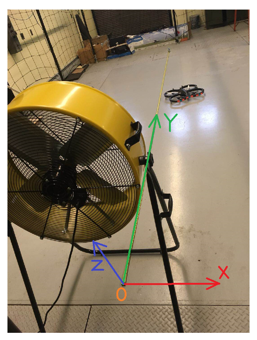
The coordinate system used in this work is shown in Figure 1. The origin O is defined at the projection of the center of the fan onto the ground. The Y axis points to the wind direction, the Z axis points upward, and the coordinate system follows the right-hand rule.
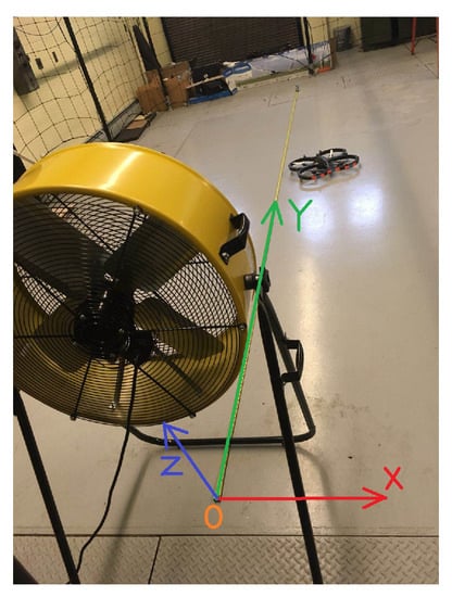
Figure 1.
Coordinate system set up.
2.5. The System
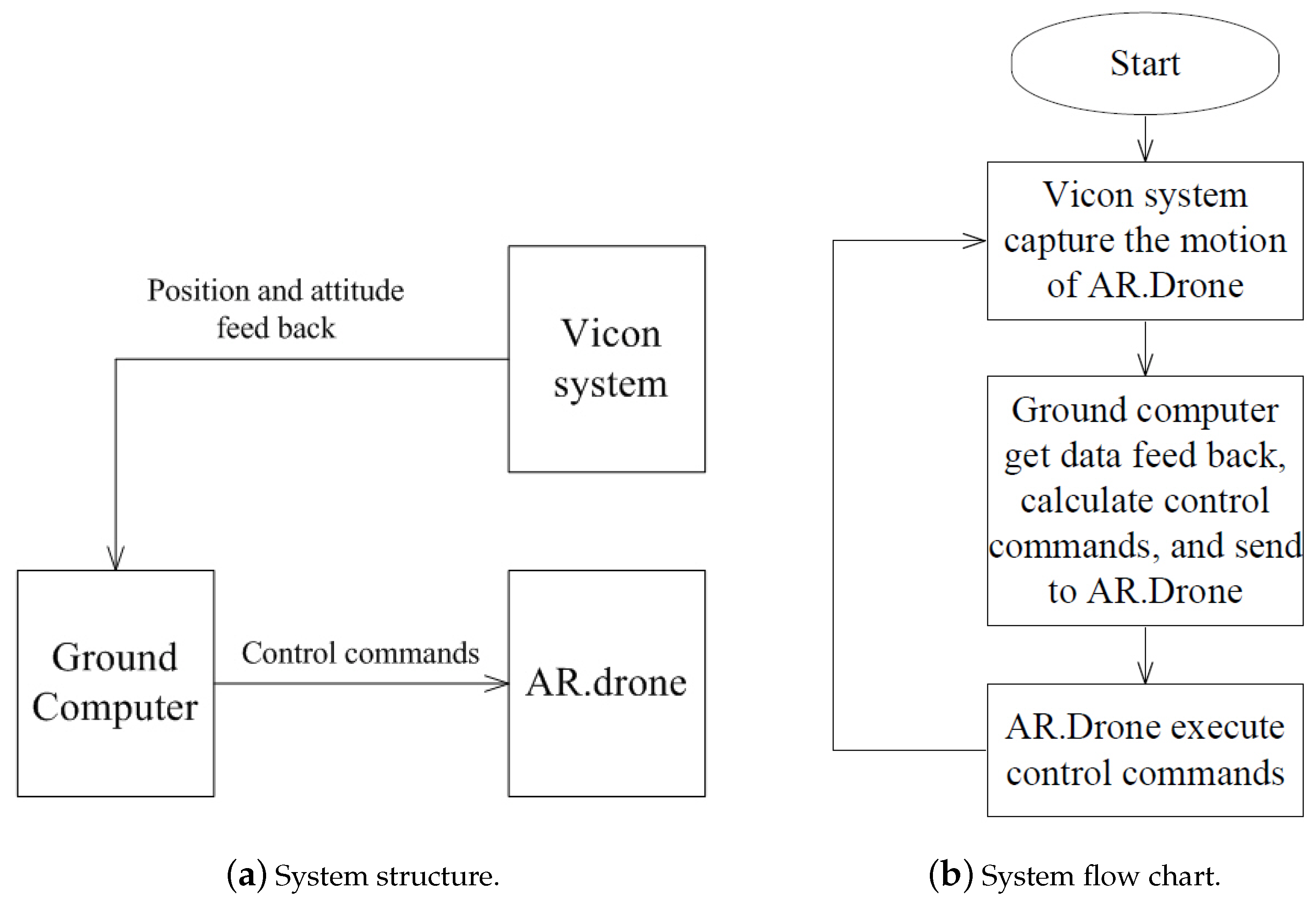
In this work, the Vicon camera system captures the motion of the AR.Drone, calculates AR.Drone’s positions x, y, z, attitude Euler angles roll, pitch, yaw (, , ), and sends these data to the ground computer. Based on these data, the ground computer runs the designed controller, and sends the calculated control commands , , , to the AR.Drone. Figure 2 shows the system structure and the system flow chart. In this work, the loop (show in Figure 2b) runs at 30 Hz. Since we keep sending the control commands from ground station at 30 Hz rate, the internal vision-based position hold using the bottom camera and sonar-based altitude hold algorithms of AR.Drone are not activated.
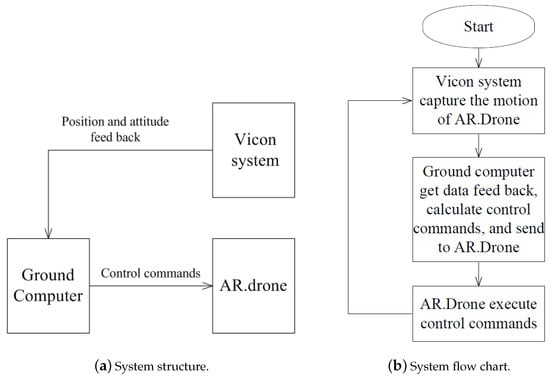
Figure 2.
System flow chart: (a) System structure and (b) System flow chart.
3. Data Curation
During this stage, we design a single set of PID controllers to hover the UAV across a range wind speeds. From the recorded flight data, we extract features that are related to the wind speed. Then, the extracted features and wind speed are saved in a database for wind estimation stage.
3.1. PID Control Law
A PID control method for discrete time systems is used in this work [16]. In general, let be the state measured in step k, be the desired state of step k, then the error at step k is
The summation of historical errors at step k is
The difference of error at step k is
Then the control input u at step k is defined as
where P, I, D are the gains of the PID controller.
In this work, we design four independent PID controllers for the four control channels by using the PID control law. The control channel (roll angle) is calculated based on the x error. The control channel (pitch angle) is calculated based on the y error. The control channel (yaw angular velocity) is calculated based on the yaw angle error. And the control channel (velocity of the altitude) is calculated based on the altitude error. For the control of yaw angle , the goal is to maintain it equal to , so the head of the drone will point along the y direction.
The four PID controllers are tuned under no wind condition. We use the Vicon data for feedback, set one point as the desired position, and tuned the gains P, I, and D to hover the drone at the point. The control cycle’s frequency is 50 Hz, and the unit of x, y and z error is in meters, the unit of yaw angular velocity is in degree per second. The result’s of the tuned gains we used are listed in Table 1.

Table 1.
PID gains we used.
After the gains are tuned, the values are used for later experiments. The controls are sent to AR.Drone through the SDK provided by the manufacturer. The mode of AR.Drone is set as non-hover mode, so the controls to the drone are purely from the controllers designed.
3.2. Flight Data Collection
Based on the size of the flight area (7 m by 4 m), the maximum wind speed generated by the fan (6 m/s), and the flight safety clearance (set to be m to the boundary of the flight zone), we select 8 wind speeds for training. The wind speed starts from 0 m/s and reaches maximum at m/s, with m/s increment.
For different wind speeds, we use the same PID controllers to hover the drone at the corresponding positions. For each flight, we command the drone hover for 30 s. Since the loop (Figure 2b) is run with 30 Hz, we collect 900 data points for each flight.
In each loop, we acquire six flight states from the Vicon system and 4 control commands from the PID controller. For the six flight states, we denote them as . And for the four control commands we denote them as . We denote the desired hover position as , , and . Then, we can define the position error as , , and . Because the desired attitude angles are all zero, the true attitude is the attitude error in this work. In each loop k, ten data points are recorded, and we denote them as:
3.3. Features
3.3.1. Features Definition
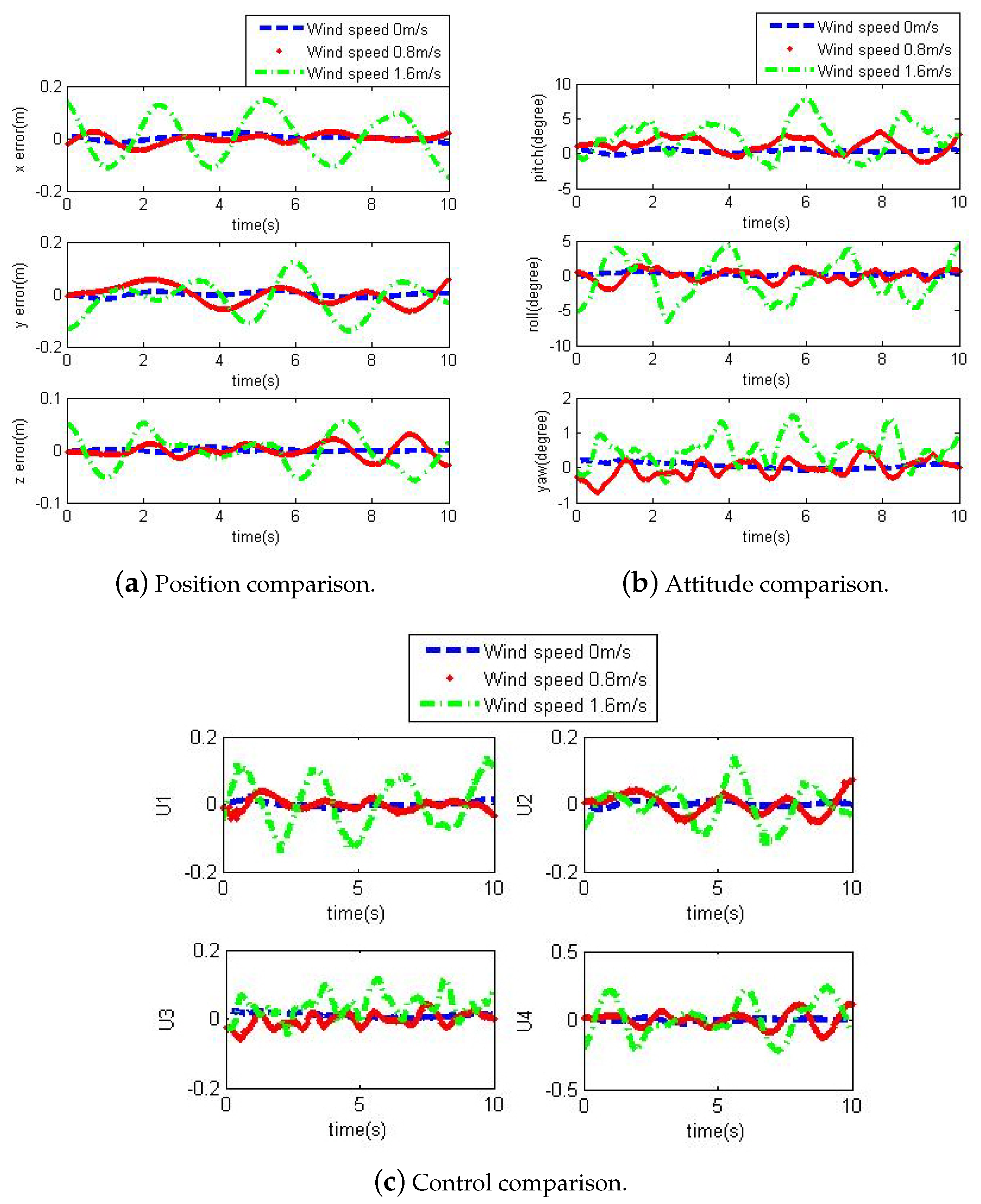
In this section we illustrate how we extract features from the flight data under each wind situation. Figure 3 shows the comparison of the hover performance for 10 s using the same PID controllers. In these figures, the blue dash represents the case that the wind speed is zero, the red dot represents the case that the wind speed is m/s, and the green dot dash represents the case that the wind speed is m/s. From the comparison, we can see that the wind will significantly affect the hover flight. When the wind speed increases, the position and attitude errors are increased, and the control efforts are also increased in order to maintain the hover flight.

Figure 3.
Control comparisoncomparisons: (a) Position comparison, (b) Attitude comparison and (c) Control comparison.
Based on our experience and observation, we choose 19 features which are highly related to the wind speed. The first seven features are related to the position error. They are the mean and variance of , , , and the mean of total position error. The total position error is defined as:
Similarly, the second seven features are related to the attitude. They are the mean and variance of the absolute values of the , , , and the mean of total attitude error. The total attitude error is defined as:
The last 5 features are related to the control effort. For the control, in programming, the scale is set from to 1, where 0 means the control effort is zero, and 1 means the maximum control efforts for opposite directions. In this work, the control effort is defined as the absolute value of the control commands, from 0 to 1. The five features we used are the mean control effort of , , , , and the total control effort. The total control effort C is defined as:
For each flight with the corresponding wind speed, we can analyze the flight data and calculate the feature vector. We denote the feature vector as:
where:
3.3.2. Features’ Effectiveness Validation
To validate that the designed features are effective, we check the Pearson-r coefficient [17] by using Python’s Seaborn library. Pearson-r coefficient indicates the correlation between two variables. It ranges from to 1. The sign of Pearson-r coefficient shows the two variables are positive correlated or negative correlated. When two variables are irrelevant, the corresponding Pearson-r coefficient is 0, and when two variables are highly correlated, the absolute value of Pearson-r coefficient is close to 1. It is expected for the values of the features to increase as the wind speed increases. In the tests for all 19 features respect to the wind speed, Pearson-r coefficients are observed larger than 0.5, thus proving the positive correlation between the feature vectors and the wind speed, and it also indicates that the 19 selected features are effective. Table A1 in Appendix A shows the results of the Pearson-r coefficient respect to the features.
3.4. Training Database Construction
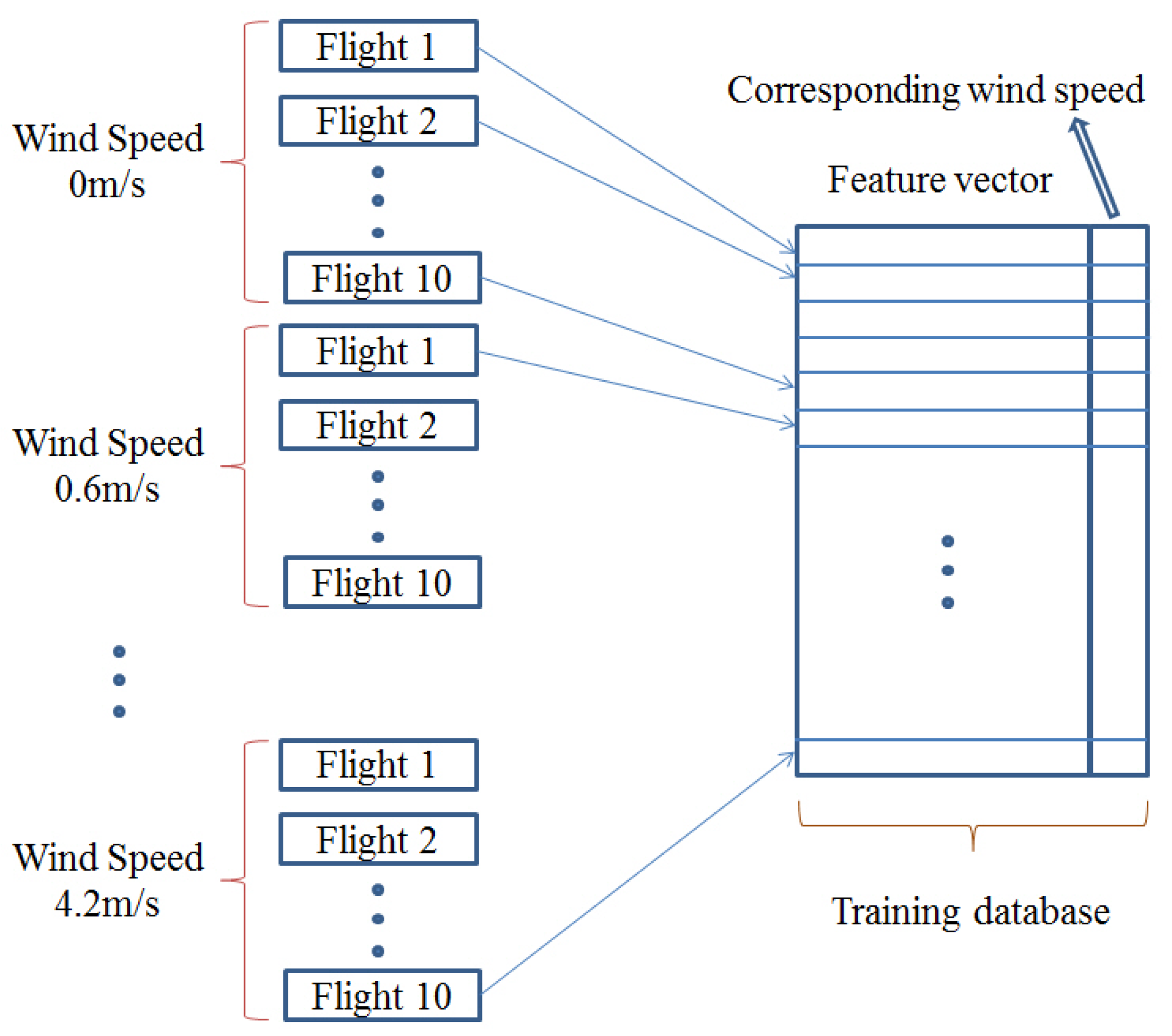
For each wind speed, we conduct ten independent flights and acquire ten feature vectors. In total, we have eight wind speeds, so we have 80 feature vectors stored. For each feature vector, we put the measured wind speed in the end. So we have a 80 by 20 matrix stored as the model. The row index i starts from 1 to 80, and the column index j starts from 1 to 20. When j is between 1 and 19, the data represents the feature, and when j is 20, the data represents the wind speed. Figure 4 illustrates the method to generate the database.
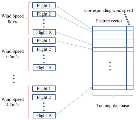
Figure 4.
Illustration of the method to generate the training database.
4. Wind Speed Estimation Stage
In this section, we introduce the KNN algorithm we used, including the feature normalization, distance calculation, and the wind speed calculation. Also, the strategy to choose the parameter K in KNN method is discussed.
4.1. KNN Algorithms
4.1.1. Feature Normalization
As we can see, the feature vectors are of different magnitudes and units. To compare the two features, we first normalize the features. We take feature as an example. Suppose that we have n independent experiment for training, and we have n feature . Now we have another flight experiment to estimate the wind for this flight, and have one more . In total, we have features. In the feature, we find the largest one , and the smallest one . Take the difference, we have . After that, each feature is divided by , and the results are the normalized features. We denote the normalized feature vector as F.
4.1.2. Distance Calculation
To compare the distance d of two normalized feature vectors and , we use the weighted Manhattan distance. The weighted Manhattan distance used in this work is defined as:
where w is the weight for each feature, which is equal to the Pearsonr coefficient which corresponds to the importance of the feature. The higher importance, the larger weight will be assigned.
4.1.3. Wind Speed Estimation
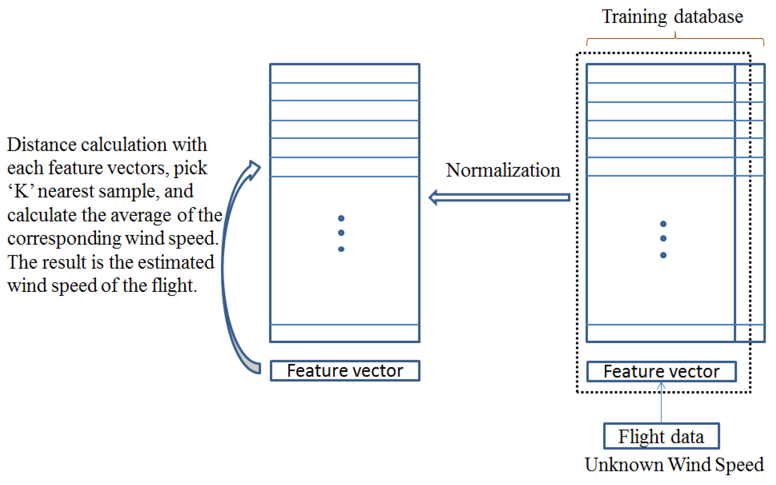
When there is a new flight, we can extract a 1 × 19 feature vector using the same method as we used during model generation. Then, we compare the feature vector with the 80 feature vectors in the model, and record its distance to each one in the model. Among the 80 distances, we choose K smallest ones, and get their row index i. After that, we look at the column 20, add the wind speed together and divided by K. The results will be the wind speed estimation for this flight. Figure 5 illustrates the method to calculate the wind speed.
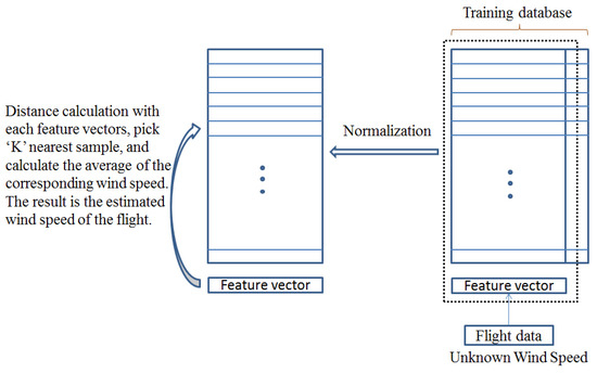
Figure 5.
Illustration of the method to calculate the wind speed.
4.2. Choose the Value of K
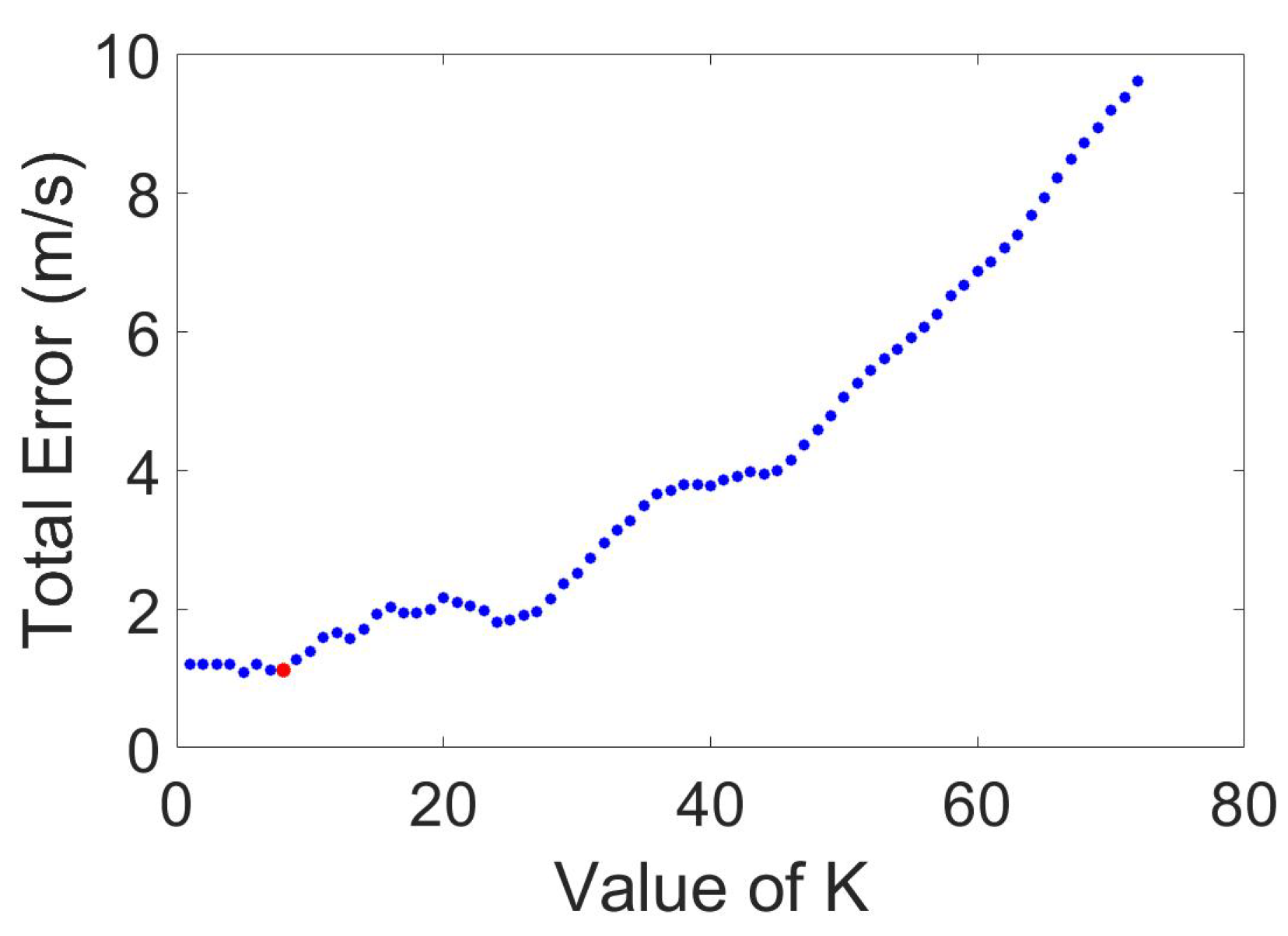
The parameter K is important for the KNN algorithm to work properly. When K is either too large or too small, the estimation result will not be reliable. As K is reduced, the fitting is better but the function becomes more complex, while as K increases, the function is smoother but less flexible and the training error increases. To find the appropriate value of K, we first test the KNN algorithm by using the model data.
For each wind speed, we randomly choose one of the ten experiments as the validation vectors, and the rest of the 9 remain as the model. In total, we will have 8 validation vectors, and 72 vectors as the model. For K value selection, we test it from 1 to 72, and find the best choice which leads to the minimum total estimation error of the eight experiments. The estimation error E is defined as:
where is the estimated wind speed, v is the wind speed reference. And the total estimation error is .
Figure 6 shows the total estimation error using different K. We can see that when , the total estimation error reaches the minimum. Because the ten validation data vectors are randomly chosen, the best value of K may not always be 8. We have repeated the experiment ten times, and the average of the best K value is 11. So we choose 11 as the value of the K for later experiments.

Figure 6.
Find the best K.
5. Experiment Results
To test the performance, in this section, we first introduce the wind field of the fan, then we compare the wind field estimation of our proposed method and the result from the AR.Drone. Users are allowed to subscribe a wind estimation topic directly in ROS, which is provided by the AR.Drone.
5.1. Wind Field Generation
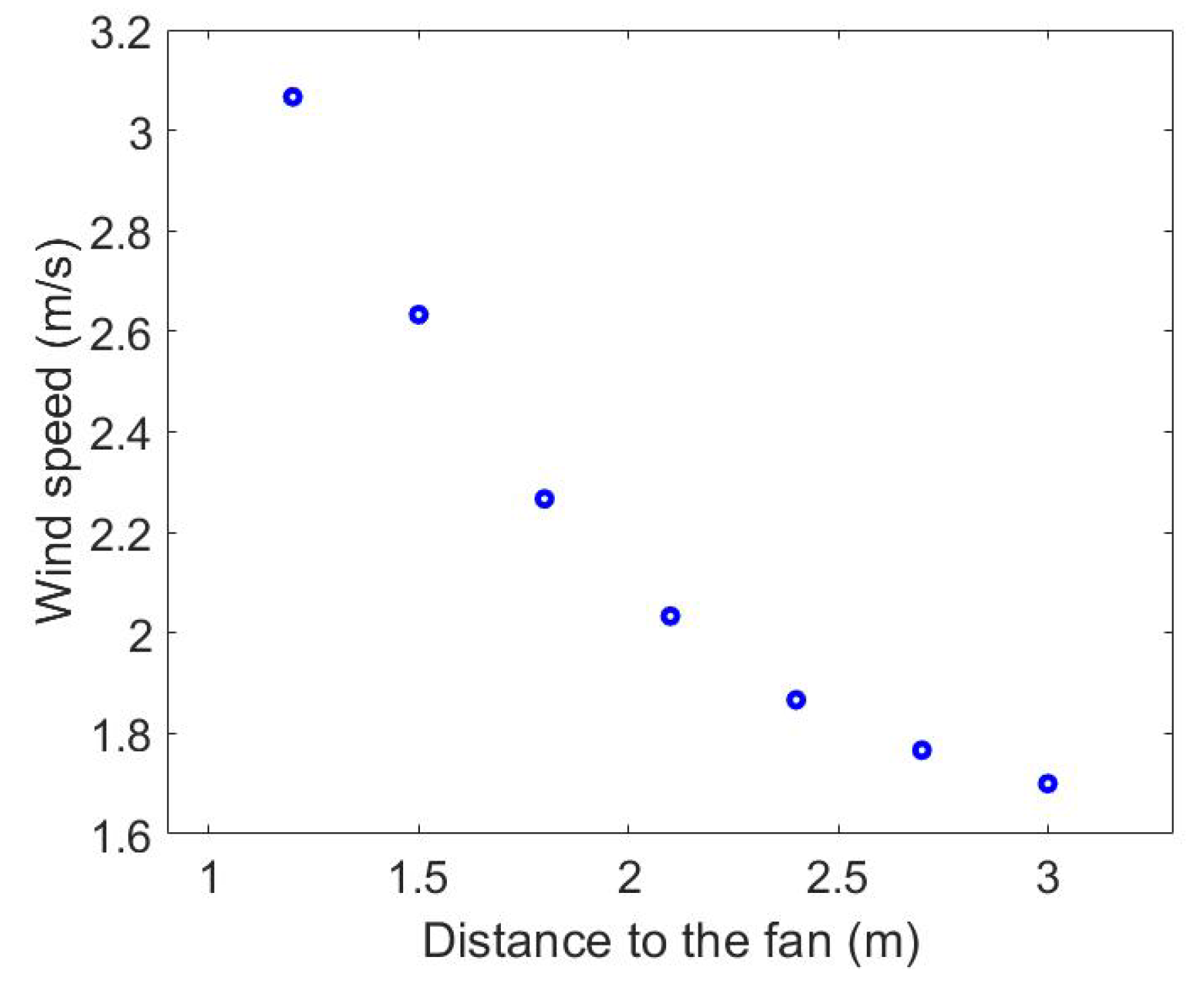
Based on the size of our lab, we choose seven points along the wind direction, and measure the wind speed at these points. The coordinate of these points are , , , , , , and . They are along the y axis and at the height of . At each position, we use the anemometer to measure the wind speed five times, and the average of the measurements is chosen as the reference wind speed at this point. Table 2 list the distance to the fan and the corresponding wind speed. Figure 7 shows the measured wind speed at these points.
Table 2.
Wind speed measurements and their corresponding distance to the fan.
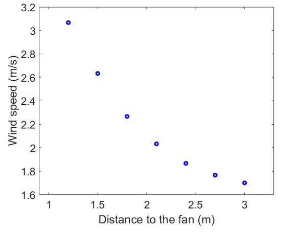
Figure 7.
Wind speed change as the distance to the fan change.
5.2. Wind Speed Estimation Results
We assign the way point over the seven positions, and hover the drone at each position for 20 s. Then, we use the saved database as the model, and choose to calculate the wind speed estimations. At the same time, the wind speed estimation results of from the AR.Drone embedded system are also recorded. We note that the wind estimation algorithms of AR.Drone are not available, so we only list the results as a reference. Table 3 and Figure 8 show the results of our proposed method and the result from the AR.Drone.
Table 3.
The comparison of our proposed method and the AR.Drone.
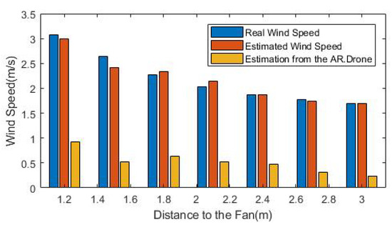
Figure 8.
On-line wind estimation results.
From the results, for the seven wind speeds, we calculate the estimation errors are m/s, m/s, m/s, m/s, m/s, m/s, and m/s, respectively. The average estimation error is m/s. And the estimation relative errors are , , , , , , and , respectively. The average estimation relative error is . At the same time, the average estimation error of the AR.Drone’s embedded system is m/s.
6. Conclusions
In this paper, a KNN-based wind estimation method for a rotary-wing VTOL UAV is presented. The proposed method uses the features generated by flight data as the learning model, and does not require the details of the aerodynamic information. Also, this method only uses flight data to generate the designed features for the training and wind estimation stages, and does not require direct wind speed measurements. Experimental results show that the proposed method can estimate the wind accurately, with a m/s average estimation error, and a average estimation relative error, while the average estimation error generated by AR.Drone’s embedded system is m/s. In future, our research will focus on wind direction estimation, and optimal selection of the features related to the wind direction will be studied. Future work will aim to focus on validation of the proposed algorithm in an outdoor environment.
Author Contributions
Conceptualization, L.W. and X.B.; methodology, L.W.; software, L.W.; validation, L.W. and G.M.; formal analysis, L.W. and X.B.; resources, L.W.; Data curation, L.W.; writing—original draft preparation, L.W.
Funding
The authors would acknowledge the research support from the Air Force Office of Scientific Research (AFOSR) FA9550-16-1-0814 and the Office of Naval Research (ONR) N00014-16-1-2729.
Conflicts of Interest
The authors declare no conflict of interest.
Appendix A
Table A1.
Features and the tested Pearson-r coefficients.
Table A1.
Features and the tested Pearson-r coefficients.
| Features | Pearson-r Coefficient |
|---|---|
| 0.92 | |
| 0.81 | |
| 0.87 | |
| 0.67 | |
| 0.86 | |
| 0.82 | |
| 0.95 | |
| 0.90 | |
| 0.82 | |
| 0.90 | |
| 0.85 | |
| 0.73 | |
| 0.58 | |
| 0.96 | |
| 0.92 | |
| 0.87 | |
| 0.81 | |
| 0.91 | |
| 0.94 |
References
- Galway, D.; Etele, J.; Fusina, G. Modeling of urban wind field effects on unmanned rotorcraft flight. J. Aircr. 2011, 48, 1613–1620. [Google Scholar] [CrossRef]
- Merino, L.; Caballero, F.; Martínez-de Dios, J.R.; Ferruz, J.; Ollero, A. A cooperative perception system for multiple UAVs: Application to automatic detection of forest fires. J. Field Robot. 2006, 23, 165–184. [Google Scholar] [CrossRef]
- Costa, F.G.; Ueyama, J.; Braun, T.; Pessin, G.; Osório, F.S.; Vargas, P.A. The use of unmanned aerial vehicles and wireless sensor network in agricultural applications. In Proceedings of the 2012 IEEE International Geoscience and Remote Sensing Symposium, Munich, Germany, 22–27 July 2012; pp. 5045–5048. [Google Scholar]
- Tan, Z.; Dong, J.; Xiao, Y.; Tu, J. A numerical study of diurnally varying surface temperature on flow patterns and pollutant dispersion in street canyons. Atmos. Environ. 2015, 104, 217–227. [Google Scholar] [CrossRef]
- Pan, C.X.; Zhang, J.Z.; Ren, L.F.; Shan, Y. Effects of rotor downwash on exhaust plume flow and helicopter infrared signature. Appl. Therm. Eng. 2014, 65, 135–149. [Google Scholar] [CrossRef]
- Prudden, S.; Fisher, A.; Marino, M.; Mohamed, A.; Watkins, S.; Wild, G. Measuring wind with Small Unmanned Aircraft Systems. J. Wind Eng. Ind. Aerodyn. 2018, 176, 197–210. [Google Scholar] [CrossRef]
- Lusardi, J.A.; Tischler, M.B.; Blanken, C.L.; Labows, S.J. Empirically derived helicopter response model and control system requirements for flight in turbulence. J. Am. Helicopter Soc. 2004, 49, 340–349. [Google Scholar] [CrossRef]
- Divitiis, N.D. Wind estimation on a lightweight vertical-takeoff-and-landing uninhabited vehicle. J. Aircr. 2003, 40, 759–767. [Google Scholar] [CrossRef]
- Velasco-Carrau, J.; García-Nieto, S.; Salcedo, J.; Bishop, R.H. Multi-objective optimization for wind estimation and aircraft model identification. J. Guid. Control. Dyn. 2015, 39, 372–389. [Google Scholar] [CrossRef]
- Pappu, S.; Liu, Y.; Horn, J.F.; Copper, J. Wind Gust Estimation on a Small VTOL UAV. In Proceedings of the AHS Technical Meeting on VTOL Unmanned Aircraft Systems and Autonomy, Mesa, AZ, USA, 24–26 January 2017. [Google Scholar]
- Sikkel, L.; de Croon, G.; De Wagter, C.; Chu, Q. A novel online model-based wind estimation approach for quadrotor micro air vehicles using low cost MEMS IMUs. In Proceedings of the 2016 IEEE/RSJ International Conference on Intelligent Robots and Systems (IROS), Daejeon, Korea, 9–14 October 2016; pp. 2141–2146. [Google Scholar]
- Larose, D.T. k-nearest neighbor algorithm. In Discovering Knowledge in Data: An Introduction to Data Mining; John Wiley & Sons: Hoboken, NJ, USA, 2005; pp. 90–106. [Google Scholar]
- Chaves, S.M.; Wolcott, R.W.; Eustice, R.M. NEEC Research: Toward GPS-denied landing of unmanned aerial vehicles on ships at sea. Nav. Eng. J. 2015, 127, 23–35. [Google Scholar]
- Krajník, T.; Vonásek, V.; Fišer, D.; Faigl, J. AR-drone as a platform for robotic research and education. In International Conference on Research and Education in Robotics; Springer: Berlin/Heidelberg, Germany, 2011; pp. 172–186. [Google Scholar]
- Windolf, M.; Götzen, N.; Morlock, M. Systematic accuracy and precision analysis of video motion capturing systems—exemplified on the Vicon-460 system. J. Biomech. 2008, 41, 2776–2780. [Google Scholar] [CrossRef] [PubMed]
- Wang, L.; Bai, X. Quadrotor Autonomous Approaching and Landing on a Vessel Deck. J. Intell. Robot. Syst. 2017, 92, 125–143. [Google Scholar] [CrossRef]
- McGraw, K.O.; Wong, S.P. Forming inferences about some intraclass correlation coefficients. Psychol. Methods 1996, 1, 30. [Google Scholar] [CrossRef]

© 2019 by the authors. Licensee MDPI, Basel, Switzerland. This article is an open access article distributed under the terms and conditions of the Creative Commons Attribution (CC BY) license (http://creativecommons.org/licenses/by/4.0/).