1. Introduction
The Midlands region forms the primary agricultural region within the Australian State of Tasmania. The region was once populated by expanses of native grasslands and open woodlands [
1]. However, these communities have seen a significant decline since European colonization began. Throughout subsequent years, native vegetation has been replaced by traditional European crop and forage species as agricultural land use in the region intensifies. Native vegetation communities still remain in the region, and are often used for grazing of sheep and cattle. However, the economic return associated with native grassland grazing is poorer than for introduced pasture species due to a lower nutritional value within the vegetation [
2]. As a result, native grassland community extent has been steadily declining. Although the exact extent of native grassland vegetation lost is unknown, the estimated loss of community extent is estimated to be between 60% [
3] and 90% [
4] of a pre-colonial extent.
Collectively, the major grassland community types of the region are known as the lowland native grasslands. These communities form the Midlands biodiversity ‘hotspot’ [
4], and contain an estimated 750 species, of which 85 are protected under Tasmanian or Federal Australian environmental protection laws [
2,
5]. The high level of biodiversity within these communities, coupled with the major threat of habitat loss due to expanding agricultural practices, has created a desperate need for novel approaches to mapping and monitoring of vegetation communities in the region. Community maps of native vegetation within the Midlands region are often incomplete or outdated [
6], and, as a result, remote sensing has been proposed as a potential answer, due to its ability to provide frequently updateable maps of vegetation community extent and condition. However, due to the small patch size of remnant communities [
4], coarse spatial resolution satellite-based approaches have proven to be moderately successful [
7]. The rise of Unmanned Aerial Systems (UAS) in recent years, therefore, provides a unique opportunity to capture ultra-high spatial resolution data products that can be used to improve upon currently existing mapping approaches in the region.
The application of Unmanned Aircraft Systems (UAS) for environmental remote sensing applications has become increasingly prevalent in recent years. The ability of UAS to provide ultra-high spatial resolution datasets (<20 cm pixel size) at a relatively low cost makes them an attractive option for many researchers in this field [
8]. The development of commercially available, ‘off the shelf’ platforms has led to a rapid increase in the applications for which UAS have been used in environmental sciences. The applicability of UAS for grassland monitoring and mapping is particularly attractive due to the ability of such systems to collect spatially detailed datasets on demand. This ability is integral to grassland remote sensing due to the high seasonal variability observed in communities [
9,
10,
11].
Several studies have employed UAS as the principle platform in grassland research [
12,
13,
14]. Although applications are primarily focussed on small-scale studies of agricultural productivity, such as estimating biomass [
15], several studies have focussed on broader-scale ecological applications of UAS for various applications within grassland environments such as monitoring degradation and change [
16], mapping species regeneration post-fire [
17], estimating ground cover in rangelands [
18], identifying grassland vegetation [
19], and assessing species composition [
13]. The most prevalent area of grassland research using UAS, however, is for rangeland monitoring and mapping. Extensive work has been undertaken, particularly in the South Western United States, to determine the feasibility of UAS for broad-scale, high spatial resolution analysis of semi-arid grassland and shrub communities [
14,
20,
21].
The majority of remote sensing studies using UAS within the realm of ecological research have focused on the use of ultra-high spatial resolution datasets collected using broadband multispectral sensors [
22] or RGB cameras [
16] due to their low cost [
8]. The use of broadband multispectral sensors is not always capable of providing sufficient spectral detail for accurate analysis of vegetation types and attributes, even when the data are acquired at high spatial resolutions. Applications of hyperspectral sensors using UAS platforms are still limited in general. However, there is an increasing body of work investigating their applicability in fields such as precision agriculture [
23,
24,
25,
26,
27,
28]. Due to the fact that the majority of previously available high spectral resolution sensors are based on push broom designs, the high fidelity Global Navigation Satellite System (GNSS) and Inertial Measurement Unit data were required for the creation of useable outputs [
23,
29]. This issue has led to limited use and application of UAS mounted hyperspectral sensors within the ecological remote sensing community. The development of frame-based and snapshot hyperspectral cameras, however, eliminates the need for complicated geometric processing, and makes the collection of hyperspectral datasets from UAS much more feasible. The use of such sensors has enormous potential for ecological vegetation mapping and monitoring due to the high degree of spectral information captured. This study aims to show the potential of a frame-based hyperspectral system for the vegetation community mapping in a highly heterogeneous grassland environment. Previous studies [
7,
30] in the area have identified a need to investigate the utility of hyperspectral systems in such environments, and this study aims to provide an important test case to improve lowland grassland community mapping through the use of novel sensor technologies.
2. Materials and Methods
2.1. Study Site and Vegetation Communities
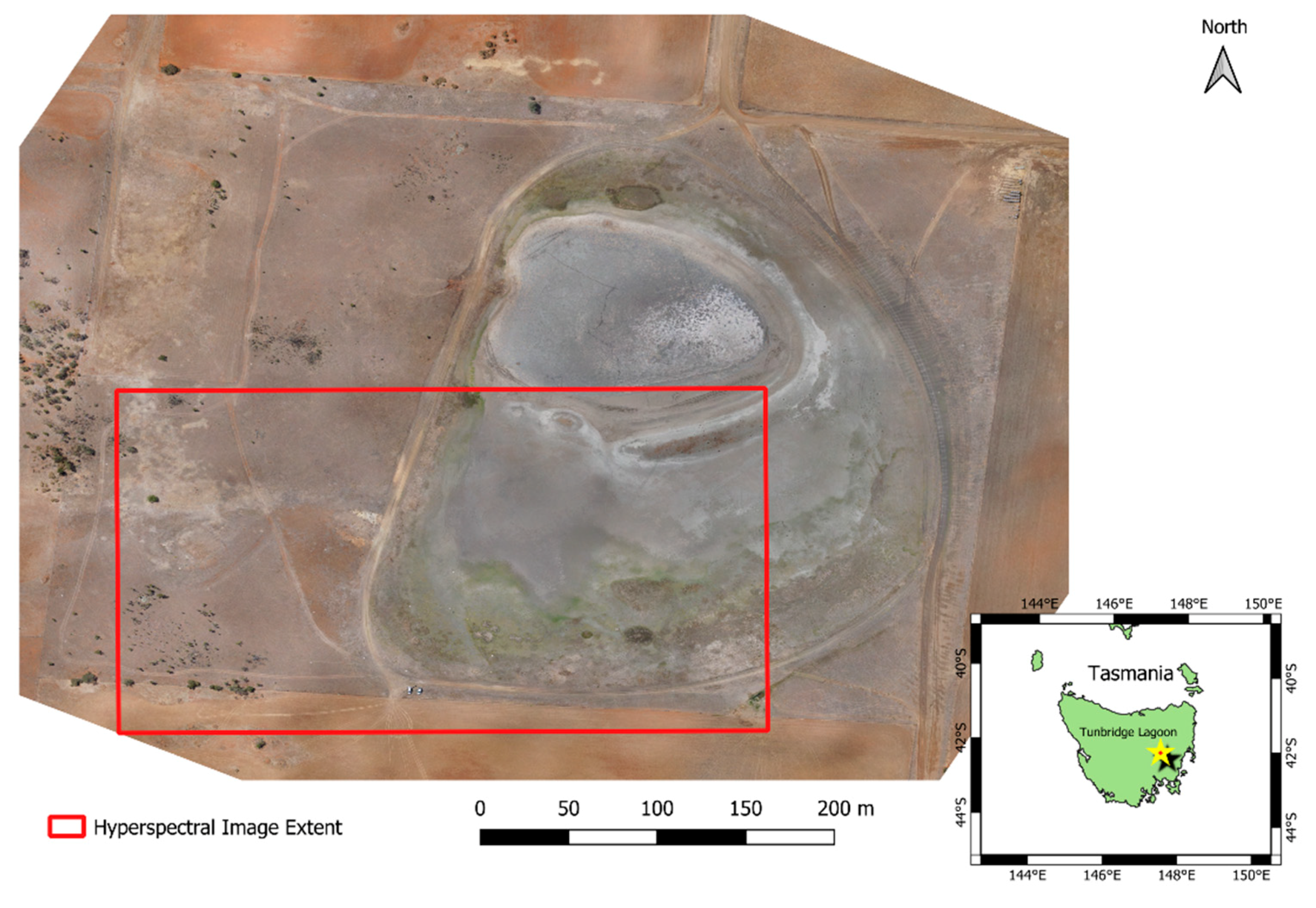
In November 2015, imagery was collected at the Tunbridge Township Lagoon (42°08′52.36″, 147°25′45.50″), in the Tasmanian Midlands. The town of Tunbridge is located between the two major settlements of Hobart and Launceston, and marks the divide between the Northern and Southern Midlands regions. The lagoon serves as the only formally protected lowland native grassland habitat in Tasmania, and contains important remnant vegetation patches and many endangered species. The reserve covers an area of approximately 16 ha, and has wide floristic diversity. The western third of the site is populated by remnant Themeda triandra grassland and interspersed with Acacia dealbata and Bursaria spinosa. This portion of the site is steeply sloped in an easterly aspect. The remaining two thirds of the site are predominantly flat, and covered with a saltwater lagoon. The saltpan surrounding the lagoon is populated by many saline tolerant ground cover species, such as Wilsonia rotundifolia, Sellieria radicans, and, in places, the Australian Saltmarsh grass Puccinellia stricta. The areas between the saltpan and the bounding western and southern fences are populated by remnant Danthonia trenuior and Poa labillardierie grasslands. Vegetation communities are generally in good condition, although the southern side of the lagoon and a small area at the foot of the hill immediately adjacent to the lagoon is still recovering from unplanned burning in the summer of 2014.
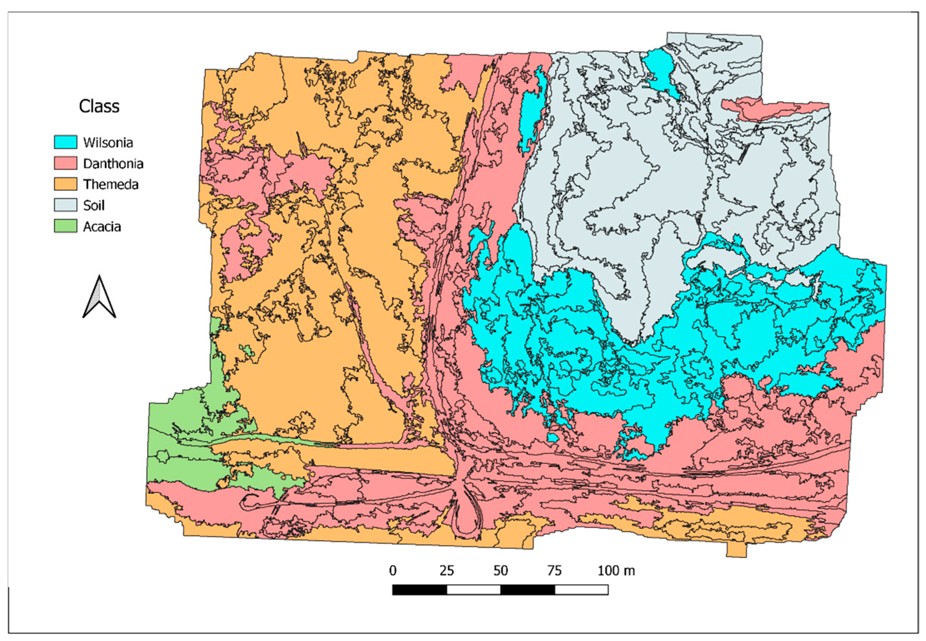
For the purpose of this study, a subset of the total reserve area was targeted. This area is found on the south-western corner of the lagoon, and covers a transitional area between saltmarsh vegetation, native grassland communities dominated by Danthonia trenuior or Poa labillardierei, and the foot of the hill dominated by Themeda triandra. A total of four vegetation classes were identified for analysis, as well as a soil class. The first class consists of the saline vegetation communities found surrounding the lake including the succulent Selliera radicans and the ground cover Wilsonia rotundifolia. The second class covers the range of native grassland communities adjacent to the lagoon, which are called Danthonia trenuior and Poa labillardierie dominated areas. The common feature among these communities is that they all follow the C3 photosynthetic pathway. The third class covers the Themeda triandra remnant patches found on the western slopes of the site. The fourth class is representative of the scattered Acacia and Bursaria specimens found among the Themeda grassland, and the final class consists of exposed soils found within the lagoon.
2.2. Data Collection
Data was collected using a multi-rotor UAS (DJI S1000) for hyperspectral imagery, and a fixed-wing UAS (Phantom FX-61) for RGB imagery. Hyperspectral imagery was collected using a PhotonFocus MV1-D2048x1088-HS02-96-G2-10 (
www.photonfocus.com), which is a 25 band hyperspectral snapshot camera, with a spectral wavelength range from 600 to 875 nm and average FWHM (Full-width Half Maximum) of 6 nm. The wavelength range of the camera was selected based on previous research identifying this spectral region as containing key areas of separability for lowland native grassland communities [
7,
30]. The camera houses a hyperspectral chip manufactured by IMEC with 25 band-pass filters mounted on top of the sensor’s pixels in a 5 × 5 mosaic pattern. The 25 bands are captured simultaneously and the pixels are organised in a hypercube of 409 by 216 pixels, and resampled to 20 bands after spectral correction.
Table 1 gives the central wavelength for each of the 20 bands. The camera captured images at 4 frames per second (fps). We used a 16 mm focal length lens providing a field of view of 39° and 21° horizontal and vertical, respectively. The camera was mounted on a gimbal on a DJI S1000 multi-rotor UAS, and flown in a grid survey pattern at 80 m above ground level with a flight line separation of 22 m providing 60% side overlap between flight strips and 97% forward overlap. The ground sampling distance (GSD) of the raw imagery was 3 cm, but, after spatial and spectral resampling, this was reduced to 15 cm. The flight track was recorded with a navigation-grade global navigation satellite system (GNSS) receiver (zti communications Z050 timing and navigation module, spatial accuracy 5–10 m), and each hyperspectral image frame was geotagged based on GPS time. One hundred images were captured before the flight with the lens cap on the camera and averaged to collect a dark current image. Another 100 images were captured on the ground of a Spectralon panel directly before and after UAS flights to apply a vignetting lens correction and to allow for conversion of DN values to reflectance. A Python script was developed to process the raw camera data into hypercubes with reflectance values. The resulting images were exported to the GeoTiff format and imported into AgiSoft Photoscan (with their corresponding GPS coordinates). The Structure from Motion (SfM), dense matching, model generation, and orthophoto generation processing steps were performed in a Photoscan based on band 14 (801 nm). Additionally, 22 photogrammetric ground control points were randomly distributed across the study site and coordinated with a dual frequency geodetic-grade RTK GNSS receiver (Leica 1200), which resulted in an absolute accuracy of 2 to 4 cm. A 348 m by 255 m hyperspectral ortho-mosaic of the full scene was produced for further analysis. Sky conditions were clear and sunny during all UAS flights. The hyperspectral flights occurred during a one-hour time window around solar noon.
Figure 1 shows an overview of the study site using the RGB UAV imagery, as well as the footprint of the hyperspectral dataset.
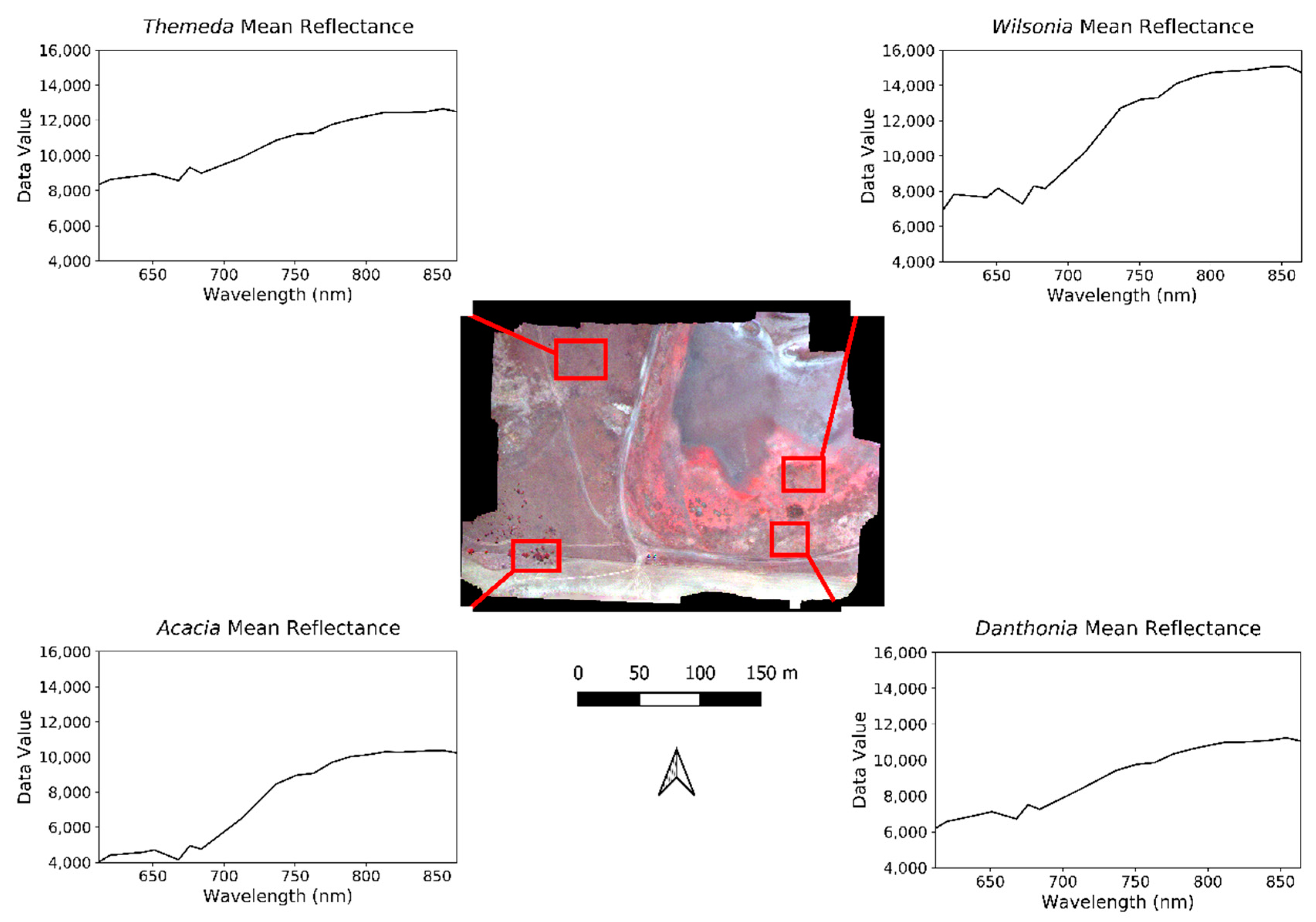
Figure 2 shows the hyperspectral orthophoto loaded as a false-color RGB composite using bands 14, 5, and 1 (801.7 nm, 668.1 nm, and 612.8 nm). Reflectance values are shown for the subset areas of each class.
Additionally, an RGB camera was flown on a fixed-wing UAS at a height of 80 m (Sony alpha 5100, 20 mm focal length lens, FOV = 60° × 43°, shutter speed 1/1000 s, GSD = 1.7 cm, forward overlap 80%, side overlap: 70%). An RGB orthophoto mosaic was produced 1.7 cm spatial resolution in Agisoft Photoscan using the SfM workflow described earlier. The Ground Control Points (GCPs) were used in the bundle adjustment, which produced an RGB orthophoto mosaic with an absolute spatial accuracy of 2 cm. A 15 cm spatial resolution digital surface model (DSM) was derived from the 3D dense point cloud and triangulated model. From this DSM, the slope was derived using the surface toolset in ArcGIS 10.3 [
31]. The RGB DSM and Slope model were used in the analysis over the hyperspectral outputs due to a better horizontal and vertical accuracy.
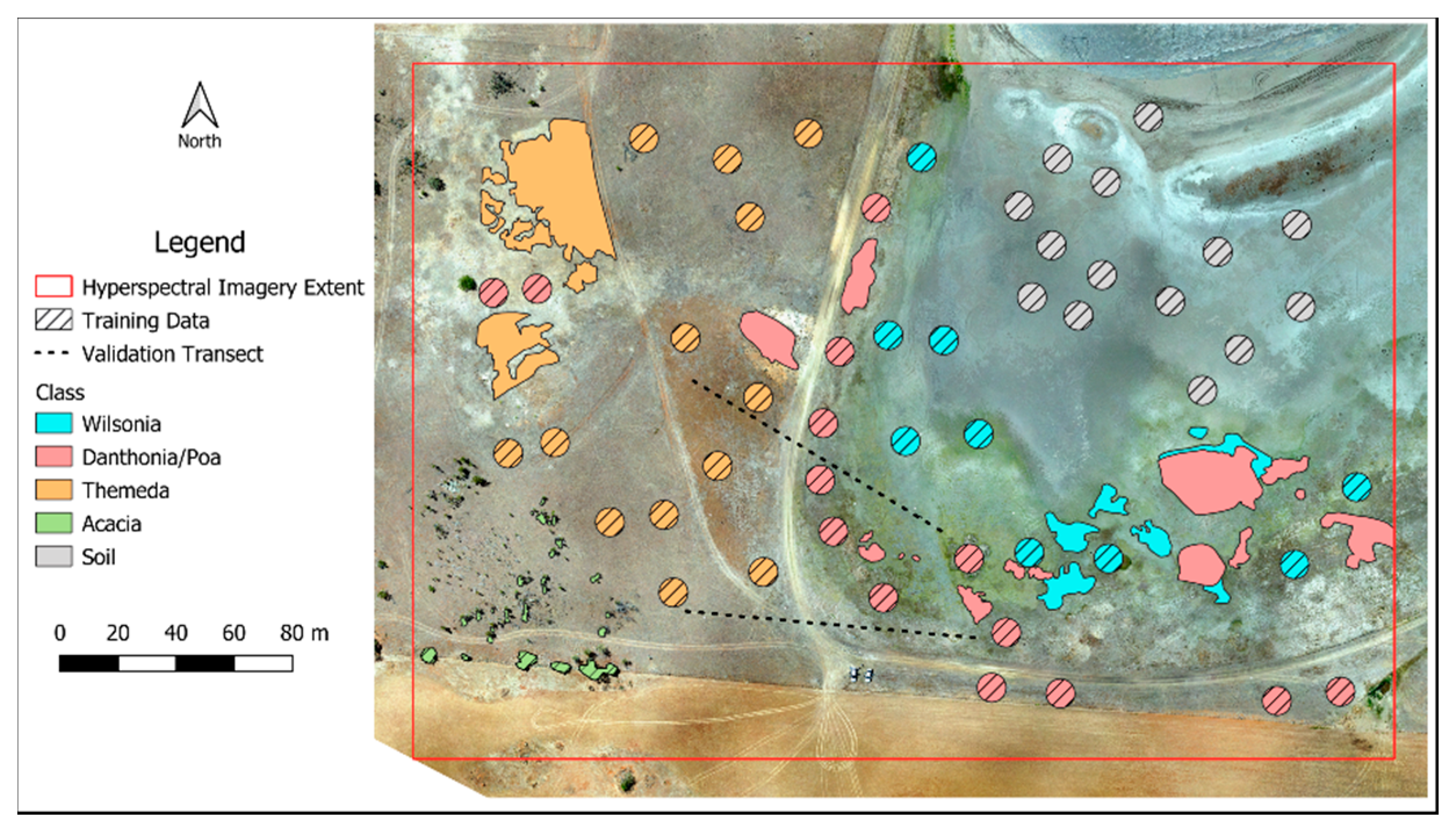
For validation purposes, two 100 m transects, as shown in
Figure 3, were established at the site during aerial data acquisition. The transects covered the
Wilsonia, Danthonia, and
Themeda classes over an area in which the communities intergrade significantly. Transects were run east to west across the center of the study area. Observations of plant communities were taken every meter along each transect. A polygon representing the observation area was then digitized in ArcGIS 10.3 for each point along the transect, and assigned the relevant class based on the field observations. Training points for the classification model were based on field observations acquired from 5 × 5 meter transects established in November and December 2015. Transect centroids were generated based on random stratification within the site and the coordinates of ground control points used for the UAS data acquisition. For each transect, a tape measure was aligned north to south, and the vegetation community was recorded every 1.25 m along the tape for a total of five observations. Observations were then taken east to west every 2.5 m, for nine observations. The majority vegetation community for the transect area was then determined and used as the classification label. For each transect centroid, a GPS coordinate was acquired, and imported into ArcGIS 10.3. Based on each point, a five meter buffer was generated and a series of points spaced 15 cm apart were generated within the bounds of the buffer zone. Furthermore, 15 cm was selected as the point spacing since this matched the spatial resolution of the final ortho-mosaic generated from the UAS dataset. Vegetation classes were assumed to be uniform within the entire 5 m zone, and care was taken to ensure that no transitional transects were used for training purposes.
Lastly, a set of reference segments representing homogeneous class regions were digitized for the four vegetation classes to serve as additional validation. Object size varied relative to class extent, which was between 1 m
2 and 100 m
2. Additional validation data was manually digitized in order to create an adequate sample size for classification validation and because there were no recorded observations for the
Acacia class, based on the 100 m transects. It was found that the two 100 m transects failed to provide an appropriate number of validation points for some vegetation classes.
Figure 3 shows the distribution of the 5 m buffered training zones, the validation transects, and manually digitized reference polygons within the study site.
2.3. Random Forest Training and Classification
Image segmentation was performed using the Multiresolution Segmentation Algorithm [
32] in eCognition based on the 20 spectral bands of the orthomosaic, the DSM, and the slope model. A scale factor of 1700 was used, with the compaction factor set to 0.1, and the shape factor set to 0.9. The DSM and slope model were included in the classification approach since they were previously found to be of high importance for classification of these communities [
7]. The DSM was not converted to a canopy height model due to the low height of vegetation in some sites of the study area (<1 cm in some areas). Once the segmentation had been completed, a random forest model was trained for classification. Training and classification were performed on the 20 band ortho-mosaic, the DSM, and the slope layers. Since the number of input variables was equal to 22, the number of variables to try (mtry) was set equal to 4, since the established optimal parameter value is equal to √m, where m is the number of variables used [
33,
34]. Internal cross-validation accuracies were obtained for the model, in addition to variable importance measures. Validation of the classification results was performed twice including once using the digitised reference objects, and a second time based on the 100 m transects. The reference objects and transects were not merged into a single validation dataset due to the difference in the scale of analysis between the two datasets. Merging the transect observation areas into the larger reference segment area would, therefore, result in this fine spatial scale of the observations being lost due to the large discrepancy in the area of analysis between the two datasets. Validation was performed using the reference segments in order to provide a large-scale estimate of accuracy across the entire scene, and also to ensure that an adequate number of validation points was used for each class. Validation using homogeneous reference segments also enables the evaluation of misclassification due to over-segmentation. The field transects were used as a secondary source of validation since they provide valuable data about the sensitivity of the sensor and classification results to transitional zones between communities. The high spatial frequency of observations along the transects allows for accurate determination of the exact point of change between vegetation types. Since community intergrading has been identified previously as being a significant source of classification confusion for these communities [
7], the decision was made to collect data capable of evaluating the sensitivity of the segmentation scale and classification approaches.
4. Discussion
The accuracies obtained for the RF training model are much higher than the accuracies obtained for any of the final classification results. The presence of significant discrepancies between validation and training accuracies can indicate potential bias in the sampling regime, or unrepresentative training datasets. Since the number of input points was high (~250,000), it was decided that a single RF model was to be derived. The high spatial resolution of the dataset (14 cm) means that very fine-scale variations in species composition can potentially be detected. Since training points were derived over a 5 m plot area to emulate the conditions, there is potential to incorporate multiple thematic classes within a single plot. Conversely, however, the use of small numbers of widely dispersed pixels may lead to a failure to properly account for class variability in the training and classification stages of analysis.
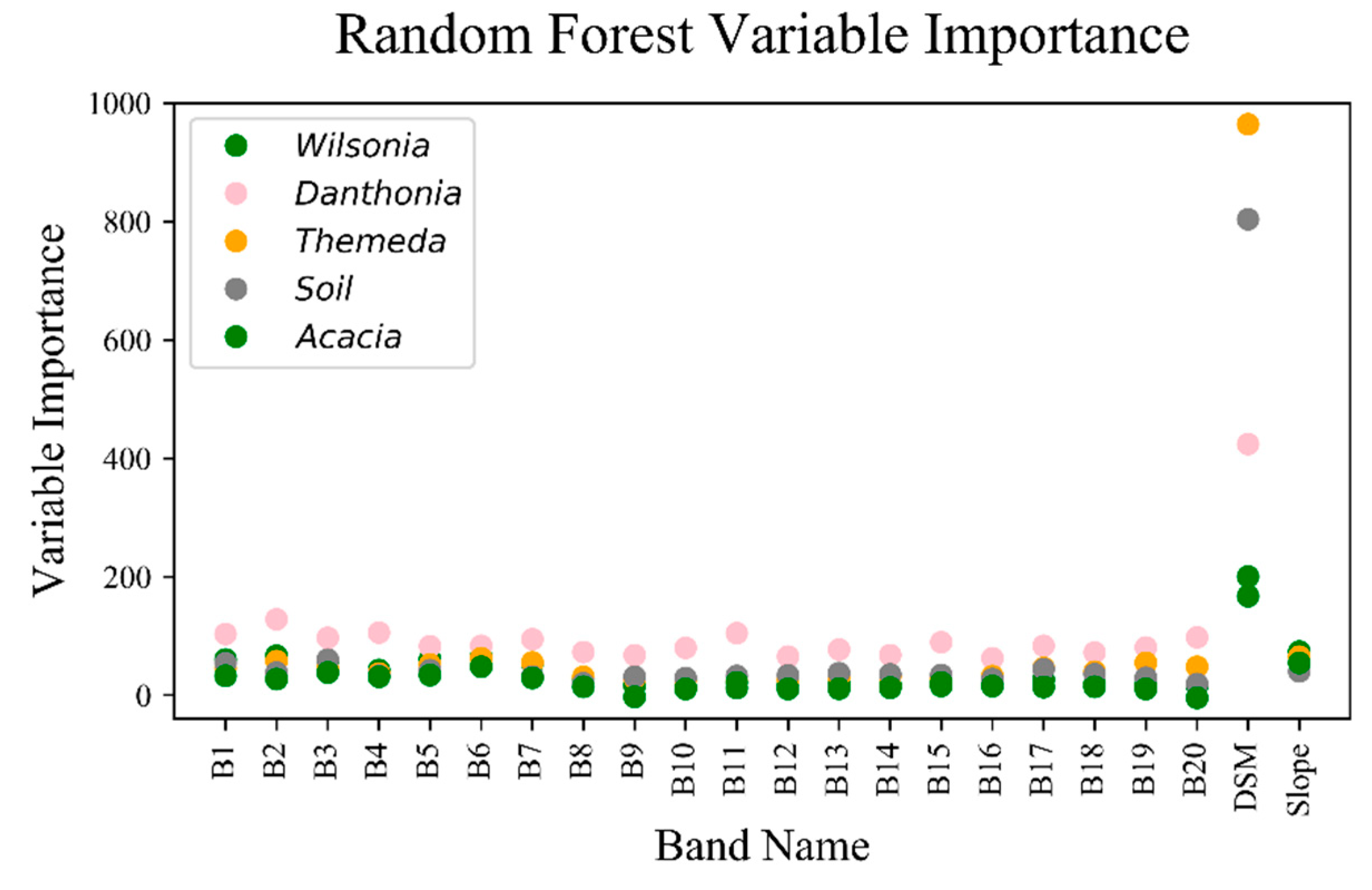
The variable importance measures obtained show a very high importance for the two topographic variables. Spectral variables have significantly lower importance values for each class, and all classes have their highest importance level recorded for the DSM. The high importance value assigned to the DSM in the Themeda class is due to the class occurring exclusively on the hilly area within the study site, whereas the Danthonia and Wilsonia classes occur on the flat saltpan surrounding the lagoon. This difference is of key importance due to similarities in the canopy structure between the Themeda and Danthonia classes, which may potentially lead to confusion between the two classes during classification.
Classes exhibit different importance levels across the range of spectral input bands, with the
Danthonia class having the highest overall spectral importance values. Key bands of importance for this class include band two (620.9 nm), 11 (763.2 nm), and 14 (801.7 nm). The observed regions of importance align with those identified in previous research [
7]. All other vegetation classes have comparatively low spectral importance values. Low importance values for the spectral variables is likely a result of high correlation between the bands. The high values for spectral bands in the
Danthonia result is likely due to similarities between the physical distribution of the
Danthonia and
Wilsonia classes, since both only occur on the same flat region of the saltpan. Since these two classes intergrade significantly, and cannot be differentiated based on topography, spectral bands are the only available source for differentiation with the RF model. This is likely to contribute to the poor performance of the class overall since previous studies undertaken at this site indicate great difficulty discerning between the
Danthonia and
Wilsonia classes due to their similar photosynthetic pathway and phenological staging [
30].
The primary source of inaccuracy in the classification results was confusion between the Danthonia and Wilsonia classes. The confusion in this case was only in one direction, in that a large proportion of the Danthonia class was erroneously classified as Wilsonia, while there was very little misclassification of Wilsonia as Danthonia. As the two communities intergrade extensively, the establishment of discrete reference objects for validation was very difficult even within the two 100 meter transects. Inaccuracy when creating these reference objects is likely to be the case of the poor overall accuracy obtained for the Danthonia class. Since the two classes occur in the same geographic area, primarily on low-lying saltpan, the DSM and slope variables are not likely to increase separability between the two classes. The Danthonia class exhibits significantly different final classification accuracies between the validation performed using the reference objects and the validation based on the image transects. The observed differences in classification accuracies between assessments based on the validation transects and manually digitized objects indicate that there is a need to collect high spatial resolution validation datasets in order to accurately assess the performance of classifications in this case.
This paper shows that discrimination between similar vegetation communities can be successful using hyperspectral, frame-based UAS mounted sensors. The spectral range of the sensor used in this case is quite narrow, with bands only covering the red and near-infrared portions of the spectrum from 600 to 875 nm. The use of a sensor with an expanded range into the visible portion of the spectrum may potentially improve classification outcomes, due to an increased ability to detect unique spectral properties of communities. The ability of the sensor to successfully discriminate between communities is most apparent in the results of the two grassland communities. The main difference between these communities is that they have different photosynthetic pathways. Many studies have shown that differentiation of grassland species based on photosynthetic pathway and phenological variation is an appropriate method [
35,
36]. The dataset used in this scenario was acquired at a time of year where the
Themeda grassland was entering a period of senescence, and the
Danthonia/Poa grassland was beginning its annual growth cycle. The results shown in this paper reiterate the findings of previous studies that have shown that phenology is a critical component of the grassland community identification. The overall findings of this paper suggest that frame-based hyperspectral UAS mounted sensors can be used to successfully differentiate between native grassland communities with a high degree of accuracy.


