Article

A Generalized Simulation Framework for Tethered Remotely Operated Vehicles in Realistic Underwater Environments

Computer Science and Software Engineering, University of Canterbury, Christchurch 8140, New Zealand
*
Author to whom correspondence should be addressed.
Submission received: 28 November 2018 / Revised: 17 December 2018 / Accepted: 19 December 2018 / Published: 21 December 2018

Abstract

:
This paper presents a framework for simulating visually realistic motion of underwater Remotely Operated Vehicles (ROVs) in highly complex models of aquatic environments. The models include a wide range of objects such as rocks, fish and marine plankton in addition to an ROV tether. A modified cable simulation for the underwater physical conditions has been developed for a tethered ROV. The simulation framework also incorporates models for low visibility conditions and intrinsic camera effects unique to the underwater environment. The visual models were implemented using the Unreal Engine 4 realistic game engine to be part of the presented framework. We developed a generalized method for implementing an ROV dynamics model and this method serves as a highly configurable component inside our framework. In this paper, we explore the unique characteristics of underwater simulation and the specialized models we developed for that environment. We use computer vision algorithms for feature extraction and feature tracking as a probe for comparing experiments done in our simulated environment against real underwater experiments. The experimental results presented in this paper successfully demonstrate the contribution of this realistic simulation framework to the understanding, analysis and development of computer vision and control algorithms to be used in today’s ROVs.

1. Introduction

1.1. Background

Remotely Operated Vehicles (ROVs) are being increasingly used in aerial [1], land and underwater applications such as inspection, photography, surveillance and recovery. In most cases, such as drones and land vehicles, cameras and other vision sensors, such as depth sensors, are attached to the body to provide real time information, either to a remote operator or to an autonomous system. The need for visually realistic simulation becomes clear under those circumstances to provide footage as close as possible to a real environment. Luckily, the advancement in the game engine industry provides the tools for that unique combination. One good example is Microsoft AirSim which is a platform for testing and developing drones with computer vision capabilities [2]. Another example is the “NVIDIA DRIVE CONSTELLATION”, a simulated platform with a huge amount of training scenarios for autonomous driving [3]. Our aim is to develop a comprehensive simulation framework with the above capabilities in a highly complex and challenging underwater ocean environment. We will cover all the necessary tools and models we developed to address computer vision problems in an underwater simulated environment.

1.2. Importance of Underwater Simulation

The importance of simulations based on aquatic environments is especially evident under the autonomous systems domain. For air and land vehicles, we can assume some kind of stable wideband communication, such as cellular or satellite communication. That kind of communication gives the remote operators much-needed information during experiments or for monitoring the behaviour of the vehicle in the form of telemetry data and video. Due to the radio frequency propagation characteristics of the air medium, communication and location are usually available. On the other hand, in underwater ocean environments, radio frequency is rapidly attenuated which make it impractical for both geolocating and wideband communication. The underwater environment may also not be accessible in case of a malfunction and subsequent reclaiming of a ROV, such that investigating a malfunction may not even be possible. For those reasons, underwater ROVs are usually connected (tethered) with a cable to a controlling platform above the water.
With increasing applications in underwater exploration, ROVs attached with RGB cameras or even stereo cameras have become more prevalent. The design of ROVs with attached computer vision systems calls for the development of visually realistic simulation models where vision, dynamics and control aspects of the systems can be tested.
A full-scale system simulation that can perform underwater experiments in a fully controlled environment with access to the sensory data and ground truth helps to bridge that gap. Realistic visual effects can bridge this gap even more by providing realistic video for the purpose of autonomous computer vision capabilities. Moreover, visually realistic simulation provides the effects important to accurately recreate effects important in computer vision such as lights shadows refractions visibility and more.

1.3. Related Work

Several underwater simulations exist. UWSIM [4] is an open source project implemented using Open Scene Graph (OSG) as the graphics engine. Another simulation environment used Gazebo—a robot simulation environment—for the underwater simulation [5]. There are also highly realistic commercial ones, such as Multi-ROV training simulator [6], which are focused on training personnel for underwater ROV missions. The open source simulations, although they are quite flexible, tend to have less realistic features compared to game engine based frameworks where the commercial ones are driven by market demands that are mainly mission training oriented. State of the art game engines today use physically based rendering (PBR), which gives us a more accurate representation of materials, camera models and the light interactions compared to the traditional methods, in addition to a wide range of tools to build a rich underwater simulation similar to what was achieved by Microsoft AirSim [2].
To validate underwater vision and navigation concepts, researchers usually carry out the experiments in highly controlled environments such as swimming pools [7]. Those environments usually lack the essential effects such as plankton and bubbles [8] that affects the visibility and the overall performance of the vehicle under real conditions.

1.4. Our Contribution

This paper aims to provide all the necessary details including code examples for building a full scale visually realistic underwater simulation. We cover the theory and practical aspects of the mechanical simulation as well as the visual simulation and the different components of the ROV and the simulated environment. We would like to point out our simulation model uses some of the fundamental assumptions such as a regular cuboid with negligible products of inertia and does not include models of robotic arms. These additional characteristics can be easily incorporated into the model if required. We also provide the reader a practical test case for building multi-simulation of the popular OpenROV (a real underwater ROV) which incorporates components from different domains. Real computer vision algorithms were tested and compared under our simulation and using a real ROV to validate the proposed approach. Our framework for generating visually realistic underwater simulation is fully open sourced, based on a game engine and includes additional simulation components for the final purpose of computer vision research.

1.5. Paper Organization

This paper is organized as follows. Section 2 gives a general overview of the underwater ROV simulation framework. The next three sections deal with different aspects of the multi-simulation that are unique to the underwater simulation. Section 3 covers simulation of underwater ROV dynamics. Section 4 discusses the simulation aspects of the tether attached to a ROV and to the launching platform that is a major part of an underwater ROV simulation (this topic is also covered in our previous work [9]). Section 5 outlines the creation of the underwater environment inside a game engine. In each of these sections, we will discuss the relevant tools we used. We will present experimental results for each component following the relevant conclusions and limitations. Section 6 will summarize the results presented in the previous sections and our contribution. We will also present the future research and a final demonstration of our work.

2. Simulation Framework Overview

The multi-simulation framework comprises of several sub simulation components and are implemented using different methods and tools as shown in Figure 1. The components are all linked together using the DroneSimLab framework [10] and this simulation is currently a part of the published demonstrations and can be downloaded as part of the framework. Figure 1 shows the main components of underwater simulation. A gamepad controller is used to control the ROV. The input from the gamepad is then mixed in the control module to produce the relevant thrust from the thruster. For example, if the user is pushing forward then the controller is increasing evenly the power to the back thrusters. In contrast, if the user is pushing to the right only the power of the left thruster increased. The output of the control, which is the thrust power of each thruster, is then fed into the ROV dynamics module which in turn is responsible for providing six degrees of freedom (DoF) of the position and orientation of the ROV. The six DOF data is then fed into to the Unreal Engine environment through the DroneSimLab plugin which updates the position and the orientation of the OpenROV Mesh.

3. Simulating ROV Dynamics

To simulate the ROV dynamics two approaches may be taken. The first is to use the internal game engine physics engine. The second is to use external engine independent of the game engine environment. The second approach decouples the dynamic engine from the game engine environment which allows freedom in choosing tools for the dynamic simulation as well as a different game engine. The second approach, although presenting significant robustness, can only work in case of limited interaction between the ROV and the environment or mostly unconstrained motion. This means that it might be suitable for drones and underwater ROVs but not for land vehicles who have constant interaction with the simulated game engine environment. Land Vehicle motion is constrained by the road and needs constant input regarding the normal’s surfaces that come in contact with the vehicle. For our purposes, we used the second approach since most of the ROV interaction is with the surrounding waters and that is mostly independent of the ROVs position. If we increase the ROV interaction with the environment for example by adding a robot arm, we will need to reconsider that approach.
In order to simplify our problem we made some assumption which will affect the ROV behaviour and need to be consider depending on the goal and the required accuracy from the simulation. Since our main focus of the simulation was the visual aspect, some simplifications were made in the mechanical domain, which will be covered in the subsequent subsections.

3.1. Method Overview

The main tool we used to implement the ROV dynamics was SymPy Mechanics package and more specifically the Kane’s method implemented in this package [11]. SymPy is a Python library for symbolic mathematics. It is a full-featured computer algebra system [12]. We use the symbolic tools to define the necessary inputs for this method. Appendix A gives the necessary implementation details, the code and the numerical values we used for the following method.

3.1.1. Kinematics

For inertial reference frame N and a rigid body B of the ROV, we define the generalized coordinates q 0 . . 2 and q 3 . . 5 as the ROV position and orientation respectively and the subsequent generalized speeds which are the angular and linear velocities as u 0 . . 2 and u 3 . . 5 , respectively. To properly define the ROV reference frame R we define the order of rotation to be zyx intrinsic rotation order which sometimes referred as yaw, pitch and roll rotations. The rotation is done in three stages and defines three more reference frames, which will also be referenced later as we define more components of the simulation. First, we define a reference frame Φ , which is rotated around the z axis of N by an angle q 5 . This is done using the functions “orientnew” and “set_ang_vel” from SymPy mechanics. We repeat this process and define Θ which is rotated with respect to Φ around the y axis of Φ , and finally we define Ψ (the final ROV frame) which is rotated around the x axis of Θ . We can use the power of symbolic to display us the rotation matrix as presented in Equation (1).
cos q 4 cos q 5 sin q 5 cos q 4 sin q 4 sin q 3 sin q 4 cos q 5 sin q 5 cos q 3 sin q 3 sin q 4 sin q 5 + cos q 3 cos q 5 sin q 3 cos q 4 sin q 3 sin q 5 + sin q 4 cos q 3 cos q 5 sin q 3 cos q 5 + sin q 4 sin q 5 cos q 3 cos q 3 cos q 4
In order to apply gravity and buoyancy forces we need to define the centre of mass (COM) and centre of buoyancy (COB) in the reference frame. The COM point is defined with respect to the world coordinate origin and are simply q 0 . . 2 and the velocity is u 0 . . 2 in N. The other points on our rigid body are defined with respect to that point. The position of COB is defined as:
P c o b = B w Ψ ^ x + B h Ψ ^ z
where B w and B h are the dimensions presented in Figure 2 and Ψ ^ x and Ψ ^ z are the unit vectors of our ROV frame.
To calculate the velocity of COB in N we use the following equation [13]
N V c o b = N V c o m + N ω Ψ × r
where N V c o b and N V c o m are velocities in the inertial frame N and N ω Ψ is the angular velocity of Ψ with respect to N and r is the position vector from COM to COB. In a similar manner we define velocities of the rest of the fixed points in the ROV frame which represent the positions of the thrusters, e.g., L 1 , L 2 and L 3 as can be seen in Figure 2.
Equation (4) is enforcing the relationships between the generalized coordinates and the generalized speeds and referred as the kinematic differential equations which are input to the Kane’s method implementation in SymPy mechanics package we are using [11,14].
u r = q ˙ r , r = 0 . . 6

3.1.2. Inertia

As an input to the Kane’s method [11], we need to calculate the inertia dyadic or matrix. In our simulation we simplify the problem to the calculation of a rectangular box which in turn can be calculated by the following equations:
I x = 1 12 m ( y 2 + z 2 )
I y = 1 12 m ( x 2 + z 2 )
I z = 1 12 m ( x 2 + y 2 )
where x, y and z are the dimensions of the box along the corresponding axis, and m is the mass of the rigid body. I x , I y and I z are the moments of inertia along the corresponding rotating axis. The products of inertia in that case are all zero due to the symmetry of the box, e.g.,:
I x y = I x z = I y z = 0

3.1.3. Dynamics

The next step after kinematics is the dynamics which deals with the forces applied in our system. Under the simplified assumption of incompressible fluids and non-turbulent flow and, e.g., small Reynolds number the drag force is proportional to the velocity and can be written as:
F D = μ v
where the F D is the drag force, μ is a term representing the characteristics of the fluid and the shape of the object [15] and v is the linear velocity of the body. Under the same assumptions and in a very similar manner we define the rotational hydrodynamic drag torque as follows:
T D = μ r ω
where μ r is the rotational drag term representing the shape of the object and the surrounding fluid and ω is the angular velocity for a given axis. μ and μ r can be estimated either analytically by looking at known solutions of simple objects like spheres and cylinders, dedicated software simulation tools or empirically depending on the goal of the simulation. From our perspective, although the final goal of the simulation is to generate visually realistic scenarios, adding some sort of drag is necessary and cannot be neglected in order to generate realistic manoeuvres of our simulated ROV.
In addition to the hydrodynamic drag, we need to add the constant forces, the gravity and the bouncy forces. The gravity acts at the COM point and the buoyancy at the COB point. The buoyancy is calculated from the displacement volume. For controlling the ROV we use three thrusts, which generates three externally controlled forces at points L 1 , L 2 and L 3 (Figure 2). Though it is not negligible in small ROV, the thrust can also generate a torque and for simplicity it was not added to the simulation. The next Equations (11)–(13) summarize the pairs of points and the forces applied to theses points.
C o n t r o l F o r c e s = { L 1 , f 1 Ψ ^ x } , { L 2 , f 2 Ψ ^ x } , { L 3 , f 3 Ψ ^ z }
C o n s t a n t F o r c e s = { P c o m , g m b N ^ z } , { P c o b , f 2 N ^ z }
L i n e a r D a m p i n g = { P c o m , v μ }
Equation (14) summarizes the torque and the reference frame applied on the ROV
D a m p i n g T o r q u e = { Φ , μ r ( u 5 N ^ z + u 4 Φ ^ y + u 3 Θ ^ x ) }

3.1.4. Kane’s Method

Kane’s method forms the following expression for a given reference frame N and a system S:
F r ˜ + F r ˜ = 0 , r = 1 , , p .
where p is the number of degrees of freedom in N frame and F r ˜ and F r ˜ are respectively the nonholonomic generalized active forces and the nonholonomic generalized inertia forces for S in N [16]. Equation (15) is also known as Kane’s dynamic equation and can be rearranged to the following form, which is also implemented in SymPy mechanics package [17,18]. We refer to the Kane’s implementation as a “black box”; the implementation details are out of the scope of this paper. The previous loads, e.g., the forces and torques, the generalized coordinates and speeds, The Kane’s differential equations are fed into this “black box” which according to Kane’s method forms the following differential equation.
M ( q , t ) u ˙ = F ( q , u , f , t )
where u ˙ is a p × 1 matrix having the time-derivative u r ˙ of the generalized speed u r ( r = 1 , , p ) , M is a p × p matrix whose elements are the generalized coordinates q and the time t and F is a p × 1 matrix whose elements are the generalized coordinates q, the generalized speeds u, f is the input external forces and the time t. This form enables us iterative integration to calculate the generalized speeds and the generalized coordinates for each step in the simulation. In the SymPy package, the M matrix is called “mass matrix” and the F vector is called the forcing vector. This form of differential equations allows us to iteratively integrate the position and orientation of the ROV with respect to time.

3.1.5. Dynamic Simulation Results

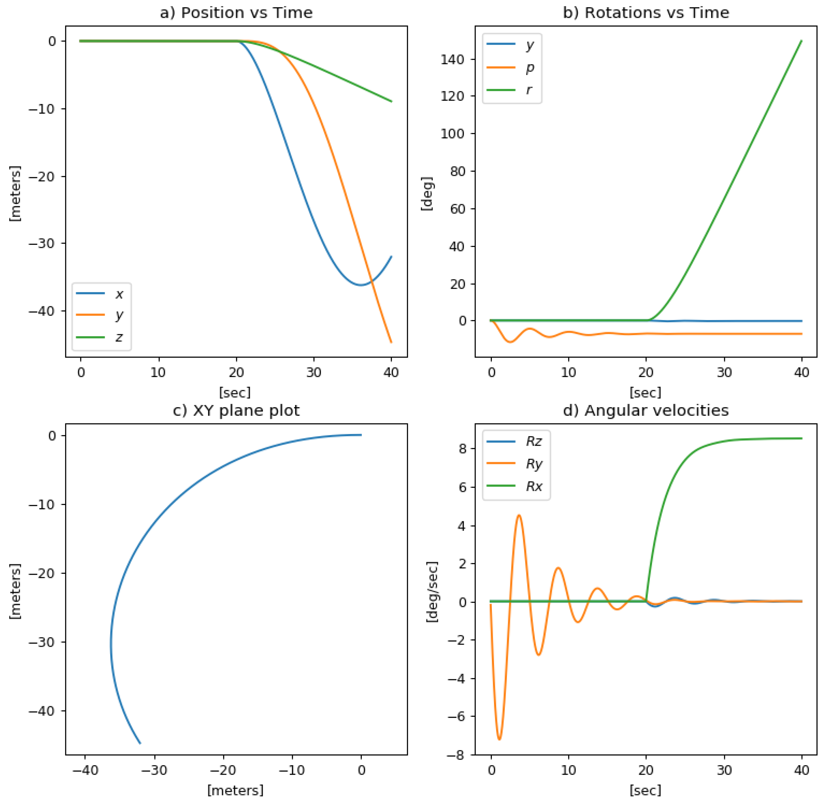
To test the simulation we generate a demo scenario. We put the ROV underwater without applying any external thruster force for 20 s. In terms of the simulation this means that the initial integration conditions of the generalized speeds and coordinates are set to zero. The next 20 s hence the second stage. We apply an uneven thrust force for thrusters 1 and 2 (described in Figure 2).
In Figure 3, we can see that in the first stage since the ROV is positioned with 0 pitch angle and, since the COB point is not directly above the COM point, the ROV is oscillating around the y axis. The oscillation are dampened due to the dampening drag forces described in the previous subsections. In the next stage we can see that the ROV is turning due to the uneven thrust forces applied. The ROV is also in a dive since it was stabilized in a negative pitch as can be seen in Figure 3b.

3.2. Conclusions

We have presented a step by step procedure for creating a dynamic rigid body underwater ROV simulation. The output of this process is formulated in Equation (16). This form of representation decouples the model developed from the actual simulation. This means that we can use the output (“Mass matrix” and “Forcing vector”) and integrate it into any simulation framework independent of programming language or operating system. In addition, this method is highly configurable. For example, We can easily add an additional thruster and position it in the ROV frame. We can test the new configuration in different scenarios as demonstrated in the previous results. We presented the process of integrating the simulation products in the final full-scale 3D simulation. Some assumptions we made in order to simplify the simulation. For example, we ignore Coriolis forces due to the low relative speeds in which underwater ROVs are moving, having said that modifying the simulation in that vector is achievable.

4. Tether Simulation

The previous section was dealt with the dynamics of the ROV and was simulated using a force based method from the mechanical engineering domain. Simulation of dynamic systems in computer graphics mainly use force-based methods, where linear and rotational accelerations are computed from forces and torques. A time integration method is then used to update the velocities and positions of the object as shown in the previous section. In contrast, geometry-based methods work directly on vertex positions, modifying them using iterative update equations. The main advantage of a position-based approach is its controllability. In force-based systems, overshooting problems associated with explicit integration schemes can be avoided. In addition, collision constraints can be handled easily and penetrations can be resolved completely by moving points to valid locations [19].
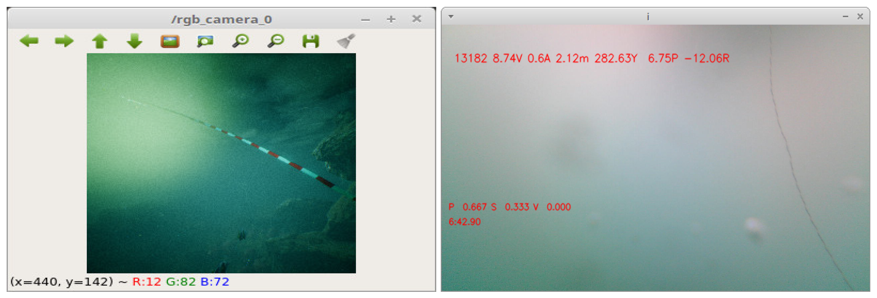
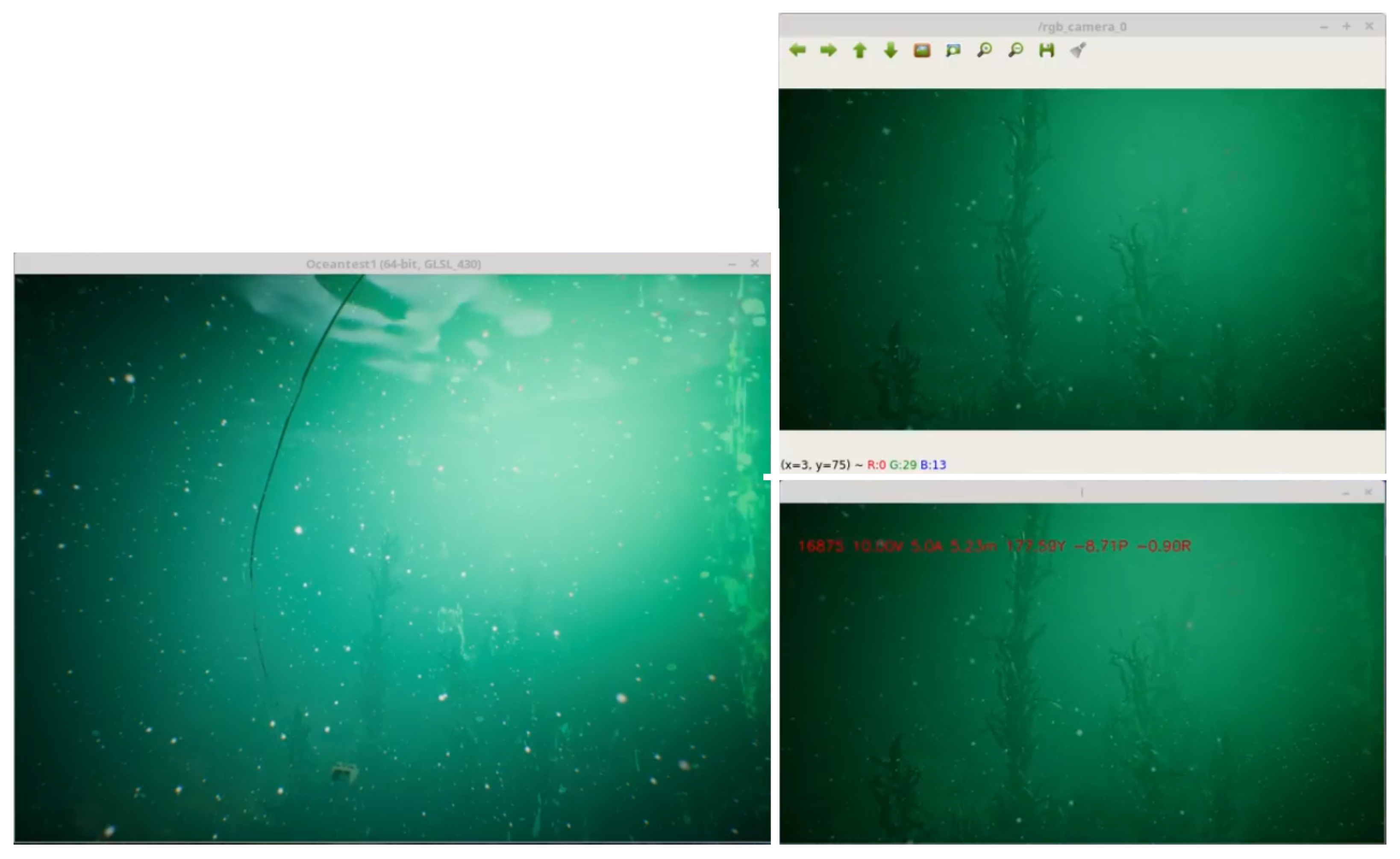
In our research, we found the tether simulation to be particularly useful in cases were the robot sees its own cable as presented in Figure 4. This fact may disrupt computer vision algorithms—especially those based on tracking using landmark features from the images and assume that these landmarks are not moving in the scene. With this type of simulation, that kind of behaviour can be simulated in a manner close to real cable behaviour. New computer vision algorithms can be developed to mitigate that behaviour and new control algorithms can be developed to manage the cable configuration.
The position based simulations which were originally developed for the simulation of solids were also extended to the area of fluid dynamics [20] where it is not reasonable to simulate the interacting forces between the particles in real-time. In contrast to force based simulation, position based models can scale up and can be used today to simulate large multi-body systems such as fabric or fur in real-time. While force based systems tend to be physically accurate under certain assumptions, position based systems aim to be visually realistic. For example, a set of simulation parameters may not correspond to real physical values, but may generate realistic object behaviour as the output. The stiffness parameter implemented in the Unreal Engine, which we will later discuss, is an example of a parameter that influences the dynamic behaviour of the position based cable model but has no meaningful physical value (such as mass or length).
Our tether cable simulation method, in terms of number of particles, lies between the forced based system and the position based system. In simulating a long cable with a large number of segments, we aim for real time performance by applying constraints and also use position based models. In our underwater cable implementation, we take the existing Verlet integration suggested by Jackobson [21] and modify it to simulate a realistic underwater cable.
The existing rope simulation in Unreal Engine 4 platform, which we will discuss later, performs in a convincing way only in a light density environment like air but looked quite non-realistic in the aquatic medium. This motivated us to return to the original assumptions of the simulated implementation and modify it in order to create visually convincing underwater rope/cable simulation. In our work, we added extensive damping and random displacements to the particles and experimentally analysed and verified the resulting behaviour. Specifically, we were interested in the behaviour of variable length long cables attached to the ROV at one end and to a spool in the other end.That kind of cables have some unique physical characteristics that could not be addressed by the current features in existing simulation frameworks.
Most of the underwater cable modelling was done in the mechanical engineering domain using force based methods. Cable and chain models in general are simulated using a segment based model [22]. On the other hand position based methods are used widely in the computer graphics domain. Jackobson [21] described in detail the position based model for cable simulation. His work was the basis for the current implementation in today’s game engines [23]. Our work is based on the survey paper by Bender [19] on different position based methods currently used in computer graphics. In this section, we will describe in detail the theory of position based methods with focus on cable simulation in addition to our model. We will also demonstrate and analyse a 2D simulation of our model.

4.1. Algorithm Overview

The Unreal game engine uses the Verlet integration method for rigid multibody simulation presented by Varlet [24]. The heart of the existing rope simulation is a particle system. Each particle has two main variables: Its position x and its velocity v. The new position x t + Δ t and velocity v t + Δ t are computed by applying the rules:
x t + Δ t = x t + v t Δ t
v t + Δ t = v t + a t Δ t
where Δ t is the time step and a t is the acceleration. For obtaining a velocity-less representation of the above scheme, instead of storing each particle’s position and velocity, we store its current position x and its previous position x t Δ t . Keeping the time step Δ t fixed, the update rule (or integration step) is then:
x t + Δ t = 2 x t x t Δ t + a t Δ t 2
x t Δ t = x t
x t = x t + Δ t
Jackobson [21] suggested in his paper that by changing the update rule to x t + Δ t = 1.99 x t 0.99 x t Δ t + a Δ t 2 , a small amount of drag can also be introduced to the system. This is a useful equation that can be further modified to add large drag or damping to a system in an aquatic environment. In our implementation, we added small random displacements for creating micro current effects suitable for ocean-like environment. Those micro currents prevent the rope from looking frozen in space where there are no other forces presented to the simulation. This is usually the case in long low tension cable characterized by tethered systems. Our proposed final model can be summarized by the following equations:
x t + Δ t = x t + ( x t x t Δ t ) D r + a Δ t 2 + ϵ r
x t Δ t = x t
x t = x t + Δ t
where D r is the drag coefficient with maximal value of 1 (no drag). It is set to 0.9 to introduce a large amount of drag typical of aquatic systems and is multiplied by the velocity term ( x t x t Δ t ) . When the time step Δ t is set equal to 1 for simulation purposes. ϵ r is the added random displacements to simulate random forces generated by underwater micro-currents. ϵ r was uniformly distributed and limits were chosen to be small enough so the random behaviour will only cause long-term effect on the cable.
The next step of the rope simulation is to apply the distance constraint. This means that the distance between adjacent particles should be kept constant. This process is done iteratively by pushing the particles directly away from each other or by pulling them closer to maintain the required distance. The following pseudo-code (Listing 1) describes this process:
Listing 1. Distance constraint algorithm.
SolveDistanceConstraint(PosA,PosB,TargetDistance):
  Delta = PosB-PosA
  ErrorFactor=(|Delta| - TargetDistance)/
        |Delta|
  PosA += ErrorFactor/2 ∗ Delta
  PosB -= ErrorFactor/2 ∗ Delta
 
SolveConstraints():
  for iter=0 to SolverIterations
    for ParticleIndex=0 to NumOfParticles-1
   SolveDistanceConstraint(
     Particles[i],Particle[i+1],TargetDistance)
    for ParticleIndex=0 to NumOfParticles-2
      SolveDistanceConstraint(
        Particles[i],Particle[i+2],2∗TargetDistance)
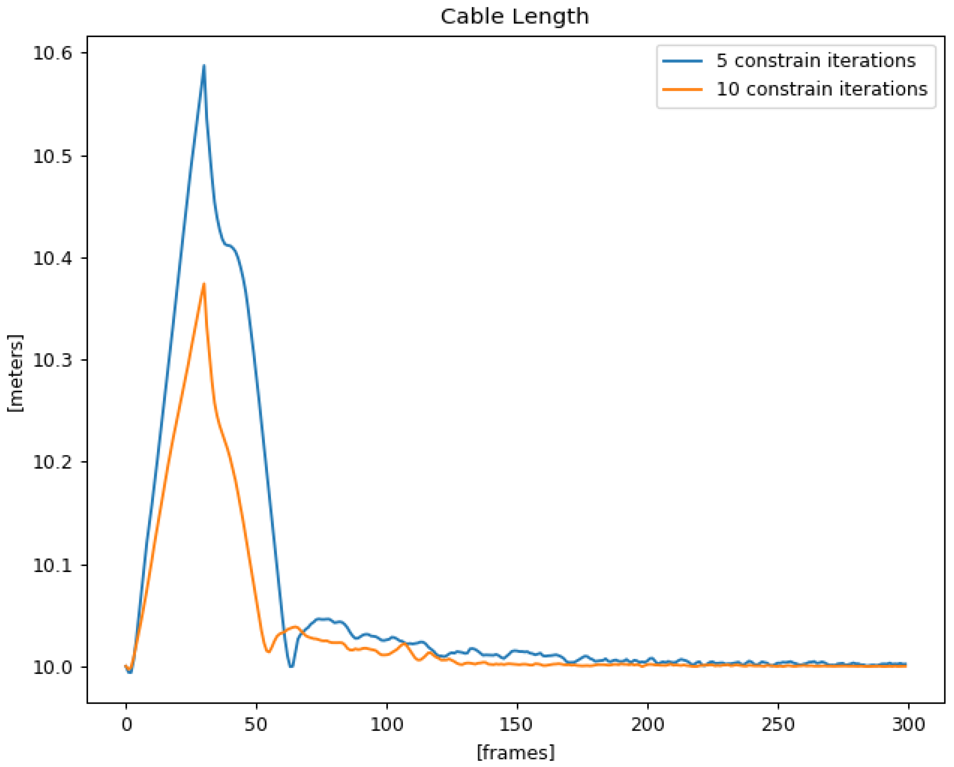
This pseudo-code above shows how distant constraints are implemented in Unreal Engine 4. We can see that the “SolveConstraints” function has one outer loop which is responsible to perform iterations to enforce the constraint. More solver iterations will give more stiffness to the cable. In Figure 5, the length of the rope is changed when introducing a force at one of its ends and changes in the overall length is dependent on the number of constraints and iterations applied to the rope particles. The second inner loop reduces the flexibility of the rope by enforcing constraints between particles that are separated by one other particle. That specific constraint limits the ability of the rope to bend. Figure 6 shows the difference between the two constraints. The bending constraints were useful in smoothening out the effects of random displacements added to the underwater simulation. Finally, our final solution was implemented as a new underwater rope plugin.
The rest of the changes to the rope characteristics were made by parameter changes to the model. Cable length was chosen to be 10 m and the number of segments was chosen to be 100. This was done in order to create a large amount of short segments, required for visually realistic underwater simulation. With such models, any disturbance at one end of the cable will propagate slowly and will be damped by the surrounding water body.
The SolverIterations parameter (as can be seen in the pseudo code) should be chosen carefully. There is a trade-off between the stiffness or the ability to stretch and the damping mechanism introduced earlier. Since the damping is done in the Verlet stage, the constraint mechanism can still freely move all the rope particles, and due to that trade-off we limited the number of iterations. An improvement can be made to add some damping effect also in the constraint stage. That will allow more control on the cable length.
Setting the gravity to be zero was done to simulate the effect of neutral buoyancy. Usually, tethered systems are designed to meet the goal of neutral buoyancy to eliminate pulling forces from the cable in the case of non-neutral buoyancy. Additionally, the negative buoyancy of a tethered system can cause the cable to be tangled with objects on the surface of the seafloor.
Drag coefficient was chosen to be 0.9 and this value is much lower than the maximal value 1. This was done to introduce intense damping and to reduce the propagation along the cable. The random displacements coefficient was chosen empirically to be 0.1 and can be adjusted to different sea conditions. All the parameters of the simulation included the added parameters (the damping and the random displacements) can be controlled by the outside environment (like the game engine editor) and can be adapted to different types of cables with different characteristics.
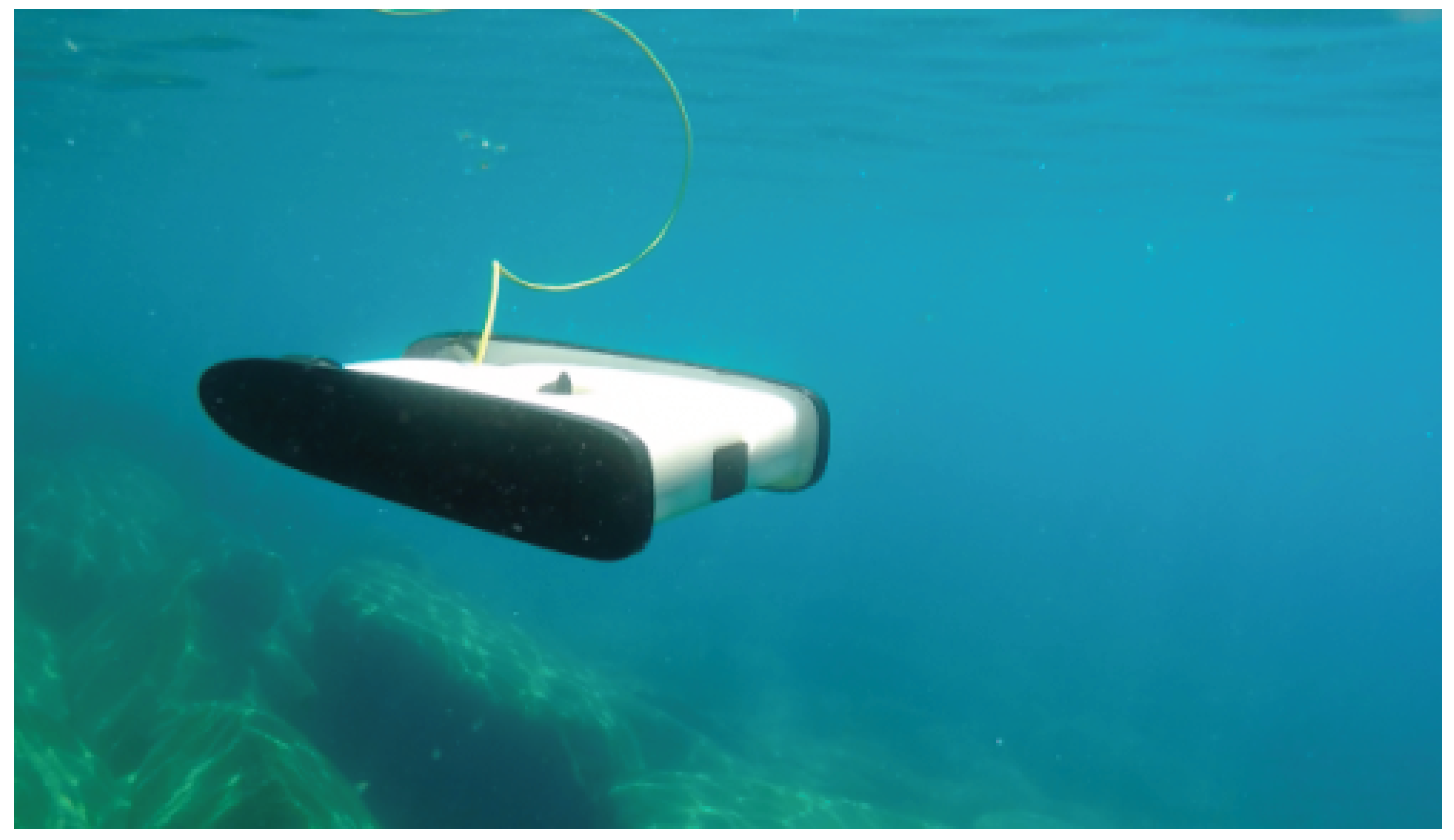
In our tethered ROV simulation, we have also made additional assumptions that there are no forces or relatively small forces introduced by the rope which effect the ROV position. In some cases, it makes sense for example if the mass of the ROV is relatively much higher then the mass of the rope. For example, the OpenROV (Figure 7) [25] robot uses a very thin cable which handles only communication (not power) and in this case, we can assume that unless the cable is fully extended the relative force applied by the cable is relatively small. In practice, This means that the rope is not limiting the ROV movement.

4.2. Variable Length Cables

Underwater simulation of ROVs will also require modelling of cables connected to a spool that are released or retracted according to a naive logic that whenever there is a tension in the cable the cable is released. In the following, we outline a method to extend our model to a generate a variable length cable.
A flag is associated with each vertex of the cable model, and it represents whether the vertex is free to move according to the Verlet integration and the constraint mechanisms. By default, both ends of a cable will be flagged as non-free and the rest are free, since the cable is attached to both ends. In the case of a spooled cable, all the particles of the rope that are currently not released are flagged as non-free particles.
Since our model is position based, whenever the first segment from the spool side is stretched enough, typically by 10 percent of the total length, we will release a particle/vertex. After that, the Verlet integration and the constraint mechanism will move into action and will adjust the particles accordingly.
We have made further modifications in the model, particularly in the areas closer to end points. Random forces were not be applied on the first free segment, to avoid the spontaneous release of the cable due to random change of the length of the first free segment.
The spooled cable extension is done with the intention to lay a simulated foundation for the development and testing of managed tethered system. The simulation can report in real-time the current length of the cable and the estimated tension of the cable at each point along the cable. Specifically, in the beginning and the end of the cable wherein a real system we can place tension sensors as an input to the controller of the tethered system. The tension can be measured as a function of the distance between every two particles.

4.3. Methods and Tools

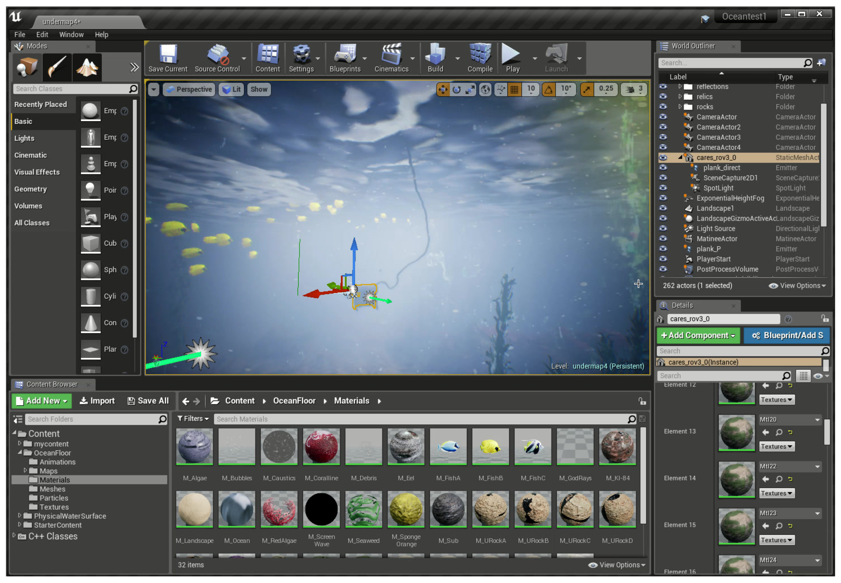
The main aim of this work has been to generate a convincing and realistic behaviour of an underwater tethered robot using the simulation framework provided by the Unreal Engine 4 (Figure 8). A live video demo can be seen in videos [26,27] and a snapshot is given in Figure 9. The experiments were done in the editor environment (not as a packed game). The robot seen in those figures was moved manually while the cable was attached to both ends. The new plugin is maintained and can be downloaded from here [28].
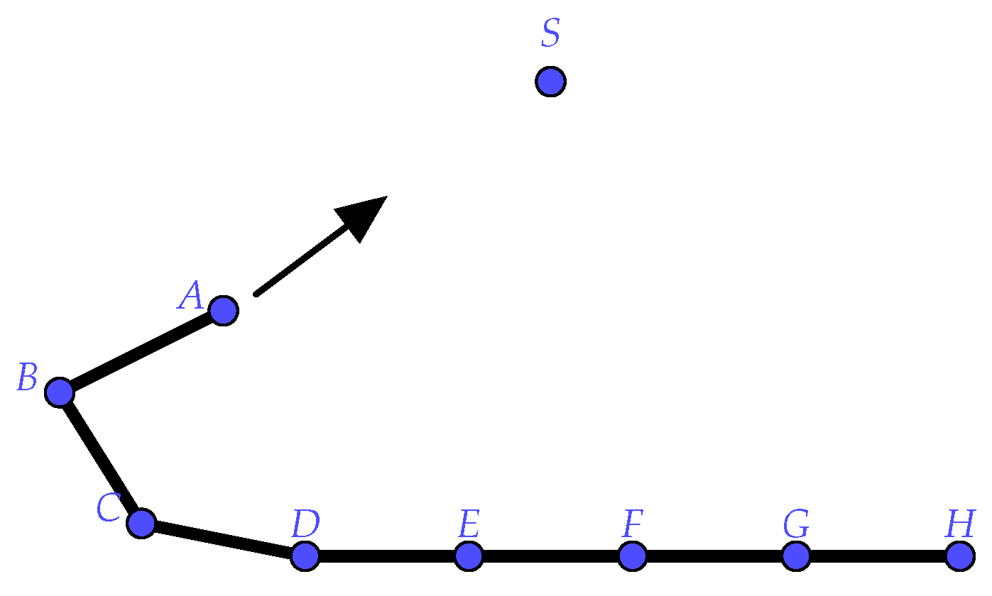
In addition, to have finer control over the simulation, an additional 2D simulation was created to demonstrate the proposed method. We used the Jupyter [29] python notebook environment to generate the output seen in Figures 11–13. The 2D simulation is maintained under the following link [30]. Figure 10 illustrates the cable configuration used in the 2D simulation.

4.4. Experimental Results

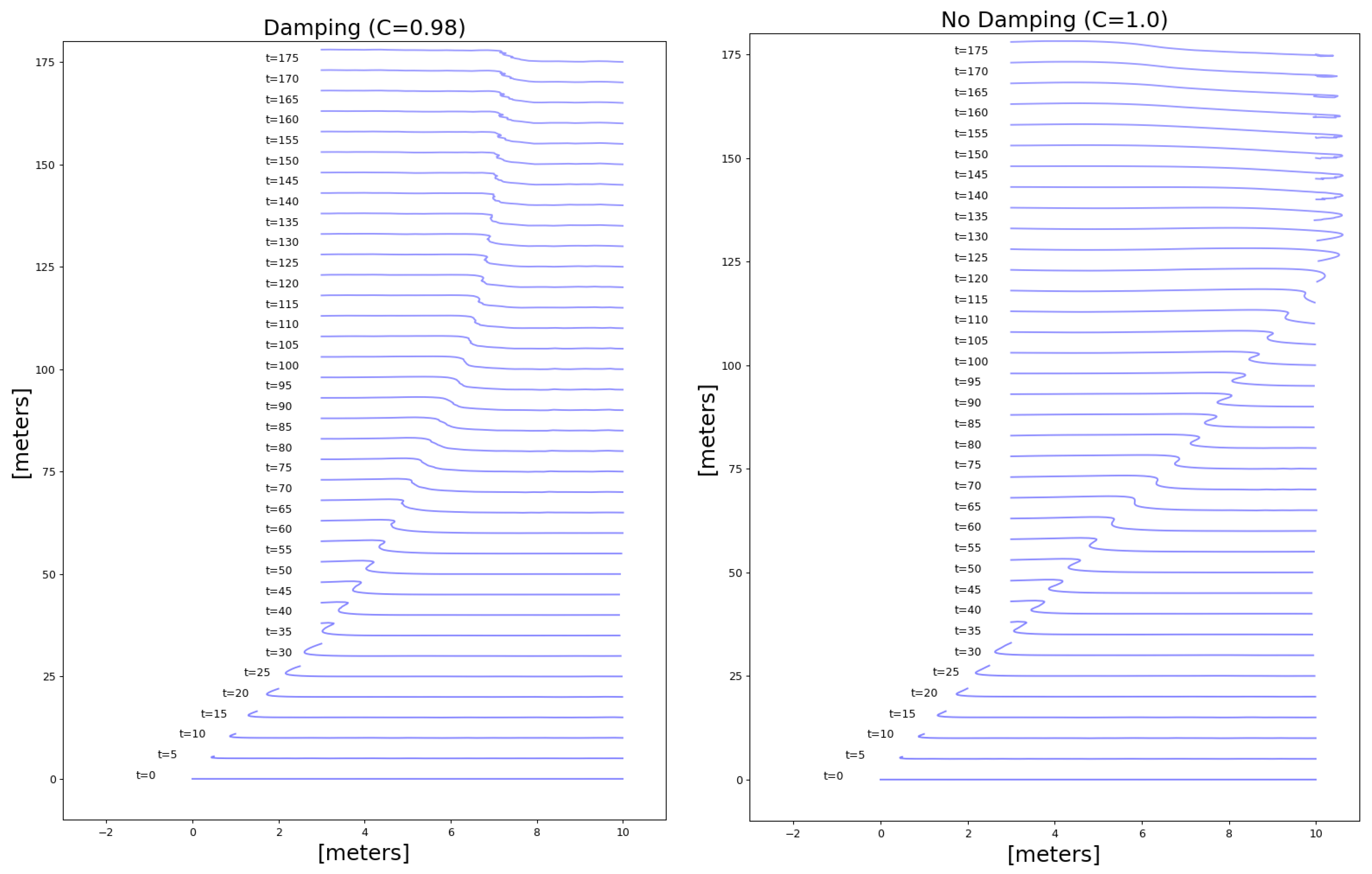
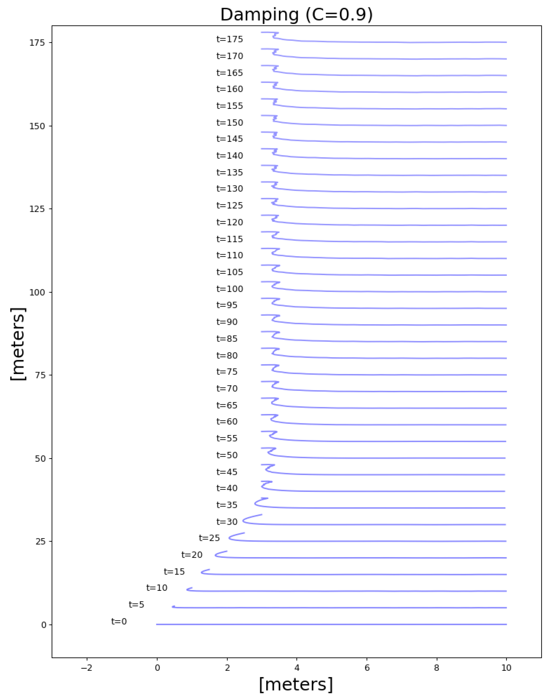
We created a simple 2D computer simulation to simulate the effects of moving one edge of the cable while the other end is pinned (Figure 9). Figure 11 shows the behaviour of the rope with and without damping with respect to time. The wave motion continues to propagate through the rope when there is no damping whereas with damping the wave energy slowly decays and random forces are becoming more dominant. In Figure 12 we can see our desired effect when using coefficient 0.9. The movement of the cable at one end does not affect the other end, so long as there is no tension in the cable segments.
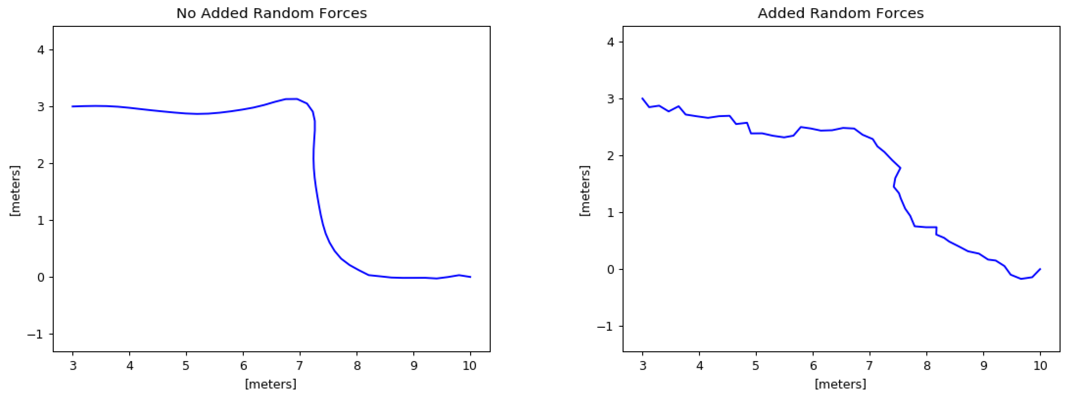
Figure 13 shows the random forces effect. In this experiment we look at the cable configuration in the 2D space after the system is stabilized ( t > > 0 ) with and without random forces. We can see that the random forces create a kind of memory loss effect of the shape of the cable. This effect is important when there are no other significant forces (or they are close to zero) in the system. When we don’t add the random force, the cable tends to stand still in contrast to what would be expected in a dynamic aquatic environment.

4.5. Conclusions

In terms of performance, the modifications to the current model didn’t require more computational effort. In fact, if we assume neutral buoyancy of the cable we can remove the gravitational forces from the simulation to reduce computational time. This can be useful in cases where a large number of cable/rope-like object are simulated. Generally speaking, we can say that a cable is a linear 3D object curve which can be efficiently computed by modern CPUs. Using the position based approach allowed us to easily modify the current model by adding drag and random displacements and in the future to apply other constraints for inter-rope tangling and ROV interactions. Currently, we are not dealing with the forces applied to and by the cable to the objects that it is connected to. Further improvements to this model can be done by measuring the length of the segments as described in Section 4.2 and translate this length to a tension applied to the ROV as an outside torque or force. In our current implementation, we assume that there are no forces and torques applied by the rope which effect the ROV movement.

5. The Underwater Ocean Environment

Simulating visually realistic marine environment can be challenging due to the presence of several factors affecting the illumination and motion of objects within a region. In contrast to the air medium, the underwater marine environment appears significantly more turbid and dynamic, being rich with organisms. Each organism has its own special visual characteristics and dynamics. They can be for example, semi-transparent like jellyfish or completely opaque. The scene can be highly dynamic where schools of fish pass very close to the camera. Such complex and dynamic environments need to be modelled for simulating the motion of an underwater remotely operated vehicle (ROV). This section focuses on generating the underwater ocean environment and the generation of bioluminescent plankton in the marine environment and the associated visual effects. Today the visual capabilities of game engines are exceptional. Those capabilities are motivated by a multi-billion industry and the rapid advancements in the graphics hardware domain. In our simulation which focuses on the realism of the environment, using game engine is a natural choice.
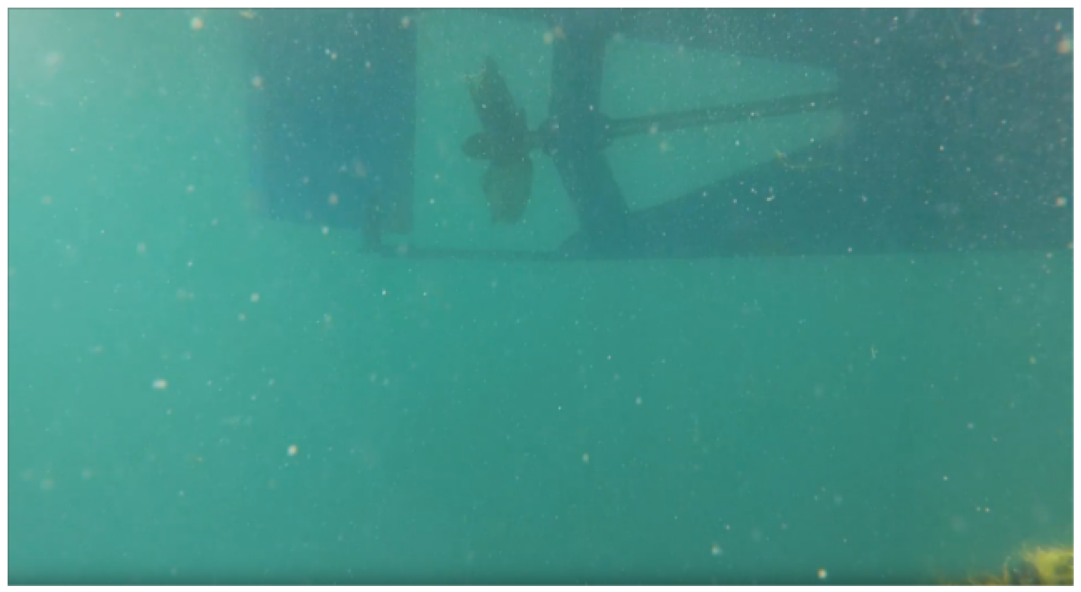
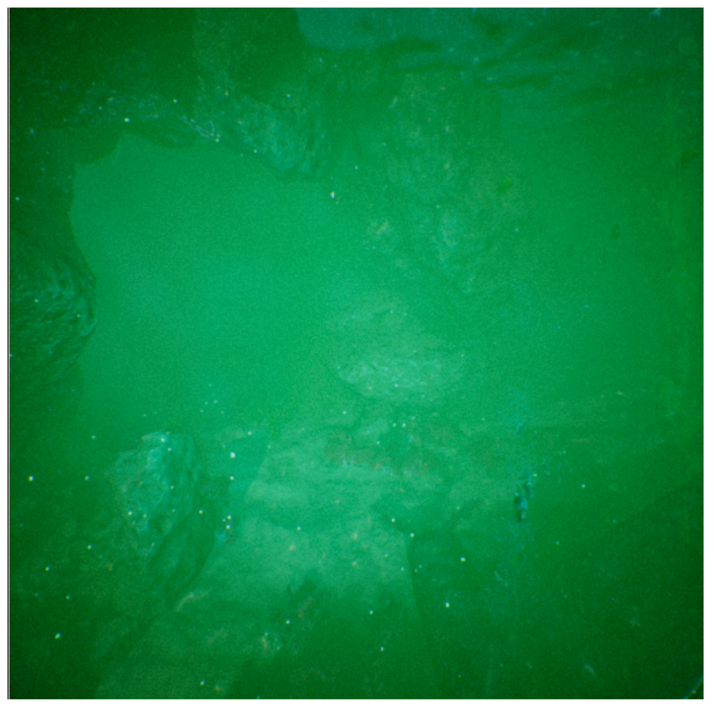
Figure 14 presents an image we took underwater in an area rich with organic matter. The predominant fog and snow like particle effects are created by plankton. This figure clearly shows the need for realistic plankton simulation both for testing computer vision algorithms and also for human training purposes. Although some visually simulated underwater environments exists in game engines, to the authors knowledge, no prior research work has been reported on graphical modelling and simulation of plankton. In this section we’ll give some background information regarding relevant marine environment characteristics, we’ll give an example of existing simulated underwater environment in Unreal Engine and we’ll discuss in detail about the two types of plankton (zooplankton and phytoplankton) which we modelled in order to create a more convincingly underwater ocean behaviour.
The marine environment supports two basic types of marine organisms. One type comprises of planktons or those organisms whose powers of locomotion are such that they are incapable of making their way against a current and thus are passively transported by currents in the sea. The word plankton comes from the Greek planktons, meaning that which is passively drifting or wandering. Depending upon whether a planktonic organism is a plant or animal, a distinction is made between phytoplankton and zooplankton. Although many planktonic species are of microscopic dimensions, the term is not synonymous with small size as some of the zooplankton include jellyfish of several meters in diameter. Nor are all plankton completely passive; most, including many of the phytoplankton, are capable of swimming. The remaining inhabitants of the pelagic environment form the nekton. These are free-swimming animals that, in contrast to plankton, are strong enough to swim against currents and are therefore independent of water movements. The category of nekton includes fish, squid, and marine mammals [31]. In addition, the marine environment also include plants like seaweed and also some natural static objects such as rocks. Man-made objects are also significant part of the sea in the form of boats structures and also (unfortunately) garbage.
From an optical imaging point of view, seawater is an absorbing and scattering medium. Light energy that propagates in water is absorbed by water molecules and dissolved organic matter (DOM) or suspended sediments [32]. Propagating light is also elastically scattered by thermal fluctuations in water (Rayleigh scattering) and by hydrosol particles suspended in water. The major portion of absorbed energy is transformed into heat. The rest of the absorbed energy is re-emitted as Raman scattering and fluorescence. Elastic scattering occurs without a change in energy only the direction of propagation changes [33].
Underwater optical imaging systems can be broadly classified into two areas: passive and active. Passive systems utilize light in order to image objects that have been illuminated by some source other than that associated with the imaging system. Examples are imaging of objects using sunlight or other sources of illumination such as bioluminescence. Active systems take advantage of a user generated source of light. A simple example is an underwater camera system which uses either strobe or continuous artificial illumination [34]. In both systems (active and passive) backscattering or diffuse reflection (reflection of light waves back to the direction from which they came) is another effect that is commonly seen as shown in Figure 14. In the active system, we can control the intensity of backscatter by reducing the intensity of the light or changing the position of the strobe relative to the camera, whereas in a passive system we need to change the camera orientation or use special filters.
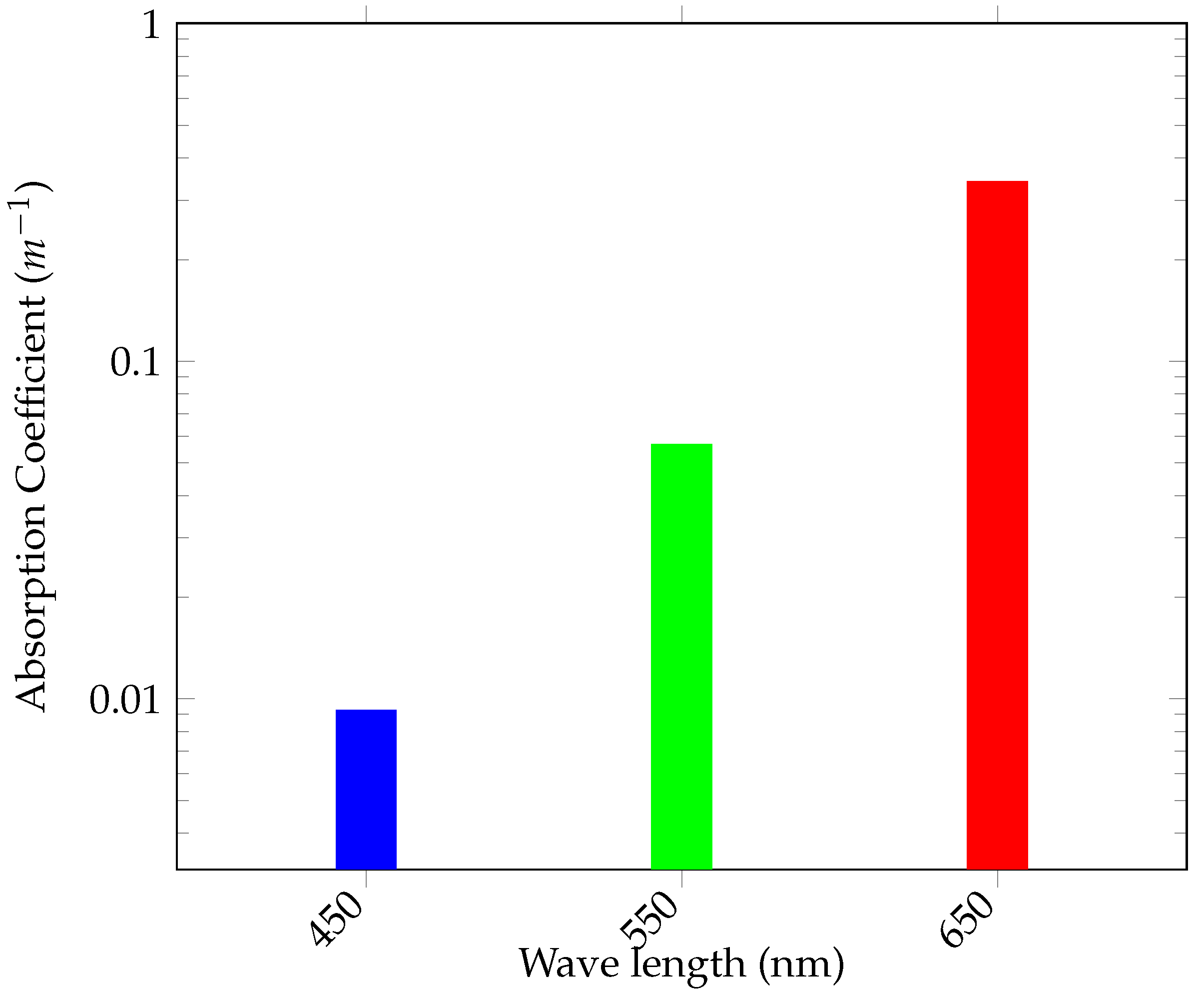
Colour propagation underwater is yet another important aspect we need to consider in our simulation. In Figure 15, the absorption coefficients of fresh water at different wavelengths are shown on a logarithmic scale. The ratio between the red spectrum (approximately 650 nm) and the blue spectrum (approximately 450 nm) is almost 40 which means that the red part of the spectrum will be attenuated rapidly and after a short distance it won’t be visible whether the white light comes from the sun or from a strobe. The green light will propagate a little further until only the blue light is seen. This is why in order to get colourful results ocean photographers try to get as close as they can to the object of interest.
Intrinsic characteristics such as the camera hardware plays an important part in the effects we see. Motion blur caused by camera movement is common in underwater systems. The long exposure times that are used to compensate for the lack of underwater lighting is responsible for that effect. We will discuss this effect in the following sections.
There are some additional optical and underwater imagery effects such as the chromatic aberration [37], which is caused by a relatively wider field of view. Those effects which are supported by modern game engines and can be easily added to the simulation [38].

5.1. Generating Marine Environment in a Game Engine

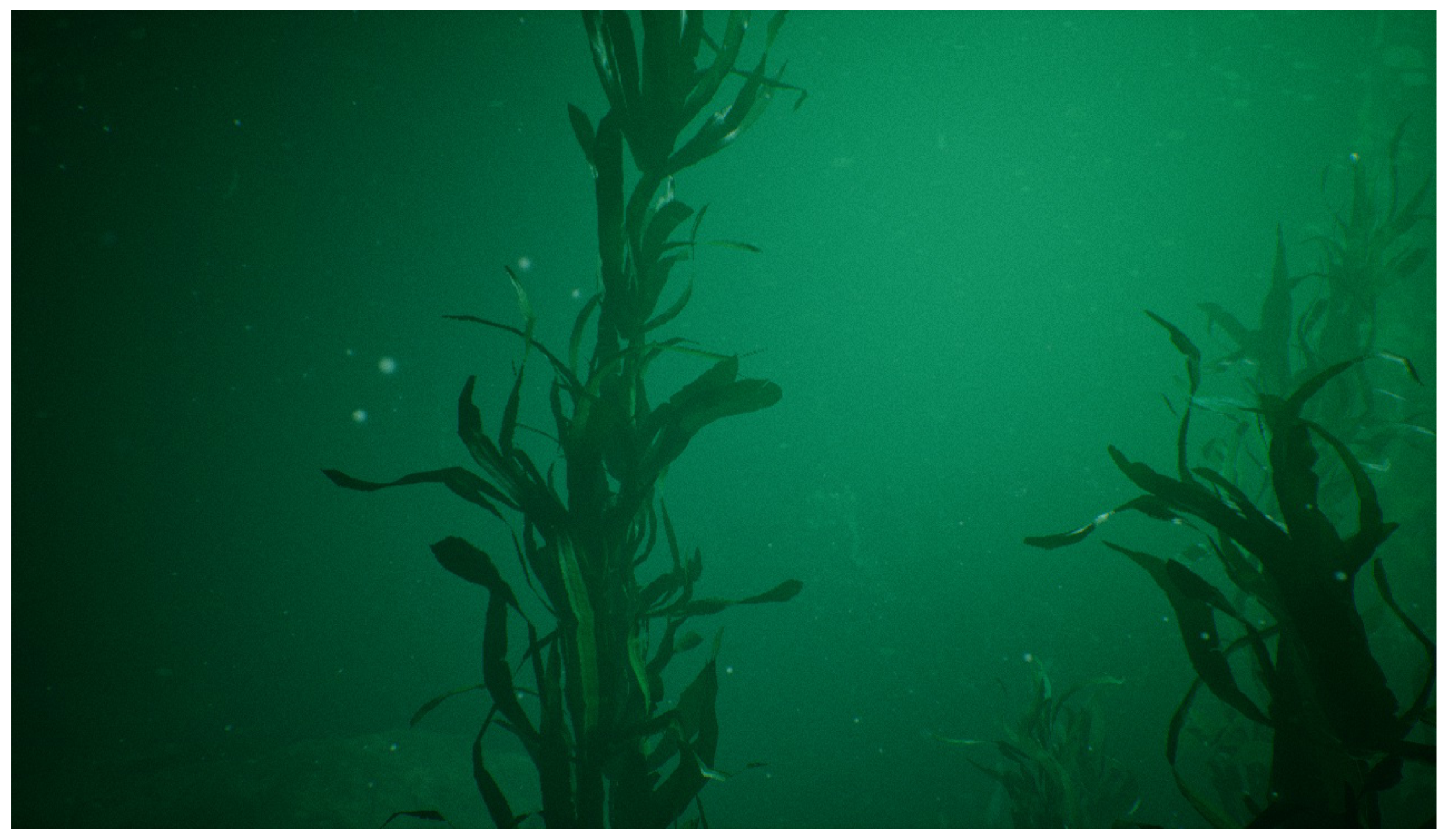
From a research perspective, working with a game engine as the provider of the visual world is similar to finding or creating a real-world scene for the purpose of doing an experiment. For example, going outside and finding a suitable place for an outdoor experiment is parallel to the process of searching an existing environment in a game engine marketplace. In a Game Engine marketplace, we can find an existing environment that we can manipulate for our purposes. This process needs to be done carefully since environments taken from a marketplace engine might have some unreal effects for gaming and entertainment purposes. In our case, we took an existing underwater marine environment with existing rocks, fish, relics etc. [39]. Figure 9 shows such a rich environment. We can see in this image some rocky structure such as an underwater rock gate, some fish and also our simulated robot manoeuvring. For a more complete visual simulation we added to it some other needed components such as the ocean plankton which we will discuss thoroughly in the following sections. The end result (as can be seen in the attached videos) was that we got was a convincingly realistic underwater environment which we could control and manipulate as needed. We can control and move any object in the scene and for some objects we can change some key characteristics to simulate different conditions. Figure 16 shows a seaweed simulation taken from the package [39]. The seaweed which has a root planted on the sea floor is free to move according to the ocean currents. The seaweed component simulation is based on the unreal engine SimpleGrassWind which when applied underwater gives similar effect [40]. We can control the amount of wind and type by changing the relevant blueprint.

5.2. Simulating The Camera

The intrinsic parameters of the camera have a large impact on the behaviour and performance of a computer vision system. For the purpose of simulating the camera, we are using the SceneCapture2D component which is used for the purpose of rendering the scene into textures. Game engines use this component to simulate scenes with a screen like objects like security cameras and monitors for example. In this subsection, we are covering the main adjustments we made to the physically based camera model of the Unreal Engine SceneCapture2D component to the underwater environment.
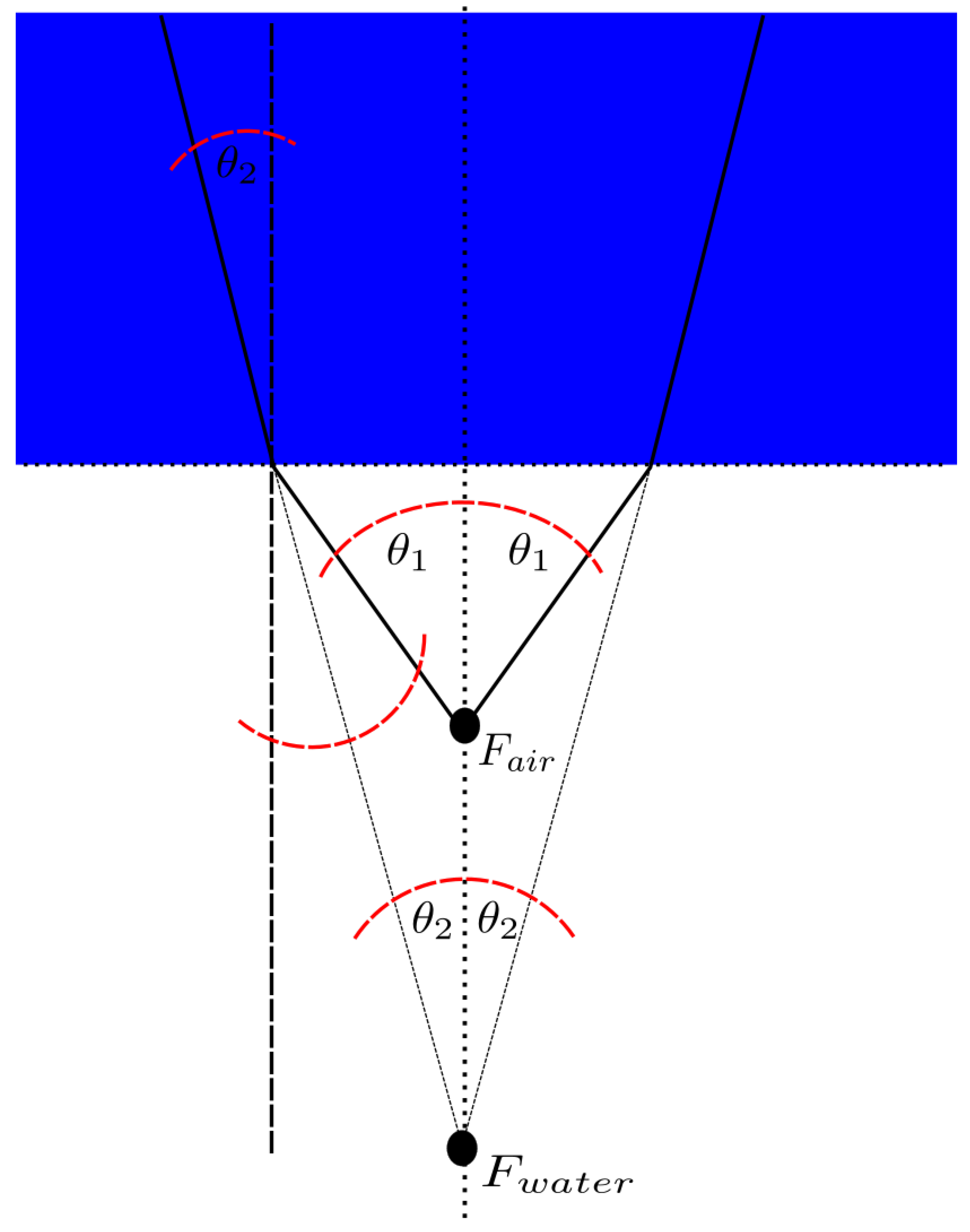
The first was the field of view. Since we are modelling underwater vision conditions we need to update the camera model underwater. For simplicity, we assume a perfect pinhole camera model without distortion. As an input to the game engine, we need to choose the horizontal field of view (FOV). From Snell’s law we know that:
sin θ 2 sin θ 1 = n 1 n 2
where each θ is the angle measured from the normal perpendicular to the boundary and n is the refractive index of the respective medium. In our case our ray of light is moving through water and then to air (we ignore the effects of the port) and we get magnification of 1.333. From Equation (25) we can calculate the effective FOV underwater as described in Figure 17 and summarized in Equation (26).
F O V w a t e r = 2 arcsin ( n 1 n 2 sin ( F O V a i r / 2 ) )
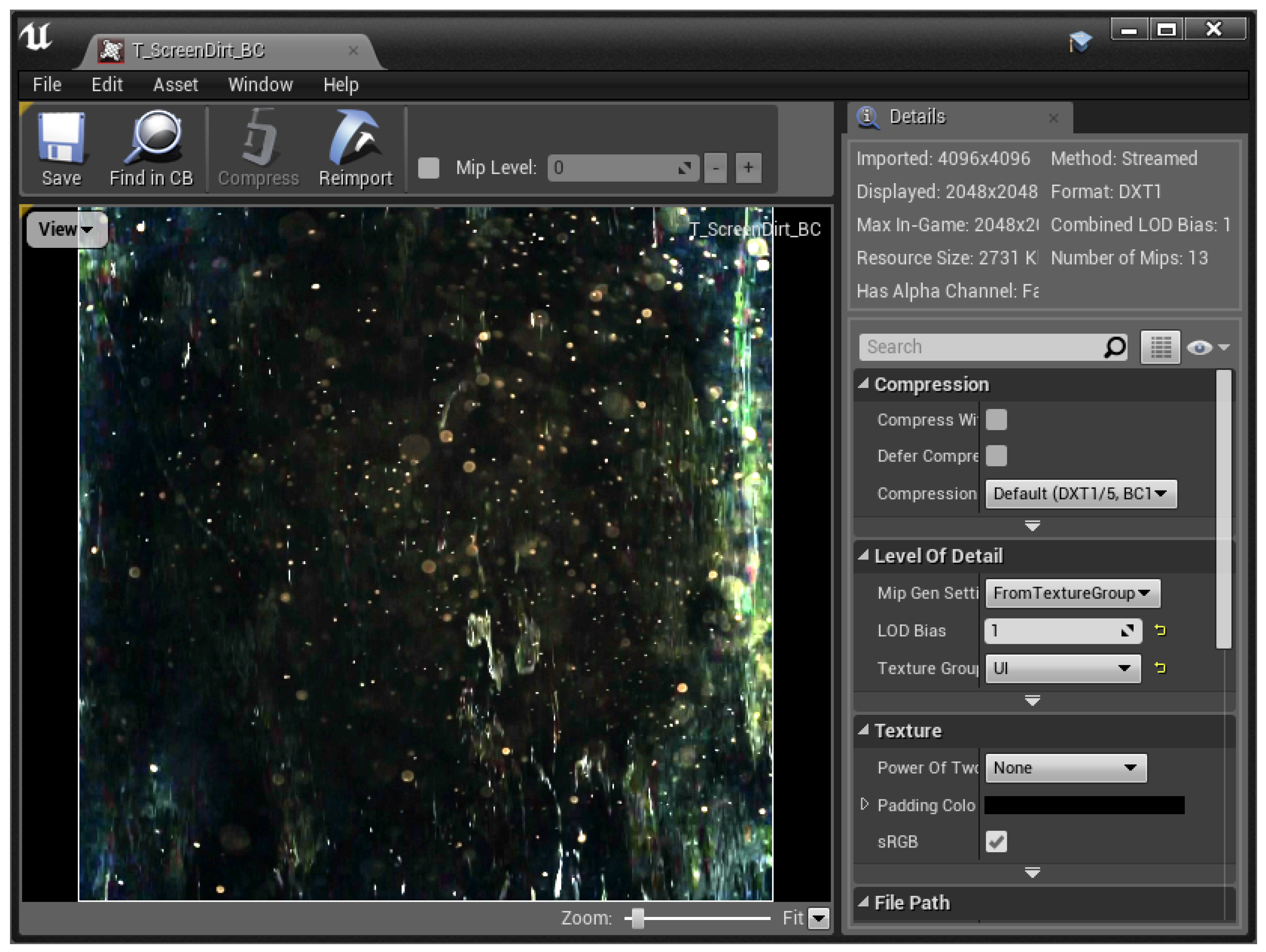
The Unreal Engine uses physically based post process effects which we can use to better represent the under water conditions. One aspect was the adding of a dirt mask on top of the camera lens. It is quite common in an underwater environment to have dirt accumulated on the port edge facing the water. This effect depending on the magnitude of the accumulation can be significant and may affect computer vision algorithms such as tracking. Figure 18 shows a dirt mask pattern (From [39]) we applied in Unreal Engine on our camera component. The dirt mask is blended with parameterized intensity to the camera image.
For additional image noise we added grain noise filter which is also common under low light conditions. Adjusting the grain filter can be done directly in the game engine and we can control the jittering and the intensity.
Another post process effect is the chromatic aberration that simulates the colour shifts in real-world camera lenses. The effect is most noticeable near the edges of the image and in relative large FOV angles lenses. The magnitude of the effect is parameterised and experiment can be made to explore the different effects of different values on computer vision algorithms.
We can also simulate the depth of field. Unreal Engine supports cinematic methods and it is aligned with common camera options. In our underwater simulation we didn’t focus on that effect (in terms of testing) since the outcome of this effect has some overlap with the fog effect which was more significant in our simulation.

5.3. Simulating Plankton

The movement of plankton is dependent on ocean currents and currents created by moving object like fish movement or even robotic arm movement can shift the water from side to side which in turn will create a visible movement of plankton. We ignore the hydrodynamics affects that plankton might have on an ROV, we assume that the water are relatively clear and the main mass is pure water. The visual effects of the plankton on the other hand is significant as can be seen in the real image Figure 14.
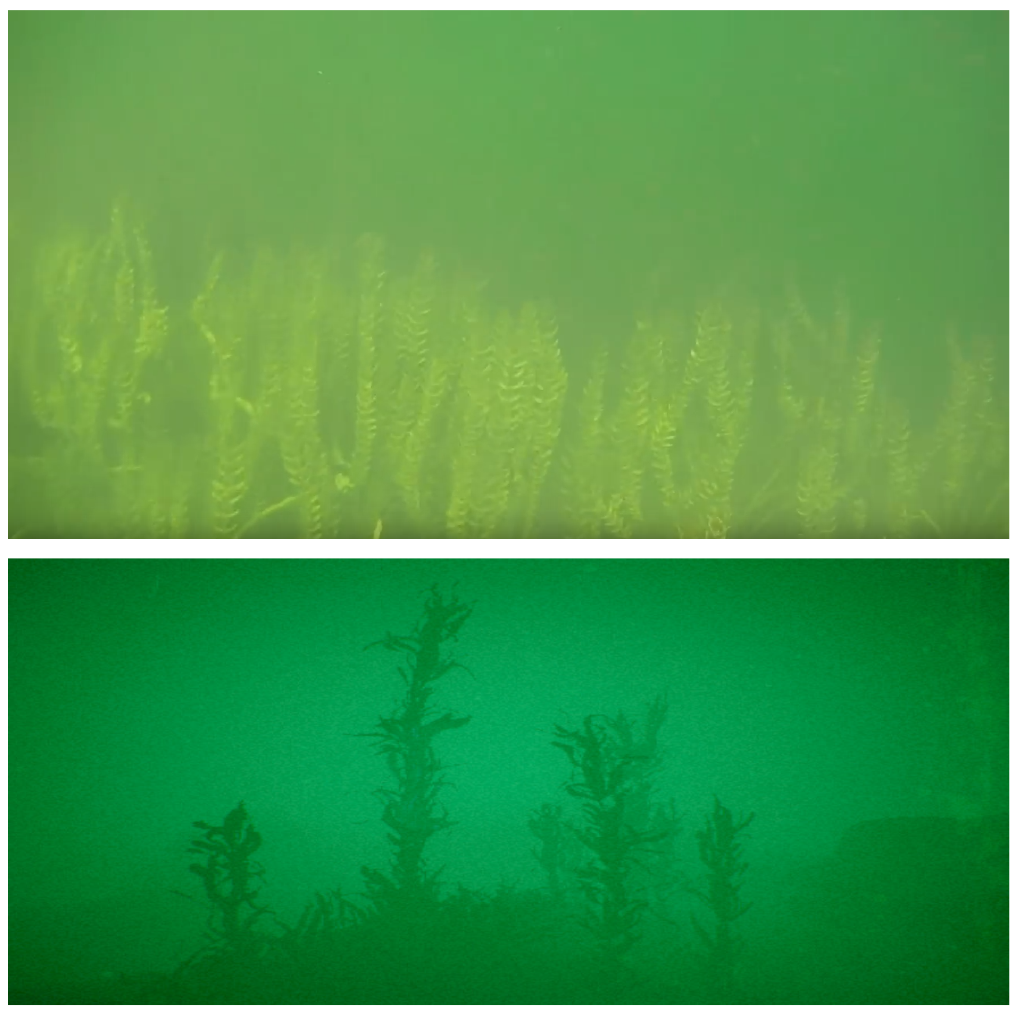
Phytoplankton are microscopic photosynthesising organisms. Therefore they are not visible directly to the naked eye. Due to the chlorophyll content in their cells, the green pigment is sometimes noticeable. We can find them in the upper layer of a large body of water exposed to sunlight. Interestingly enough, their optical properties can be simulated using Exponential Height Fog [41]. Exponential Height Fog creates more fog density in low places of a scene and less density in other places. Exponential Height Fog provides two fog colours which are used to differentiate upper and lower layers of the atmosphere. We can use this effect to our advantage by choosing a green colour for the surface level of the sea and the blue colour to deeper layers. The transition between the colours is smooth. Figure 19 shows the final result of simulating only Phytoplankton using the Fog component in Unreal Engine. We present two images for comparison: one is a simulated output and the other is a real image taken underwater.
To simulate zooplankton, which are larger and more visible particles, we used the Unreal Engine 4 particle engine [43]. In general, particle systems or engines consist of several important parts. First is the emitter which is responsible for releasing the particles. We can also control the shape of the emitter and the direction the particles are distributed. Secondly, particle dynamics specify the way the particles move through space. The particles may be randomly distributed, move along a curvilinear path, move under the influence of forces or combinations of the above. Thirdly, physical characteristics of the particles define the shapes of the particles which can be changed over time, the texture used to describe the particles, their static mesh and so on. In addition, we can also control the time of life of the particles which can be used for example to keep the system stable around a specific amount of particles.
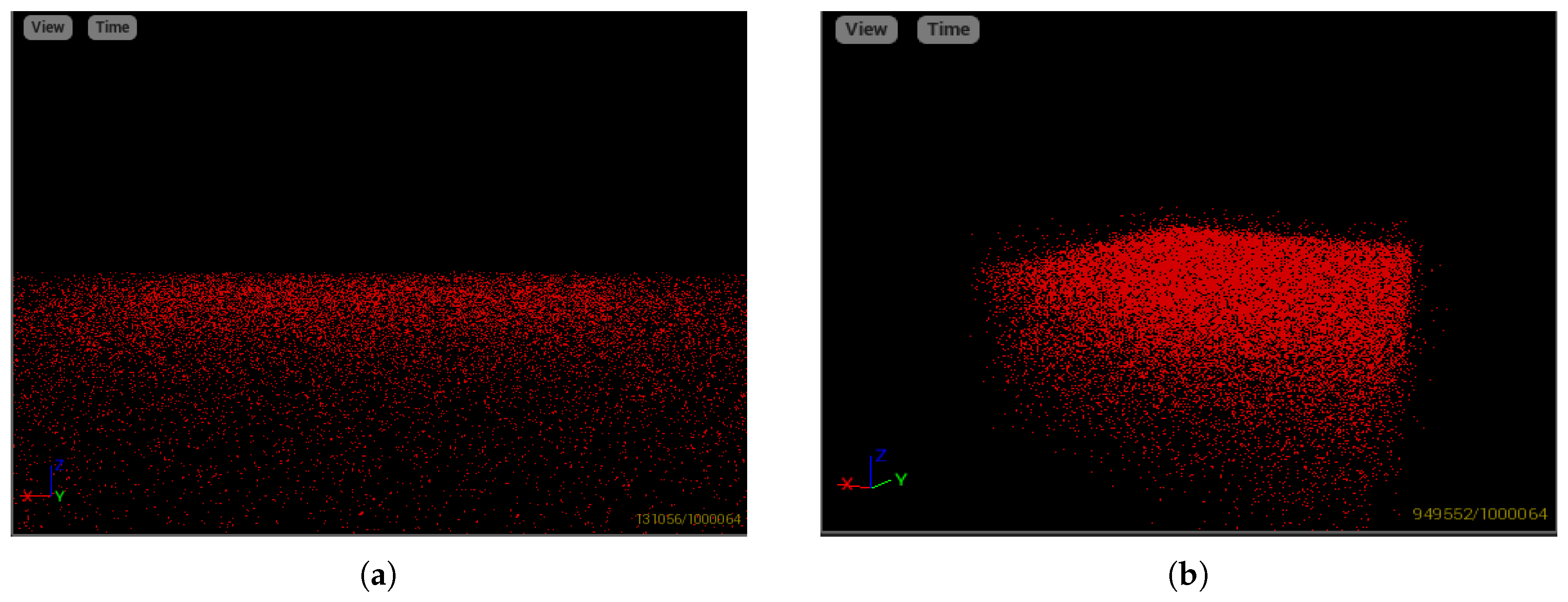
To simulate the plankton’s dynamic behaviour, we chose a flat box shape emitter which will be located close to the surface of the water. The emitter dimension was chosen to be 100 × 100 × 1 m. The XY dimension represents our region of interest due to obvious reasons it cannot be set to infinity. The Z dimension represents the depth and the extent where there is enough sunlight to enable photosynthesis. The initial velocity is chosen to be uniformly distributed where V x U ( 1 , 1 ) , V y U ( 1 , 1 ) , V z U ( 1 , 10 ) . Under these conditions, the plankton will move randomly around the surface of the water with some preference to move to deeper layers. In that case, if the camera is not pointed directly to the emitter, the particles will slowly move in to the field of view of the camera. We assume that there are only small microcurrents that affect the movement of the plankton. This is obviously not always the case but we can later add more emitters that can simulate different underwater currents. The distribution of the particles can be seen in the 2D projection and in the 3D projection given in Figure 20. In those images, we can see that the initial velocity setup gives smooth transition in terms of particle density as we go deeper. This behaviour imitates the natural preference of plankton to the light coming from the surface.
In order to control the number of particles, we choose a uniformly distributed lifetime between 80 to 500 s. The trade-off, in this case, is that since the particles are constantly emitted, we need to control the number of live particles and this is done by the LifeTime parameter. This is obviously different behaviour than a real plankton particle which usually lives much longer than 80 s. However, due to dynamically changing lighting coming from the refraction on the surface of the water, we do occasionally see some sparkling effect which can be simulated with the addition and removal of particles as described above. In terms of visibility, plankton particles constantly move, but in a dynamic scene where the camera is also moving that should not be too significant. In contrast, although having shorter lifetime values will let the particle system stabilize faster it will come with the cost of increasing sparkling effect due to shorter lifetime of the particles and will require more particles to be emitted to preserve the same amount of living particles as with a longer lifetime value.
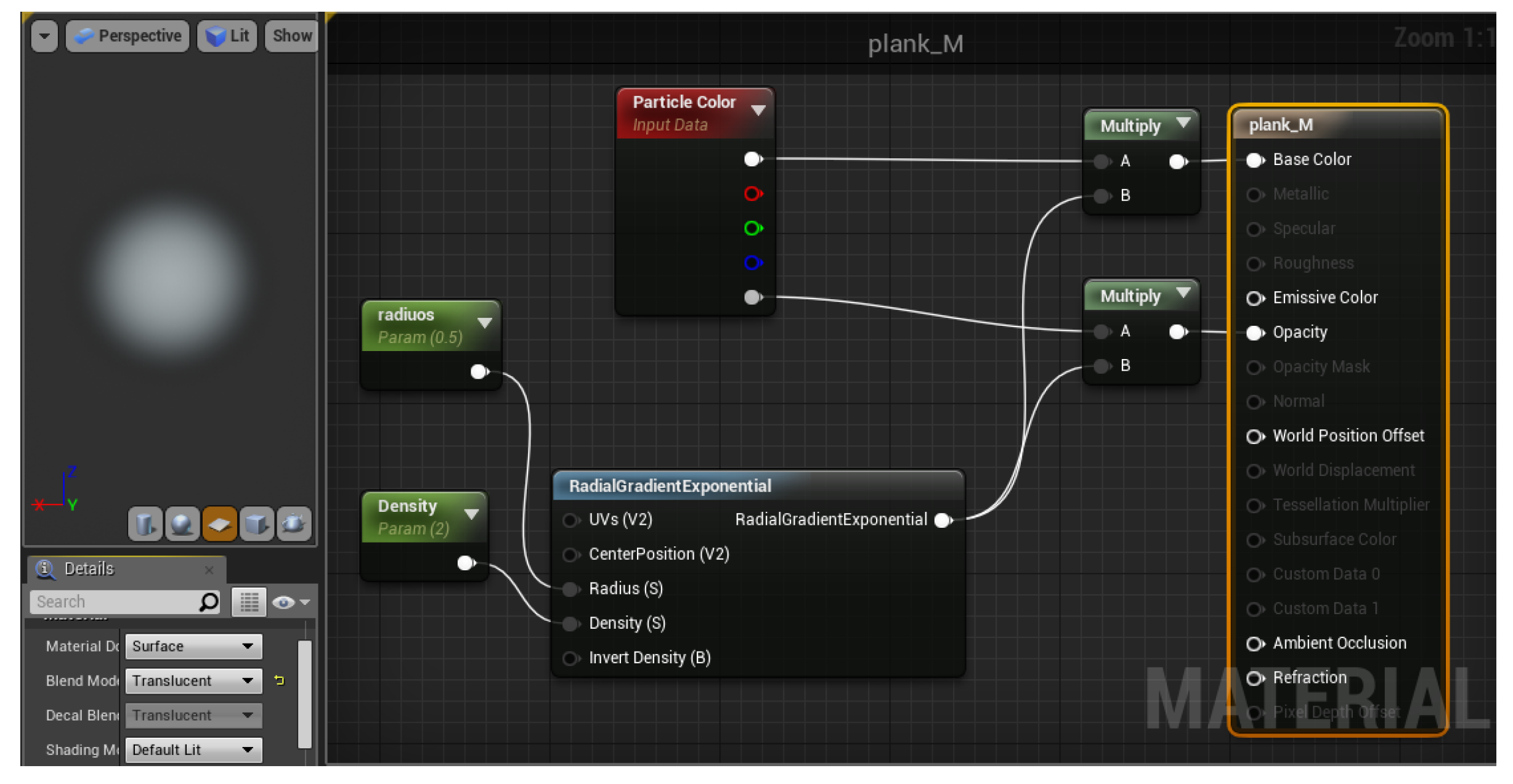
The shape and the texture of the plankton can be complex depending on the type of the organism but since they are still relatively small we use an ellipsoid approximation of the shape. The ellipsoid shape gives us some asymmetry around the middle axes aligned to the world frame which will create an asymmetric backscatter effect. To generate the ellipsoid shape we generated a new material (Figure 21) based on a “RadialGriadientExponential” component which basically means that it exponentially reduces the intensity based on the distance from the centre. The result is then multiplied by the particular colour and fed as a base colour and opacity. The partial opacity makes rendering of the particle to be even more realistic by simulating the transparency of the plankton. In the particle engine, we choose to generate the particles with different random scaling around the X axis. The random scaling together with random initial orientation will create randomly oriented floating ellipsoids. Figure 22 shows the final zooplankton simulation result.
Finally, to simulate motion blur in computer graphics, usually, multiple images or pixels (or subframes) are taken and averaged [44]. The blurring can affect the whole image in case of camera movement or just moving objects inside the field of view if the camera is stable. In the unreal engine, we can control the intensity of the blurring by adjusting the motion blur amount parameter. In Figure 23, we can see a real image that we took underwater as an example of motion blur of plankton and a simulated image done by rotating the simulated camera around the Z axis.

5.4. Test Case Results

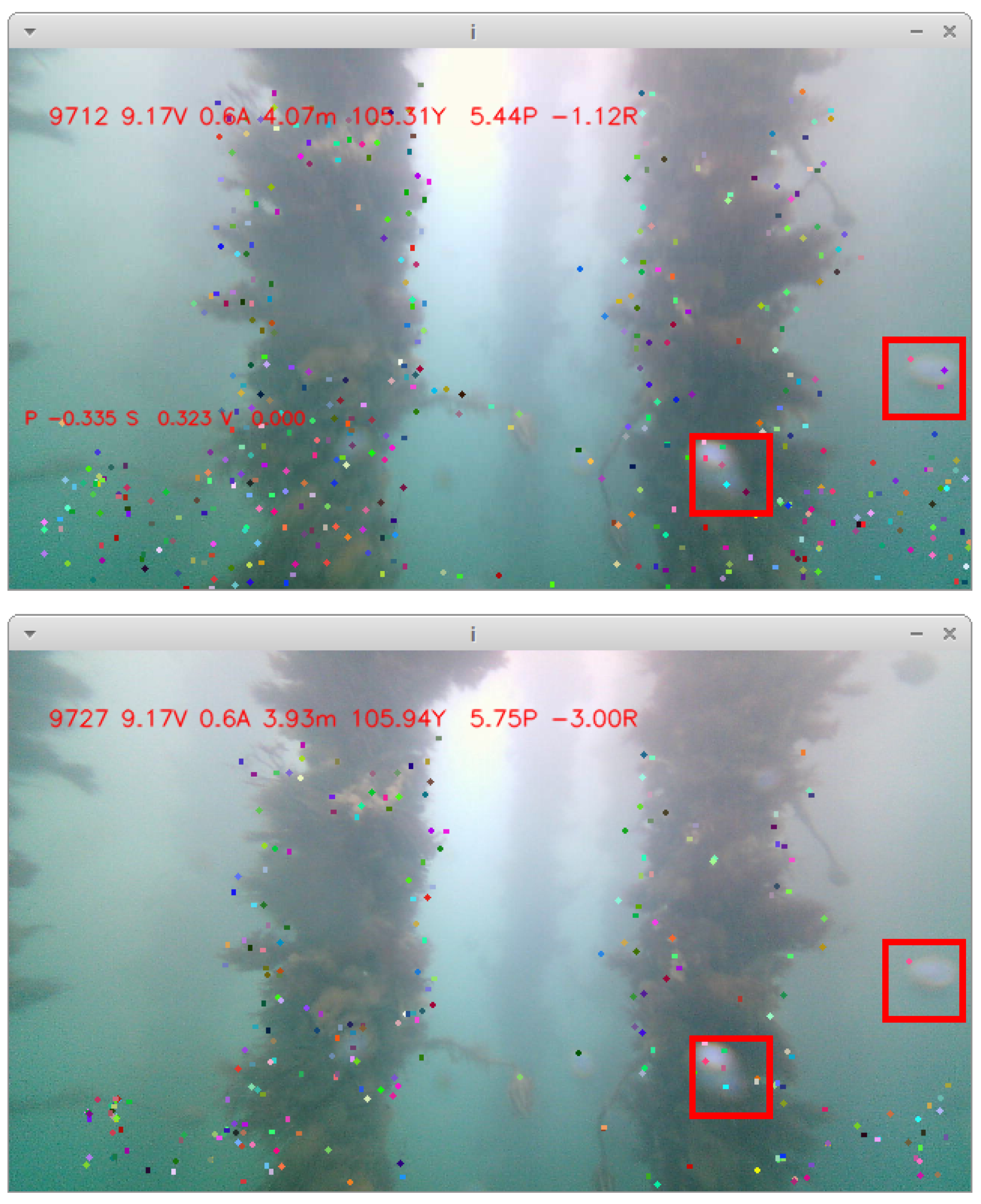
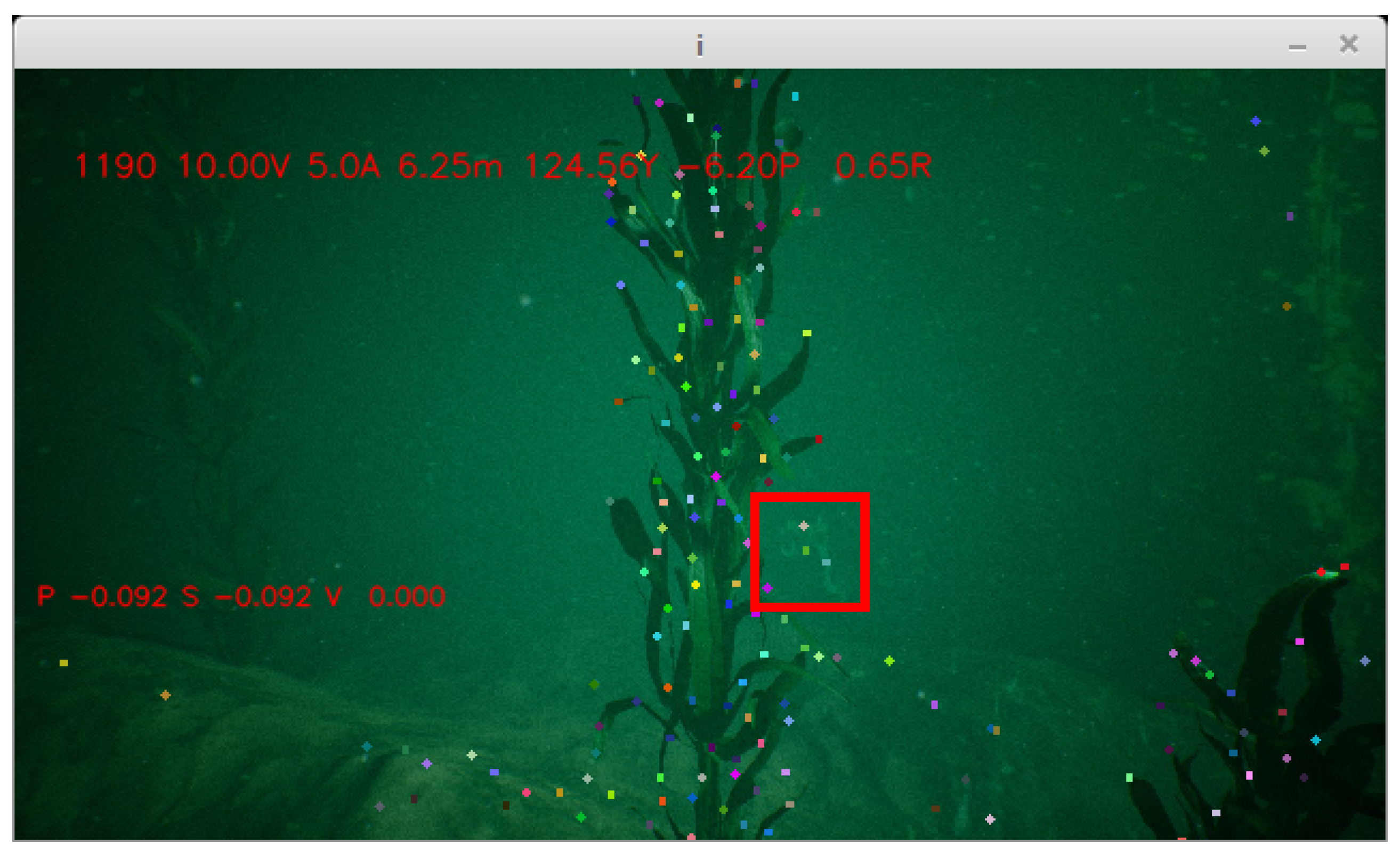
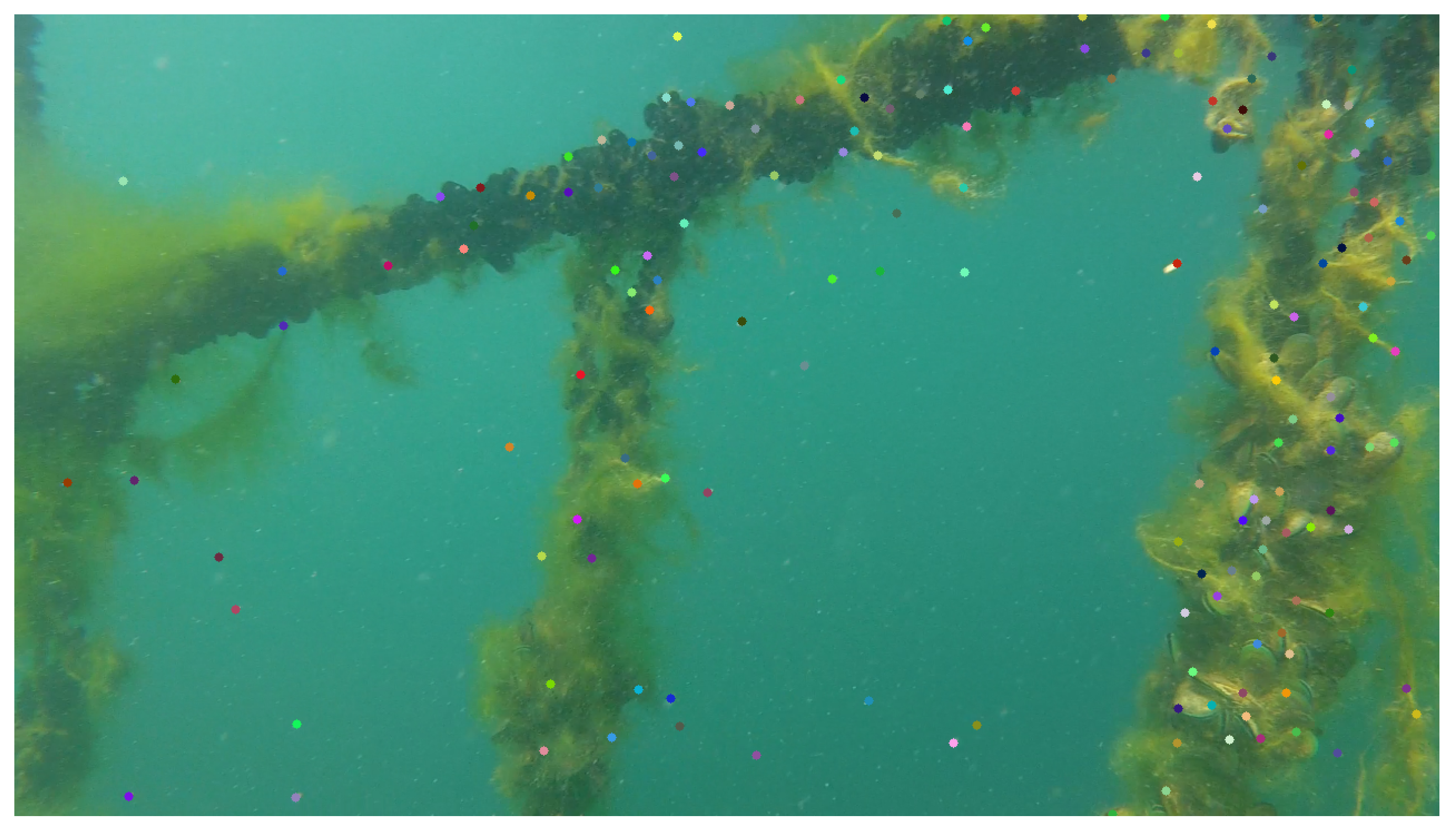
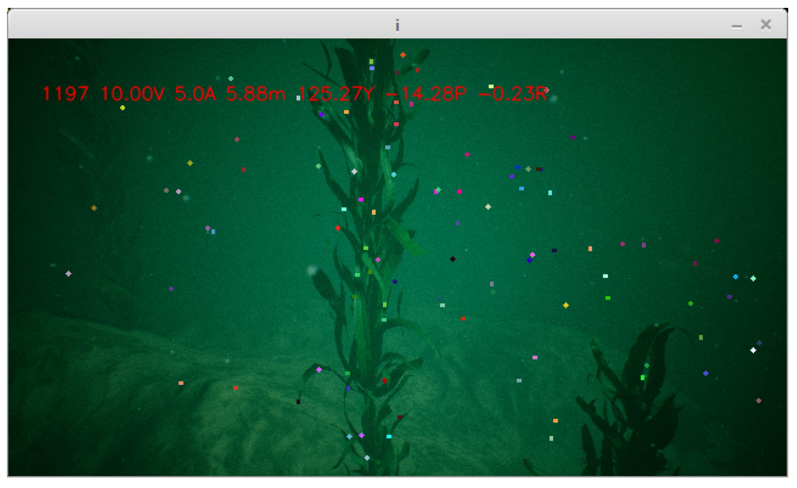
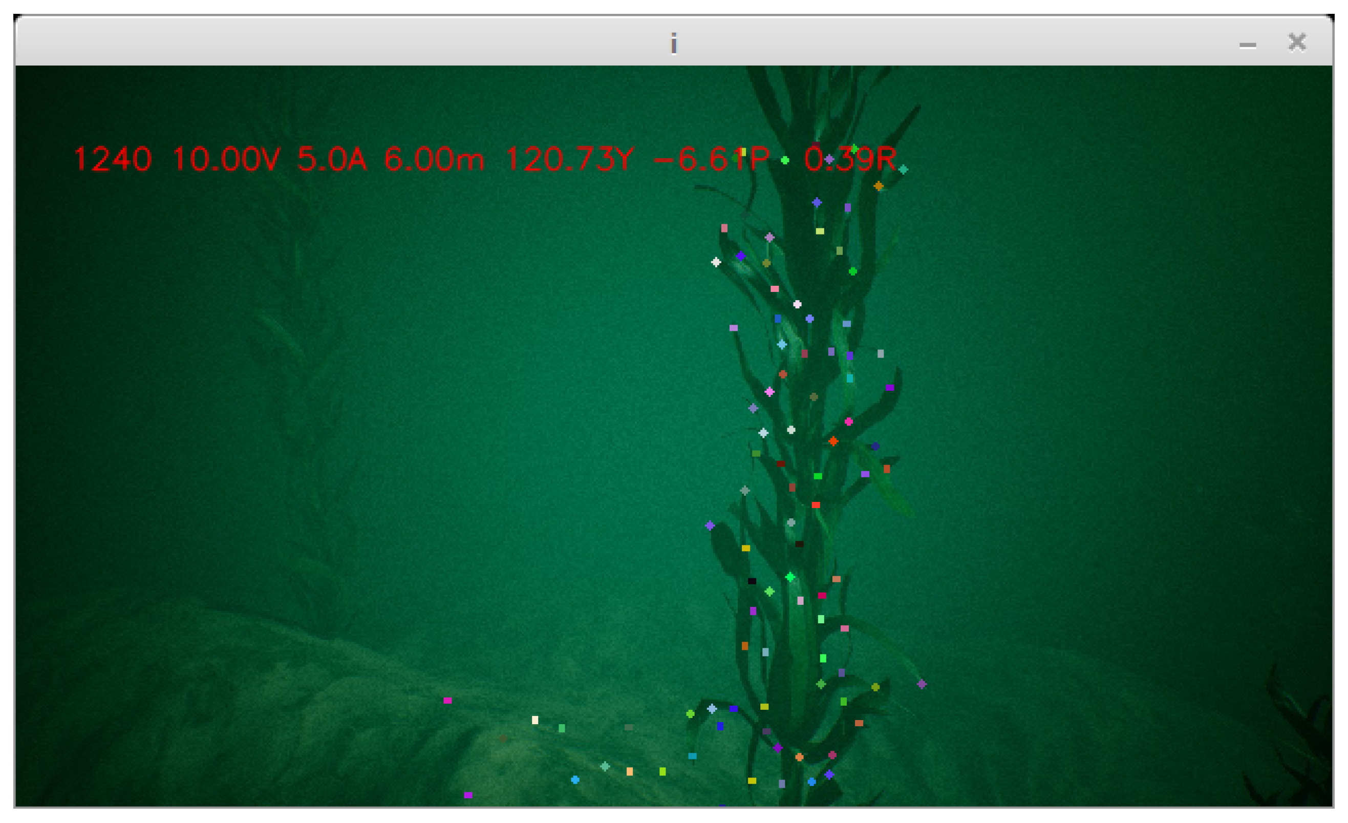
For the purpose of analysing the contribution of the simulated environment, we created a test case algorithm based on the ORB future detection algorithm [45] and optical flow tracking based on [46] implemented in OpenCV. In this experiment, we show that the futures extracted from the scene are not the usually intended futures we would expect and would have an adverse impact on algorithms such as SLAM and obstacle detection which are based on tracking features. In Figure 24, we can see that tracking algorithm treats the dirt bubble as legitimate objects in the scene based on those features there is no camera movement between the frames where in fact we can see (from other features and the objects) that the view is moving upwards. In Figure 25 we can see the same effect repeating in the simulation as we intended. In the real image Figure 26 which we took underwater, we can see features detected in the view not only on the clear visible objects like the ropes but also on the zooplankton and organic material surrounding those ropes. Similarly in the simulated image in Figure 27 we can see features detected on our simulated zooplankton. Since this is a simulated scene we can turn on and off the zooplankton and run the feature detector as presented in Figure 28. In This Figure, we can see that features were detected only on the visible object. We can also see that futures were not detected on the distant objects due to simulated fog which reduces the visible gradients.
In conclusion, this test case experiment sums up the essential concepts and implementation aspects related to the generation of a visually convincing underwater environment simulation. There are many more graphical effects which could not be covered by the scope of the paper and in our simulation but based on our real underwater experience we tried to cover the main effects influencing our underwater scene. The realism of the images was demonstrated by a visual comparison of the simulated images generated using Unreal Engine with real images. Most of the modelling and design aspects used in our work were based on information gathered by watching and experimenting with real underwater systems. We created a computer vision test case algorithm and compared side by side the performance of the algorithm on real images and videos taken during our real test dives with simulated experiments. The outcome showed a convincing similarity between the simulation and the real environment for feature extraction and tracking experiments.

6. Conclusions and Future Research

Although the environment and the visual effects of a state of the art game engine are highly convincing, some complex and important effects were neglected for the sake of simplicity. Similar to ground effects experienced by aeroplanes, we have ground underwater effects both in terms of hydrodynamics when getting close to the constraining floor and also the visual effects like small sand particles moving due to the flow created by the ROV. We hope that by showing the usefulness of this work we will encourage improvements and generation of environments not only for the purpose of gaming but for computer vision research in general, and underwater simulation in particular.
The motivation behind our simulation was effectively demonstrated using a popular underwater ROV which we tested in the real-world and used as a reference to our simulation. We applied computer vision algorithms to test the hypothesis that the created simulated environment and the real environment are compatible to some extent. The computer vision algorithms we test were just a sample and will be interesting to see more algorithms tested under this environment. Due to the high fidelity nature of the simulation, the simulation can serve as a good baseline for comparison between techniques and approaches in computer vision, control algorithms and the combination of both.
Developing an underwater simulation is a multidisciplinary task involving different expertise from the different domains. The existing tools today from the different domains can provide the necessary components. In this paper we covered all the parts which comprise a full-scale simulation. Each part was accompanied by a relevant sub simulation for additional per case tuning. A code reference was provided for reproducibility of the paper results. Video [47] and Figure 29 shows the final result of the simulation which includes the ROV dynamics, the tether simulation and the surrounding underwater environment.
Our future research will focus on building and comparing more complex underwater ROVs with multiple cameras and ROVs with better manoeuvrability compared to the OpenROV. We are also aiming for the comparison of a high level of algorithms which incorporates computer vision together with control algorithms in both simulated and real environments. For example, in our simulation, an autonomous mission can be tested and analysed end to end before applying or even building an ROV. We can use the dynamic section presented in this paper to guide us in designing the ROV and also manipulating the underwater environment we presented for the purpose of that mission. A fully autonomous control algorithm like a seabed scan can be designed and tested under the presented framework.

Author Contributions

O.G., Main author, responsible for the conceptualization, methodology, writing and the software; R.M., provided general guidance, validation of methodologies, editing and writing; R.G., reviewing, editing, general guidance and supervision.

Funding

This research was funded by Callaghan Innovation (a Crown entity of NZ) for the grant, CRS-S7-2017 Precision Farming Technology for Aquaculture.

Conflicts of Interest

The authors declare no conflict of interest.

Appendix A. ROV Dynamics Implementation

In this Appendix we will present a step by step detailed explanation for the simulation of the ROV dynamics. The framework we used for developing the simulation was the Jupyter notebook, an interactive data science and scientific computing platform [29] mainly for the python language. The core tool for this rigid body dynamic simulation is the SymPy Mechanics, a mechanics python package which generates the necessary symbolic equations of motions for our rigid body system [17]. Some additional supporting packages where also used mainly for plotting and for function generation. The full notebook can be accessed and downloaded for further referencing [48].
The following setup shows the necessary software package tools used in this simulation. The abbreviation “me” is used as a synonym for the SymPy mechanics package for compactness.
Listing A1. Setup.
Listing A1. Setup.
import matplotlib.pyplot as plt
from sympy import ∗
import sympy.physics.mechanics as me
from sympy import sin, cos, symbols, solve
from pydy.codegen.ode_function_generators import generate_ode_function
from scipy.integrate import odeint
from IPython.display import SVG
me.init_vprinting(use_latex=’mathjax’)
Next we define the inertial reference frame, the generalized coordinates which are the ROV position and orientation and the subsequent generalized speeds which are the angular and linear velocities.
Listing A2. Symbols definitions.
N = me.ReferenceFrame(’N’) # Inertial Reference Frame
O = me.Point(’O’) # Define a world coordisympynate origin
O.set_vel(N, 0) # Setting world velocity to 0
 
#generelized coordinates
#q0..3 = xyz positions  q4..6 = yaw,pitch,roll rotations
q = list(me.dynamicsymbols(’q0:6’))
 
#generlized speeds
u = list(me.dynamicsymbols(’u0:6’))
 
kin_diff=Matrix(q).diff()-Matrix(u)
In addition we need to define the constants symbols used in our simulation where the geometric aspect of the symbols can be seen in Figure 2:
Listing A3. Constant Symbols Definition.
Wx = symbols(’W_x’)
Wh = symbols(’W_h’)
T1 = symbols(’T_1’)
T2 = symbols(’T_2’)
Bh = symbols(’B_h’)
Bw = symbols(’B_w’)
m_b = symbols(’m_b’) # Mass of the body
v_b = symbols(’v_b’) # Volume of the body
mu = symbols(’\mu’) #drag
mu_r = symbols(’\mu_r’) #rotational drag
g = symbols(’g’)
I = list(symbols(’Ixx, Iyy, Izz’)) #Moments of inertia of body
The ROV reference frame is defined by subsequent Euler angles rotations with respect to the inertial frame:
Listing A4. ROV reference frame.
Rz=N.orientnew(’R_z’, ’Axis’, (q[3+2], N.z))
Rz.set_ang_vel(N,u[3+2]∗N.z)
 
Ry=Rz.orientnew(’R_y’, ’Axis’, (q[3+1], Rz.y))
Ry.set_ang_vel(Rz,u[3+1]∗Rz.y)
 
R=Ry.orientnew(’R’, ’Axis’, (q[3+0], Ry.x))
R.set_ang_vel(Ry,u[3+0]∗Ry.x)
In order to apply gravity and buoyancy forces we need to define the COM (Center Of Mass) and COB (Center Of Buoyancy) in the reference frame.
Listing A5. COM and COB in the reference frame R.
# Center of mass of body
COM = O.locatenew(’COM’, q[0]∗N.x + q[1]∗N.y + q[2]∗N.z)
 
# Set the velocity of COM
COM.set_vel(N, u[0]∗N.x + u[1]∗N.y + u[2]∗N.z)
 
# center of bouyency
COB = COM.locatenew(’COB’, R.x∗Bw+R.z∗Bh)
COB.v2pt_theory(COM, N, R);
As an input to the Kane method [11] we need to calculate the inertia dyadic or matrix. The next listing defines the rigid body for the Kane equations with the relevant inertia symbols:
Listing A6. Rigid Body defenitions.
Ib = me.inertia(R, ∗I , ixy=0, iyz=0, izx=0)
Body = me.RigidBody(’Body’, COM, R, m_b, (Ib, COM))
Next we define the drag forces that influencing the underwater ROV.
Listing A7. Rigid Body Drag.
v=N.x∗u[0]+N.y∗u[1]+N.z∗u[2]
Fd=-v∗mu
T_z=(R,-u[3+2]∗N.z∗mu_r)
T_x=(R,-u[3+0]∗Rz.x∗mu_r)
T_y=(R,-u[3+1]∗Rx.y∗mu_r) #rotaional dumping Torqe
The following are the buoyancy and gravity constant forces and the thrusters forces. The definition of theses forces is straightforward as can be seen in the following listing:
Listing A8. External Forces.
Fg = -N.z ∗ m_b ∗ g # gravity
Fb = N.z ∗ v_b ∗ 1e3 ∗g # buoyancy
F1, F2, F3 = symbols(’f_1, f_2, f_3’) # thrusters
The next listing shows the final kane’s step implemented in the simulation including the integration step:
Listing A9. Kanes Final Step.
 
#multiplying by inverse mass matrix:
u_dot=kane.mass_matrix.inv()∗kane.forcing
 
#replacing the constants with actual numerical values:
subs=[(Wx,0.1), (Wh,0.15), (T1,0.1), (T2,0.05),
  (Bh,0.08), (Bw,0.01), (m_b,1.0), (v_b,0.001),
  (mu,0.3), (mu_r,0.2), (g,9.8), (I[0],0.5),
  (I[1],0.5), (I[2],0.5) ]
u_dot_simp=u_dot.subs(subs)
u_dot_simp=trigsimp(u_dot_simp)
 
#generating a lambda function to compute the values of the u_dot vector
from sympy import lambdify
def get_next_state_lambda(subs):
  u_dot_simp_q_u_f=u_dot_simp.subs(subs)
  return lambdify((q,u,F1,F2,F3),u_dot_simp_q_u_f)
 
#integrating function which takes the current state and returns the next state
def get_next_state(curr_q,curr_u,control,curr_t,dt,lamb):
  forces=control(curr_t)
  u_dot_f=lamb(curr_q,curr_u,∗forces).flatten()
  next_q=curr_q+curr_u∗dt
  next_u=curr_u+u_dot_f∗dt
  return next_q,next_u
We can see the the kane’s methods provides us with the final u ˙ term which we can be use as seen by the previous listing. The next equations summarize the final result of our dynamic simulation. This equation obtained automatically from the SymPy framework after replacing the constant symbols with the matching numerical values:
u ˙ ( u , q , f ) = 1.0 f 1 cos q 4 cos q 5 + 1.0 f 2 cos q 4 cos q 5 + 1.0 f 3 sin q 3 sin q 5 + sin q 4 cos q 3 cos q 5 0.3 u 0 1.0 f 1 sin q 5 cos q 4 + 1.0 f 2 sin q 5 cos q 4 + 1.0 f 3 sin q 3 cos q 5 + sin q 4 sin q 5 cos q 3 0.3 u 1 1.0 f 1 sin q 4 1.0 f 2 sin q 4 + 1.0 f 3 cos q 3 cos q 4 0.3 u 2 2.0 0.2 u 3 cos q 4 + 0.5 u 4 u 5 0.784 sin q 3 cos q 4 + 2.0 0.1 f 1 cos q 3 cos q 4 + 0.1 f 2 cos q 3 cos q 4 + 0.05 f 3 sin q 3 cos q 4 + 0.5 u 3 u 4 cos q 4 + 0.2 u 3 sin q 4 0.2 u 5 sin q 4 cos 2 q 4 0.2 f 1 sin q 3 0.2 f 2 sin q 3 + 0.1 f 3 cos q 3 1.0 u 3 u 5 cos q 4 0.4 u 4 1.568 sin q 4 cos q 3 0.196 cos q 4 0.2 f 1 cos q 3 cos q 4 + 0.2 f 2 cos q 3 cos q 4 + 0.1 f 3 sin q 3 cos q 4 + 1.0 u 3 u 4 cos q 4 + 1.0 u 4 u 5 tan q 4 0.4 u 5 cos 2 q 4 1.568 sin q 3 tan q 4
We can see from this equation that u ˙ is a function of u, q and f and can be used iteratively as the integration step. Finally, in order to use the dynamic simulation inside a full scale 3d simulation we only need to save the mid products of the simulation to a packed file. In the python programming language this can be done using the pickle library. The file can be later uploaded to memory and we can regenerate the lambda function for getting the u ˙ vector for the iterative integration.

References

  1. Fahlstrom, P.; Gleason, T. Introduction to UAV Systems; John Wiley & Sons: Hoboken, NJ, USA, 2012. [Google Scholar]
  2. AirSim, Simulator for Drones. 2016. Available online: https://github.com/microsoft/airsim/ (accessed on 21 December 2018).
  3. NVIDIA DRIVE CONSTELLATION. 2018. Available online: https://www.nvidia.com/en-us/self-driving-cars/drive-constellation/ (accessed on 21 December 2018).
  4. Underwater Simulation. Available online: https://github.com/uji-ros-pkg/underwater_simulation (accessed on 21 December 2018).
  5. Kermorgant, O. A dynamic simulator for underwater vehicle-manipulators. In Proceedings of the International Conference on Simulation, Modeling, and Programming for Autonomous Robots, Bergamo, Italy, 20–23 October 2014; pp. 25–36. [Google Scholar]
  6. Multi-ROV Training Simulator. Available online: http://marinesimulation.com/rovsim-gen3/ (accessed on 21 December 2018).
  7. Myint, M.; Yonemori, K.; Lwin, K.N.; Yanou, A.; Minami, M. Dual-eyes vision-based docking system for autonomous underwater vehicle: An approach and experiments. J. Intell. Robot. Syst. 2018, 92, 159–186. [Google Scholar] [CrossRef]
  8. Myint, M.; Yonemori, K.; Yanou, A.; Ishiyama, S.; Minami, M. Robustness of visual-servo against air bubble disturbance of underwater vehicle system using three-dimensional marker and dual-eye cameras. In Proceedings of the IEEE OCEANS’15 MTS/IEEE, Washington, DC, USA, 19–22 October 2015; pp. 1–8. [Google Scholar]
  9. Ganoni, O.; Mukundan, R.; Green, R. Visually Realistic Graphical Simulation of Underwater Cable. In Proceedings of the 26th International Conference in Central Europe on Computer Graphics, Visualization and Computer Vision, Plzen, Czech, 28 May–1 June 2018. [Google Scholar]
  10. Ganoni, O.; Mukundan, R. A Framework for Visually Realistic Multi-robot Simulation in Natural Environment. arXiv, 2017; arXiv:1708.01938. [Google Scholar]
  11. Mechanics, S.C. Kane Method Implementation. Available online: http://docs.sympy.org/latest/modules/physics/mechanics/kane.html (accessed on 21 December 2018).
  12. SymPy. Available online: http://docs.sympy.org (accessed on 21 December 2018).
  13. Kane, T.R.; Levinson, D.A. Dynamics, Theory and Applications; McGraw Hill: New York, NY, USA, 1985; Chapter 7; pp. 30–31. [Google Scholar]
  14. Kane, T.R.; Levinson, D.A. Dynamics, Theory and Applications; McGraw Hill: New York, NY, USA, 1985. [Google Scholar]
  15. Batchelor, G.K. An Introduction to Fluid Dynamics; Cambridge University Press: Cambridge, UK, 2000; pp. 233–245. [Google Scholar]
  16. Kane, T.R.; Levinson, D.A. Dynamics, Theory and Applications; McGraw Hill: New York, NY, USA, 1985; Chapter 6; pp. 158–159. [Google Scholar]
  17. SymPy Mechanics. Available online: http://docs.sympy.org/latest/modules/physics/mechanics/index.html (accessed on 21 December 2018).
  18. Kane, T.R.; Levinson, D.A. Dynamics, Theory and Applications; McGraw Hill: New York, NY, USA, 1985; Chapter 7; pp. 204–205. [Google Scholar]
  19. Bender, J.; Müller, M.; Otaduy, M.A.; Teschner, M.; Macklin, M. A survey on position-based simulation methods in computer graphics. Comput. Graph. Forum 2014, 33, 228–251. [Google Scholar] [CrossRef]
  20. Macklin, M.; Müller, M. Position based fluids. ACM Trans. Graph. (TOG) 2013, 32, 104. [Google Scholar] [CrossRef]
  21. Jakobsen, T. Advanced character physics. In Proceedings of the Game Developers Conference, San Jose, CA, USA, 22 March 2001; Volume 3. [Google Scholar]
  22. Marshall, R.; Jensen, R.; Wood, G. A general Newtonian simulation of an n-segment open chain model. J. Biomech. 1985, 18, 359–367. [Google Scholar] [CrossRef]
  23. Cable Component in Unreal Engine 4. Available online: https://docs.unrealengine.com/latest/INT/Engine/Components/Rendering/CableComponent/ (accessed on 21 December 2018).
  24. Verlet, L. Computer “experiments” on classical fluids. I. Thermodynamical properties of Lennard-Jones molecules. Phys. Rev. 1967, 159, 98. [Google Scholar] [CrossRef]
  25. OpenRov. Available online: https://www.openrov.com/ (accessed on 21 December 2018).
  26. Cable Simulation Video. 2018. Available online: https://youtu.be/_QoMUSlQCsg (accessed on 21 December 2018).
  27. Underwater Cable Reel Simulation Video. 2018. Available online: https://youtu.be/DO-x2RaZHso (accessed on 21 December 2018).
  28. Cable Sim Project. 2018. Available online: https://github.com/UnderwaterROV/UWCableComponent (accessed on 21 December 2018).
  29. Jupyter. Available online: http://jupyter.org/ (accessed on 21 December 2018).
  30. Cable Sim Notebook. 2018. Available online: https://github.com/UnderwaterROV/underwaterrov/blob/master/notebooks/rope.ipynb (accessed on 21 December 2018).
  31. Lalli, C.; Parsons, T.R. Biological Oceanography: An Introduction; Butterworth-Heinemann: Oxford, UK, 1997. [Google Scholar]
  32. Capuzzo, E.; Stephens, D.; Silva, T.; Barry, J.; Forster, R.M. Decrease in water clarity of the southern and central North Sea during the 20th century. Glob. Chang. Biol. 2015, 21, 2206–2214. [Google Scholar] [CrossRef] [PubMed] [Green Version]
  33. Haltrin, V.I. Chlorophyll-based model of seawater optical properties. Appl. Opt. 1999, 38, 6826–6832. [Google Scholar] [CrossRef] [PubMed]
  34. Jaffe, J.S.; Moore, K.D.; McLean, J.; Strand, M.P. Underwater optical imaging: Status and prospects. Oceanography 2001, 14, 66–76. [Google Scholar] [CrossRef]
  35. Pope, R.M.; Fry, E.S. Absorption spectrum (380–700 nm) of pure water. II. Integrating cavity measurements. Appl. Opt. 1997, 36, 8710–8723. [Google Scholar] [CrossRef] [PubMed]
  36. Buiteveld, H.; Hakvoort, J.; Donze, M. Optical properties of pure water. In Proceedings of the Ocean Optics XII, Bergen, Norway, 13–15 June 1994; Volume 2258, pp. 174–184. [Google Scholar]
  37. Thibos, L.; Bradley, A.; Still, D.; Zhang, X.; Howarth, P. Theory and measurement of ocular chromatic aberration. Vis. Res. 1990, 30, 33–49. [Google Scholar] [CrossRef]
  38. Unreal Engine 4 Chromatic Aberration. Available online: https://docs.unrealengine.com/latest/INT/Engine/Rendering/PostProcessEffects/SceneFringe/ (accessed on 21 December 2018).
  39. Ocean Floor Environment. Available online: https://www.unrealengine.com/marketplace/ocean-floor-environment (accessed on 21 December 2018).
  40. Unreal Engine 4 SimpleGrassWind. Available online: https://docs.unrealengine.com/en-us/Engine/Rendering/Materials/Functions/Reference/WorldPositionOffset (accessed on 21 December 2018).
  41. Exponential Height Fog User Guide. Available online: https://docs.unrealengine.com/latest/INT/Engine/Actors/FogEffects/HeightFog/index.html (accessed on 21 December 2018).
  42. NatGeoPauly-Freshwater Fish Feeding on Plankton “Peacock Bass”. 2014. Available online: https://www.youtube.com/watch?v=JAd2jZuNkd8 (accessed on 21 December 2018).
  43. Unreal Engine 4 Particle Systems. Available online: https://docs.unrealengine.com/latest/INT/Engine/Rendering/ParticleSystems/ (accessed on 21 December 2018).
  44. Schroeder, W.J.; Lorensen, B.; Martin, K. The Visualization Toolkit: An Object-Oriented Approach to 3D Graphics; Kitware: Clifton Park, NY, USA, 2004. [Google Scholar]
  45. Rublee, E.; Rabaud, V.; Konolige, K.; Bradski, G. ORB: An efficient alternative to SIFT or SURF. In Proceedings of the 2011 IEEE International Conference on Computer Vision (ICCV), Barcelona, Spain, 6–13 November 2011; pp. 2564–2571. [Google Scholar]
  46. Bouguet, J.Y. Pyramidal implementation of the affine lucas kanade feature tracker description of the algorithm. Intel Corp. 2001, 5, 4. [Google Scholar]
  47. Underwater Simulation. 2018. Available online: https://youtu.be/MP2xG_Tms3E (accessed on 21 December 2018).
  48. ROV Dynamics Notebook. 2018. Available online: https://github.com/UnderwaterROV/underwaterrov/blob/master/notebooks/openrov_sim.ipynb (accessed on 21 December 2018).
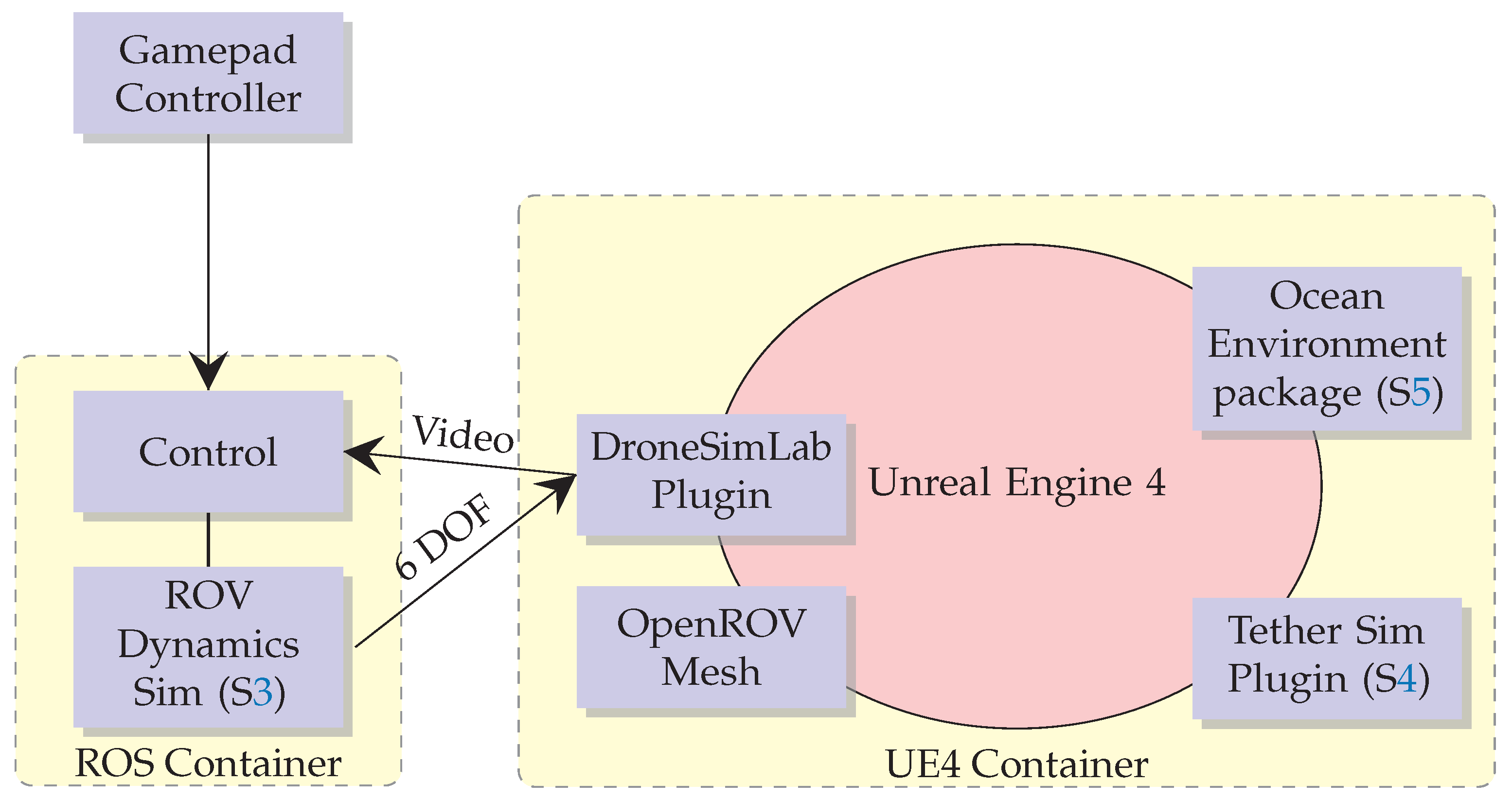
Figure 1. Simulation Diagram. This diagrams shows the components of the simulation and the main communication channels. S4, S5 and S3 refers to the relevant sections in this paper.
Drones 03 00001 g001
Figure 2. Schematic drawing of the OpenROV where: m A : Mass of the ROV. T 1 : Distance from center of mass (COM) to back thruster axis. T 2 : Distance from COM to upper thruster axis. W x : distance from center axis to back thruster axis. W h : distance from center axis to upper thruster. B h : the z measure of center of buoyancy (COB) distance from COM. B x : the x measure of COB distance from COM. L 1 . . 3 : Position points of the thrusters.
Drones 03 00001 g002
Figure 3. Simulation result summery. (a) shows position over time; (b) shows rotations over time Euler angels Yaw, Pitch and Roll; (c) a projected course of the ROV in the X-Y plane; (d) shows the angular velocities around the X, Y and Z axis.
Drones 03 00001 g003
Figure 4. The underwater ROV sees its own tether in the camera view. On the left is an image taken from our simulation and on the right an image taken from one of our dives with the OpenROV in Port Levy, New Zealand.
Drones 03 00001 g004
Figure 5. This figure shows the variation of the total cable length in meters with respect to the frame number. We can see that when using 10 solver constrain iterations (per frame) to enforce the distance constraint of each cable segment the cable maintains its overall length more and represents a less stretchable cable.
Drones 03 00001 g005
Figure 6. Length constraints and bending constraints. We can see at this diagram an example to the constraints apply on the cable segments. For example between adjacent points like E and F we require L distance which will create resistance to stretch and between points with one vertex between them like A and C we require 2 L distance which will cause resistance to stretching with additional resistance to bending.
Drones 03 00001 g006
Figure 7. A small underwater OpenROV robot connected through a thin cable for video and control transmissions [25].
Drones 03 00001 g007
Figure 8. Unreal Engine 4 editor environment.
Drones 03 00001 g008
Figure 9. Experimental verification of motion of an extensible cable. We colored the cable in a checkers like pattern to enable the extension of the cable to be observable.
Drones 03 00001 g009
Figure 10. A 2D model of a flexible cable where one of the end points A is moved with a constant velocity v towards a target S.
Drones 03 00001 g010
Figure 11. The damping effect. This figure shows the cable in different times. In t = 0 we start to move the edge of the cable in the direction up and right along the “xy” plane. The first figure shows the results without damping and the second shows the behaviour of that cable with damping coefficient of 0.98. We can clearly see that the damping is absorbing the wave energy as we would expect in aquatic systems.
Drones 03 00001 g011
Figure 12. Damping with 0.9 coefficient. Tuning the coefficient to 0.9 causes the desired effect for underwater simulation in the case of a low tension cable in an underwater environment. Disturbance on one side remains local.
Drones 03 00001 g012
Figure 13. Introducing random forces to the system. Both images show the cable state after the system is stabilized ( t > > 0 ). The first and the second images show the cable state with and without random forces respectively. We can see the “Memory Loss” that we would expect to see in a marine-like environment with underwater currents.
Drones 03 00001 g013
Figure 14. We took this underwater image during daylight in Pelorus Sound New Zealand to demonstrate the challenges of modelling realistic underwater imagery. The image shows significant amount of organic material and reflections from the plankton. We can also observe the mist effect created by the phytoplankton.
Drones 03 00001 g014
Figure 15. Absorption coefficient versus Wavelength. Logarithmic plot showing the absorption coefficient of fresh water [35,36].
Drones 03 00001 g015
Figure 16. A sea weed dynamic simulation based on grass wind.
Drones 03 00001 g016
Figure 17. Effective FOV underwater. A ray is coming from an angle of θ 2 is refracted with an angle θ 1 which moving the Focal point F a i r to the effective F w a t e r .
Drones 03 00001 g017
Figure 18. Dirt mask added to the simulation. This dirt mask was added to simulate dirt accumulated on the camera port.
Drones 03 00001 g018
Figure 19. Simulating phytoplankton mist. The upper image is a real image taken underwater in Florida’s east side [42]. The bottom image was simulated using Unreal Engine’s “Exponential Height Fog” component. In both images, we can see the distance attenuation effect of the fog where distant objects are less visible. Both images used the sunlight as the main source of light.
Drones 03 00001 g019
Figure 20. View of the particle emitter setup as a flat rectangular box with initial velocities pointing to the negative Z axis direction. (a) shows the particles in the X-Y plane. (b) shows a 3D view of the box emitter setup.
Drones 03 00001 g020
Figure 21. A blueprint of the zooplankton material in the Unreal Engine’s material editor. The left pane shows the final result and on the right the generator blueprint of the plankton material. The RadialGradientExponential component is multiplied by the particle colour (input to the blueprint) and fed as a basic colour an opacity.
Drones 03 00001 g021
Figure 22. Simulated Zooplankton of different sizes and shape. The zooplankton have the appearance of snowflakes with some backscatter illumination. The scene uses a strobe light and sunlight.
Drones 03 00001 g022
Figure 23. Motion blur. (a) is a real image (Pelorus Sound New Zealand) taken when we lowered the camera into the water. We can see the short lines blurring patterns of the Zooplankton due to that movement. (b) A simulated image. This image was created by rotating the simulated camera and setting the motion blur effect in the unreal engine.
Drones 03 00001 g023
Figure 24. Tracking Experiment. This experiment was a real experiment done using the OpenROV platform in a mussel farm near Port Levy New Zealand. Two frames from a tracking experiment, the first number in the telemetry line (upper left corner of each frame) is the frame number. The features in the frames are coloured with different colours in order to keep track. Marked in red square are dirt bubbles attached to the camera port.
Drones 03 00001 g024
Figure 25. Tracking dirt mask. Repeating the experiment done in Figure 24 in the simulation. Similar to Figure 24 we can sea that features are detected and tracked on the dirt mask (mark in red square).
Drones 03 00001 g025aDrones 03 00001 g025b
Figure 26. Running feature extraction using ORB detector. This real image we took in a mussel farm in marlborough sounds New Zealand. We can see that the features (marked with different colours) were not necessarily detected on the mussel rope but rather on the surrounding organic material.
Drones 03 00001 g026
Figure 27. Feature extraction in a simulated image with zooplankton but without dirt mask.
Drones 03 00001 g027
Figure 28. Feature extraction in a simulated image without zooplankton and without dirt mask. This image shows that as expected no feature where detected on the surrounding medium but only on the front sea weed.
Drones 03 00001 g028
Figure 29. Final simulation result. Running the simulation opens three windows. The left window is showing an outside view of the simulated ROV including the tether. The images on the right are the images from the simulated camera attached to the ROV (one image is with annotations and the other without). The ROV is controlled using an outside gamepad.
Drones 03 00001 g029