Abstract
Developing methods for autonomous landing of an unmanned aerial vehicle (UAV) on a mobile platform has been an active area of research over the past decade, as it offers an attractive solution for cases where rapid deployment and recovery of a fleet of UAVs, continuous flight tasks, extended operational ranges, and mobile recharging stations are desired. In this work, we present a new autonomous landing method that can be implemented on micro UAVs that require high-bandwidth feedback control loops for safe landing under various uncertainties and wind disturbances. We present our system architecture, including dynamic modeling of the UAV with a gimbaled camera, implementation of a Kalman filter for optimal localization of the mobile platform, and development of model predictive control (MPC), for guidance of UAVs. We demonstrate autonomous landing with an error of less than 37 cm from the center of a mobile platform traveling at a speed of up to 12 m/s under the condition of noisy measurements and wind disturbances.
1. Introduction
Over the last few decades, unmanned aerial vehicles (UAVs) have had significant development in many aspects, including fixed-wing designs, hovering multi-copters, sensor technology, real-time algorithms for stabilization and control, autonomous waypoint navigation. In recent years, Micro-UAVs (weight ≤ 3 kg), also known as Micro Aerial Vehicles (MAVs) have had wide adoption in many applications, including aerial photography, surveillance, reconnaissance, and environmental monitoring, to name a few. Although MAVs are highly effective for such applications, they still face many challenges, such as a short operational range and limited computational power of the onboard processors, mainly due to their battery life and/or limited payload. Most MAVs currently in use usually employ a rechargeable lithium polymer (LiPo) battery that can provide a higher energy density than other battery types, but they still have a very limited flight endurance of about 10–30 min at best.
To overcome these issues, a number of solutions have been proposed, including integration of a tether for power and data transmission [1], autonomous deployment and recovery from a charging station [2], solar-powered photovoltaic (PV) panels [3], and development of batteries with high-power density. The most straightforward approach, without a doubt, would be to increase battery capacity, such as with a lightweight hydrogen fuel cell [4], but such batteries are still expensive and heavy for small-scale UAVs. Alternatively, tethered flights with a power transmission line can support hypothetically large-scale flight endurance; however, the operational range of tethered flight is intrinsically limited to the length of the power line. The solar panel methods are attractive for relatively large fixed-wing UAVs, but they are not quite suitable for most rotary-wing UAVs.
Autonomous takeoff from and landing on a mobile platform with a charging or battery swapping station offers an attractive solution in circumstances where continuous flight tasks with an extended operational range are desired. In these scenarios, the UAV becomes an asset to the ground vehicle, where the UAV can provide aerial services such as mapping for the purposes of path planning. For example, emergency vehicles, delivery trucks, and marine or ground carriers could be used for deploying UAVs between locations of interest and as mobile charging stations [2,5,6,7].
Other examples, especially for large-scale UAVs, include autonomous takeoff and landing on a moving aircraft carrier or a naval ship [8,9,10]. Autonomous takeoff and landing also allow more efficient deployment and recovery for a large fleet of UAVs without human intervention.
In this paper, we present a complete system architecture enabling a commercially available micro-scale quadrotor UAV to land autonomously on a high-speed mobile landing platform under various wind disturbances. To this end, we have developed an efficient control method that can be implemented on an embedded system at low cost, power, and weight. Our approach consists of (i) vision-based target position measurement; combined with (ii) a Kalman filter for optimal target localization; (iii) model predictive control for guidance of the UAV; and (iv) integral control for robustness.
The rest of the paper is organized as follows. In Section 2 we discuss various techniques associated with autonomous UAV landing. In Section 3 we present the overall system architecture. Section 4 presents the dynamic model of the UAV for this study, optimal target localization for the landing platform, and the model predictive control for the UAV. Section 5 presents simulation results to validate our approach, and we conclude in Section 6.
2. Related Work
The major challenges in autonomous landing are (i) accurate measurements (or optimal estimates) of the locations of the landing platform as well as the UAV and (ii) robust trajectory following in the presence of disturbances and uncertainties. To face these challenges, several approaches for autonomous landing of rotary-wing UAVs have been proposed. Erginer and Altug have proposed a PD controller design for attitude control combined with vision-based tracking that enables a quadcopter to land autonomously on a stationary landing pad [11]. Voos and Nourghassemi have presented a control system consisting of an inner loop attitude control using feedback linearization, an outer loop velocity and altitude control using proportional control, and a 2D-tracking controller based on feedback linearization for autonomous landing of a quadrotor UAV on a moving platform [12]. Ahmed and Pota have introduced an extended backstepping nonlinear controller for landing of a rotary wing UAV using a tether [13].
Robust control techniques also have been used for UAV landing to deal with uncertain system parameters and disturbances. Shue and Agarwal have employed a mixed control technique, where the method is used for trajectory optimization and the technique minimizes the effect of the disturbance on the performance output [14]. Wang et al. have also employed a mixed technique to ensure that the UAV tracks the desired landing trajectory under the influence of uncertainties and disturbances [15]. In their approach, the method has been formulated as a linear quadratic Gaussian (LQG) problem for optimal dynamic response and the method has been adopted to minimize the ground effect and atmospheric disturbances.
Computer vision has been used in a crucial role in many autonomous landing techniques. Lee et al. [16] have presented image-based visual servoing (IBVS) to track a landing platform in two-dimensional image space. Serra et al. [17] have also adopted dynamic IBVS along with a translational optimal flow for velocity measurement. Borowczyk et al. [18] have used AprilTags [19], a visual fiducial system, together with an IMU and GPS receiver integrated on a moving target travelling at a speed of up to 50 km/h. Beul et al. [20] have demonstrated autonomous landing on a golf cart running at a speed of ~4.2 m/s using two cameras for high-frequency pattern detection in combination with an adaptive yawing strategy.
Learning-based control methods for autonomous landing have also been studied to achieve the optimal control policy under uncertainties. Polvara et al. [21] have proposed an approach based on a hierarchy of deep Q-networks (DQNs) that can be used as a high-end control policy for the navigation in different phases. With an optimal policy, they have demonstrated a quadcopter autonomously landing in a large variety of simulated environments. A number of approaches based on adaptive neural networks have also been adopted to render the trajectory controller more robust and adaptive, ensuring that the controller is capable of guiding aircraft to a safe landing in the presence of various disturbances and uncertainties [22,23,24,25].
Model Predictive Control (MPC) is a control algorithm that utilizes a process model to predict the states over a future time horizon and compute its optimal system inputs by optimizing a linear or quadratic open-loop objective subject to linear constraints. Researchers already have it implemented in other problems. Templeton et al. [26] have presented a terrain mapping and analysis system to autonomously land a helicopter on an unprepared terrain based on MPC. Yu and Xiangju [27] have implemented a model predictive controller for obstacle avoidance and path planning for carrier aircraft launching. Samal et al. [28] have presented a neural network-based model predictive controller to handle external disturbances and parameter variations of the system for the height control of a unmanned helicopter. Tian et al. [29] have presented a method that combined an MPC with a genetic algorithm (GN) to solve a cooperative search problem of UAVs.
3. System Overview
The UAV used in this work is a DJI Matrice 100 quadrotor, which is shown in Figure 1. It is equipped with a gimbaled camera, an Ubiquiti Picostation for Wi-Fi communication, a flight control system (autopilot), a 9-axis inertial measurement unit (IMU), and a GPS receiver. The flight control system has an embedded extended Kalman filter (EKF), which provides the position, velocity, and acceleration of the UAV at 50 Hz. The gimbaled camera is employed to detect and track the visual markers placed on the landing platform at 30 Hz, which is in turn used to localize the landing platform when the distance between the UAV and the landing platform is very close, e.g., less than 5 m. The Picostation is the wireless access point for long distance communication between the landing platform and the UAV. We have also integrated a DJI Guidance, an obstacle detection sensor module, to accurately measure the distance between the UAV and the landing platform at, or right before, landing to decide if the UAV has landed.
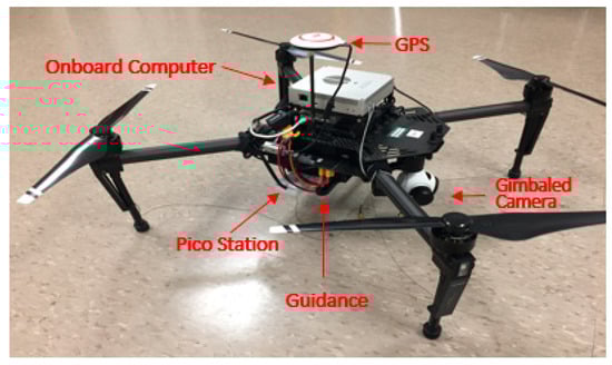
Figure 1.
DJI M100 quadcopter. Pico Station is the wireless transmitter. Guidance module is used for height measurements.
The mobile landing platform used in this work is equipped with an embedded system interfaced with a GPS receiver, an IMU, and a Wi-Fi module that can transmit the position and velocity of the landing platform to the UAV at 10 Hz. The visual marker used is a matrix barcode (An “AprilTag” to be specific) shown in Figure 2. The AprilTag is mounted on the landing platform for visual tracking of the landing platform by the UAV. We have adopted a Robot Operating System (ROS) software package that provides an ROS wrapper for the AprilTag library, enabling us to obtain the position and orientation of the tag with respect to the camera. One of the advantages of using AprilTags in this work is to minimize the effort in object recognition for vision-based target tracking.
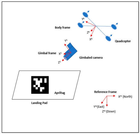
Figure 2.
System overview and main coordinate frames.
With the position of the target (or AprilTag) with respect to the camera position, we can easily obtain the desired gimbal angle for the camera to point at the target. In other words, we always want to have the target at the center of the image plane captured by the camera to minimize the probability of target loss. The desired gimbal angle can be obtained by
where and are, respectively, the desired pitch and yaw angle of the gimbal; and are, respectively, the current pitch and yaw angle of the gimbal; and are, respectively, the lateral and longitudinal position of the target on the image plane coordinates; and is the distance between the target and the camera. Since the roll of the gimbal is only ±15 degrees, we do not use it for target tracking. The desired gimbal angles are computed every time an AprilTag is detected (~30 Hz) and sent to a proportional derivative (PD) controller for the gimbaled camera to track the landing platform in a timely fashion.
4. Modeling
4.1. Dynamic Model
The dynamic model of the UAV used in this work can be given by [18]
where is the mass of the UAV, is the acceleration of the UAV, is the nominal acceleration, is the rotation matrix from the north-east-down (NED) reference frame to the body frame, T is the total thrust generated by the UAV rotors, and is the air damping force. Here, is given by
with the shorthand notation and . The angular positions denote, respectively, the roll, pitch, and yaw angles of the UAV. Thus, (2) can be written as
where , , and represent the position in north, east, and down, respectively; their first and second derivatives are, respectively, velocities and accelerations; and is the friction coefficient with which the air damping force is roughly modeled as a proportional signed quadratic velocity. Note that the inputs to the UAV are thrust (T), roll (), pitch (), and yaw in this model.
The longitudinal motion in the pitch plane is regulated by a PD controller to maintain (nearly) constant flight altitude, i.e., and . By applying the thrust of and assuming = 0 for constant altitude, we can simplify (4) by
Since the dynamics of the UAV in this work stays near the equilibrium point () without any aggressive maneuvers, we can linearize (5) at the equilibrium point to obtain
which can be written as
We have now a state space representation of the linearized system given by
where is the input to the system.
4.2. Kalman Filter for Landing Platform Position Estimation
At the beginning of autonomous landing tasks, our target localization algorithm relies on the position and velocity data transmitted from the landing platform. At this stage, the position data are measured by the GPS receiver integrated with the landing platform. As the UAV approaches the landing platform, the UAV still relies on the GPS data until the distance between the UAV and the landing platform is close enough for the landing platform to be observed by the onboard gimbaled camera.
To localize the landing platform at this stage, a gimbaled camera on-board the UAV is used to calculate the relative position of an AprilTag on the landing platform. This measurement occurs on a frame-by-frame basis with some noise. We have formulated a Kalman filter to optimally estimate and predict the location of the mobile landing platform as follows
where is the state vector at time ; is the sensor measurements; is the state transition matrix, representing the kinematic motion of the landing platform in the discrete time domain; is the observation matrix; is a zero mean Gaussian random vector with covariance , representing system uncertainty; and is a zero mean Gaussian random vector with covariance , representing sensor noise. The state vector is defined by , where are, respectively, the north and east position of the landing platform and are, respectively, the north and east velocity of the landing platform. The state transition matrix is given by
where is the time step. The observation matrix is the identity matrix, since we can directly measure all state variables.
In our implementation of Kalman filter, we have used a linear kinematic model for the mobile landing platform because we assume that the landing platform, as a cooperative agent in this application, travels in a linear path or a slightly curved path without any aggressive motion so that the UAV can easily land on the platform. It is well known that Kalman filters are the optimal state estimator for systems with linear process and measurement models and with additive Gaussian uncertainties whereas common KF variants, such as extended Kalman filter (EKF) and unscented Kalman filter (UKF), take linearization errors into account to improve the estimation performance for nonlinear systems. It is important to note that there is no theoretical guarantee of optimality in EKF and UKF whereas it has been proved that KF is an optimal state estimator [30]. In other words, an EKF and UKF are extensions of KF that can be applied to nonlinear systems to mitigate linearization error at the cost of losing optimality. Although EKF and UKF outperform linear KF for nonlinear systems in most cases, in our application, EKF or UKF is not necessary or they can potentially degrade the performance of linear state estimates.
4.3. Model Predictive Control of UAV
At an experimental level and as investigated in detail in [31], linear MPC and nonlinear MPC for control of rotary wing micro aerial vehicles have more or less the same performance in the case of non-aggressive maneuvers even in the presence of disturbances. In particular, in hovering conditions or for step response tracking, the performance of linear MPC and nonlinear MPC are very close to each other. However, in the case of aggressive maneuvers, nonlinear MPC outperforms linear MPC. This is due to the fact that nonlinear MPC accounts for the nonlinear effects in the whole dynamic regime of a micro aerial vehicle. In this work, we have employed a linear MPC scheme for achieving non-aggressive trajectory tracking and as is demonstrated in [31], the performance of linear MPC schemes are very close to the performance of nonlinear MPC schemes in these operating conditions. Furthermore, at a theoretical level and as demonstrated in [32], nonlinear MPC is reduced to linear MPC under certain conditions. In particular, when sequential quadratic programming (SQP) is deployed on NMPC, and the reference trajectory is used as an initial guess, the first step of a full-step Gauss–Newton SQP delivers the same control solution as a linear MPC scheme (see Lemma 3.1 in [32]). Since the target is moving on a path that is described by a straight line, and since the center of mass of the drone is moving on an approximate straight line, while the drone is maintaining an almost constant orientation; the dynamics of the drone evolve in a limited range where using a linear MPC scheme is justified.
To apply MPC to the dynamic system given in (7), we have discretized the system with the time step of s. In the remainder of the paper, refers only to the discrete time state, i.e., .
Then, the prediction with the future system inputs can be given by
where is the -step prediction of the state at time with . Then, the augmented state predictions can be given by
This equation can be written in a condensed form:
The future system inputs can be calculated by the optimal solution of the following cost function with constraints using the batch approach and quadratic programming [33].
where is the reference state of the desired trajectory; Q and R are the weight matrices for states and inputs, respectively; and is the weighting factor between the state cost and the input energy cost; is the velocity in north; is the velocity in east; is the desired pitch angle; is the desired roll angle; is the maximum UAV speed; and is the maximum tilt angle (roll and pitch) of the UAV. In this study, we used m/s and .
Substituting in (13) into (14) yields
where selects all velocity estimations from , that is
5. Simulation Results
To validate our control method for autonomous landing on a moving platform, we used the DJI hardware-in-the-loop (HITL) simulation environment. As shown in Figure 3a, the control panel of the HITL provides the initial settings for flight simulations as well as wind disturbances.
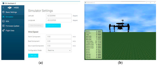
Figure 3.
HITL simulation provided by DJI. (a) Control panel, in which acceleration, velocity, position, and attitude information are provided; (b) simulator panel.
5.1. Localization the Landing Platform
At the beginning of autonomous landing tasks, our target localization algorithm relies on the position and velocity data transmitted from the landing platform. At this stage, the position data are measured by the GPS receiver integrated with the landing platform. As the UAV approaches the landing platform, the UAV still relies on the GPS data until the distance between the UAV and the landing platform is close enough for the landing platform to be observed by the camera. At this stage, we use the distance measurements from the AprilTag detection algorithm. A video stream obtained from the camera is processed at a ROS at 30 Hz to obtain the position of the AprilTag in the camera frame. Then, we calculate the position of the AprilTag in the reference frame.
In order to validate the performance of the Kalman filter, we introduced additive white Gaussian noise (AWGN), with its standard deviation of 0.03 () in the position measurements to simulate the measurement error from the Apriltag detection and of 0.18 () in the velocity measurements to simulate the velocity measurement error. We found these sensor noises empirically.
The measurement noise covariance matrix for the Kalman filter is given by
where , , , and are the variances of sensor noise of the lateral position, longitudinal position, lateral velocity, and longitudinal velocity, respectively. So, we set and . The state transition covariance matrix is given by
where is the time step and is the estimated variance of the acceleration of the landing platform. In this work, we have 0.025 s and . Figure 4 shows the estimated position and velocity of the landing platform obtained from the Kalman filter. The root mean square (RMS) errors are 7.97 cm for the position and 0.0336 m/s for the velocity of the landing platform, which are satisfactory for a 1.15m wingspan quadcopter to land on it.
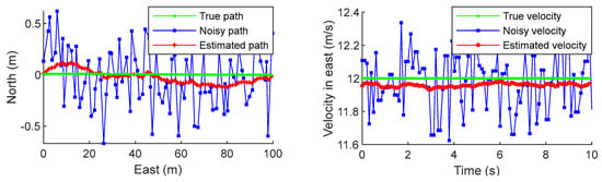
Figure 4.
Position & velocity noisy data and estimated data.
The startup situations are all the same: the target starts at 50 m in the north from the origin and moves toward east with constant 12 m/s speed, and at the same time, the UAV starts at the origin with zero initial speed. The UAV first enters the approach state and tracks the target until the UAV is on the top of target, and then enters the landing state and starts to land on the target.
5.2. Selection of MPC Parameters
For this study, we set for the prediction horizon and for the control horizon, with a sampling time of 0.025 s. Consequently, for every time step, the MPC optimizes the flight trajectory of the UAV for the next 0.3 s. For the state weight matrix Q, the weights for both the longitudinal and the lateral positions are set to 10 for the first seven prediction steps out of 12 steps, the weights for both the longitudinal and the lateral velocities are set to 1.5 for the last five prediction steps, and all the rest are set to 1. For the input weight matrix R, we simply set it to the identity matrix. The mass of the UAV is 2.883 kg.
5.3. Straight Path without Wind Disturbance
We have tested our method with various speeds set for the landing platform. In this experiment, we assume that the sensor outputs have been contaminated by noise, and therefore the estimates of the target location are obtained through the Kalman filter discussed in Section 5.1. Figure 5 demonstrates the performance of the MPC for approaching and landing on the platform traveling at the speeds of 4 m/s, 8 m/s, and 12 m/s. The trajectories of the UAV following and landing on the platform travelling on a straight path are shown in Figure 5a. It is apparent that it takes more time for the UAV flying at 12 m/s to approach and land on the target than for the UAV flying at 4 m/s performing the same task. Figure 5b shows in 3D that the UAV has landed on the landing platform moving at 12 m/s on a straight path. Figure 5c,d show the position in north and east of the UAV along with the measured location of the landing platform. As shown in Figure 5e, the UAV maintains the altitude while it is approaching the landing platform and if the distance between the UAV and the landing platform becomes less than 1 m, the UAV starts descending. Figure 5f shows the distance between the UAV and the landing platform. In these simulations, we have used the vertical distance between the UAV and the landing platform to decide if the UAV has landed (DJI Guidance discussed in Section 3 can provide this quantity in flight experiments).
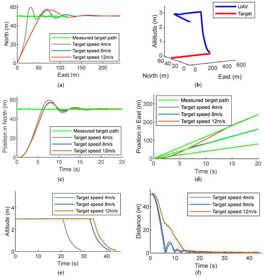
Figure 5.
The UAV autonomously landing on a target moving on a straight path with noisy measurements, when target speed varies among 4 m/s, 8 m/s, and 12 m/s. (a) Top-down view; (b) 3D plot (target speed 12 m/s); (c) position in the north; (d) position in the east; (e) altitude; (f) 2D distance error.
Table 1 summarizes the performance for the three different speeds of the landing platform with and without measurement noise. As the speed of the landing platform increases, the approach time, landing time, and landing error also increase. For the noisy measurements of the platform position and velocity, the UAV demonstrates similar approach time and landing time as the no noise case. The largest landing error with noisy measurements is 26 cm from the center of the landing platform, which shows that the method proposed in this work can be considered as a viable solution for autonomous landing on a moving platform.

Table 1.
Performance of autonomous landing on a target travelling on a straight path at various speeds.
5.4. Straight Path with Wind Disturbance
To validate the robustness of our method under wind disturbances, we implemented an integral controller that can be seamlessly fused with the MPC. We conducted simulations with a wind speed of 5 m/s and a target speed of 8 m/s. The integral controller is designed to accumulate the position error to fight against the wind. Figure 6 shows that the UAV reaches the desired position in approximately 9 s with zero steady-state error when the integral constant of . If is too small (e.g., ), the UAV cannot reach the desired target position, with a steady-state error of approximately 1.6 m. For a large value of (e.g., ), the closed-loop system becomes unstable as shown in Figure 6b.
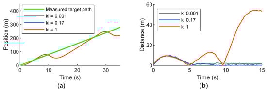
Figure 6.
System response: (a) integrator ramp response; (b) distance error between UAV and target of integrator ramp response.
Figure 7a shows the trajectories of the UAV following and landing on the platform travelling on a straight path in the presence of a wind disturbance with a constant speed of 5 m/s. Since the UAV in this work can fly at a speed of up to 18 m/s, the maximum target speed we set in the simulations is 12 m/s for a headwind speed of 5 m/s. Figure 7b–d shows the measured location of the landing platform and the trajectories of the UAV in no wind, a 5 m/s tailwind and a 5 m/s headwind. It is apparent that a tailwind has minimal effect on approach time, landing time, and landing error, while a headwind makes the UAV slow down. As shown in Figure 7e,f, it is evident that the approach time dramatically increases with a headwind.
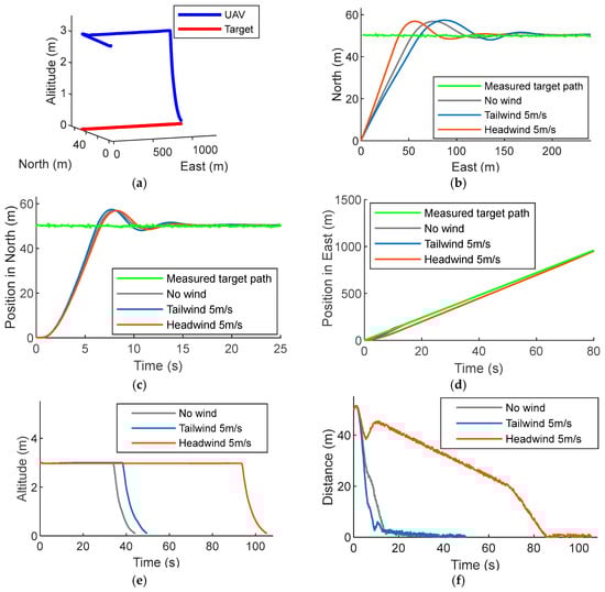
Figure 7.
The UAV autonomously landing on a 12 m/s target moving on a straight path, under the condition of measurement noise and east wind disturbance. (a) 3D plot (west wind 5 m/s); (b) top-down view; (c) position in the north; (d) position in the east; (e) altitude; (f) horizontal distance error.
Table 2 summarizes the simulation results under the presence of wind disturbances. The approach time and landing time in the presence of a headwind disturbance are much greater than those in the presence of no wind or a tailwind. However, the landing error with a headwind is just slightly larger than the error with no wind. In case of noisy measurements, the landing error is still bounded by 37 cm, which shows that the method proposed in this work is robust enough for wind disturbances and noisy sensor measurements.
Table 2.
Performance of autonomous landing on 12 m/s straightly moving target with varying wind speed.
5.5. Curved Path
We also conducted simulations with the landing platform travelling on a curved path. Figure 8a shows the UAV lading on a platform moving at 8 m/s on a curved path with a radius of 300 m. It is shown in Figure 8b,c that it takes approximately 43 s for the UAV to approach the platform. Figure 8e,f show that it takes an additional 9 s to land on the target, with a 35-cm error, which demonstrates that the proposed method is a viable solution for a landing platform traveling on a curved path as well as a straight path.
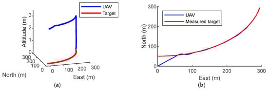
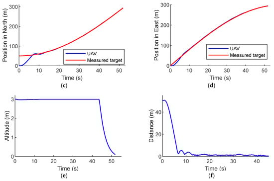
Figure 8.
The UAV autonomously landing on a 12 m/s circularly moving target with noisy measurements. (a) 3D plot; (b) top-down view; (c) position in the north; (d) position in the east; (e) altitude; (f) horizontal distance error.
6. Conclusions and Future Work
In this work, we propose a new control method that allows a micro UAV to land autonomously on a moving platform in the presence of uncertainties and disturbances. Our main focus with this control method lies in the implementation of such an algorithm in a low-cost, lightweight embedded system that can be integrated into micro UAVs. We have presented our approach, consisting of vision-based target following, optimal target localization, and model predictive control, for optimal guidance of the UAV. The simulation results demonstrate the efficiency and robustness with wind disturbances and noisy measurements.
In the future, we aim to conduct flight experiments to validate the control methods we present in this paper. The landing platform can be a flat surface with a dimension of at least m for safe landing and it will be mounted on a vehicle (for example, a truck bed or a flat root of a golf cart). We will also develop robust recovery methods that can save the vehicle from various failures, such as communication loss between the UAV and the landing platform, that can occasionally occur in the real world.
Author Contributions
Conceptualization, Y.F., C.Z., and S.B.; Methodology, Y.F.; Software, Y.F. and C.Z.; Validation, Y.F. and C.Z.; Formal Analysis, Y.F. and C.Z.; A.M and S.B.; Visualization, Y.F.; Supervision, S.R., A.M., and S.B.; Project Administration, S.B.; Funding Acquisition, S.B.
Funding
This research was funded by a University of Michigan-Dearborn Research Initiation Seed Grant (grant number: U051383).
Conflicts of Interest
The authors declare no conflict of interest.
References
- Cherubini, A.; Papini, A.; Vertechy, R.; Fontana, M. Airborne Wind Energy Systems: A review of the technologies. Renew. Sustain. Energy Rev. 2015, 51, 1461–1476. [Google Scholar] [CrossRef]
- Williams, A. Persistent Mobile Aerial Surveillance Platform using Intelligent Battery Health Management and Drone Swapping. In Proceedings of the 2018 4th International Conference on Control, Automation and Robotics (ICCAR), Auckland, New Zealand, 20–23 April 2018; pp. 237–246. [Google Scholar]
- Sri, K.R.B.; Aneesh, P.; Bhanu, K.; Natarajan, M. Design analysis of solar-powered unmanned aerial vehicle. J. Aerosp. Technol. Manag. 2016, 8, 397–407. [Google Scholar] [CrossRef]
- Guedim, Z. Hydrogen-Powered Drone ‘Hycopter’ Stays in Flight for 4 Hours. 2018. Available online: Edgylabs.com/hydrogen-powered-drone-hycopter-flight-4-hours (accessed on 1 August 2018).
- Garone, E.; Determe, J.-F.; Naldi, R. Generalized Traveling Salesman Problem for Carrier-Vehicle Systems. J. Guid Control Dyn. 2014, 37, 766–774. [Google Scholar] [CrossRef]
- Wenzel, K.E.; Masselli, A.; Zell, A. Automatic Take Off, Tracking and Landing of a Miniature UAV on a Moving Carrier Vehicle. J. Intell. Robot. Syst. 2011, 61, 1–7. [Google Scholar] [CrossRef]
- Venugopalan, T.K.; Taher, T.; Barbastathis, G. Autonomous landing of an Unmanned Aerial Vehicle on an autonomous marine vehicle. In Proceedings of the 2012 OCEANS, Hampton Roads, VA, USA, 14–19 October 2012; pp. 1–9. [Google Scholar]
- Coutard, L.; Chaumette, F. Visual detection and 3D model-based tracking for landing on an aircraft carrier. In Proceedings of the IEEE International Conference on Robotics and Automation, Shanghai, China, 9–13 May 2011; pp. 1746–1751. [Google Scholar]
- Coutard, L.; Chaumette, F.; Pflimlin, J.M. Automatic landing on aircraft carrier by visual servoing. In Proceedings of the IEEE International Conference on Intelligent Robots and Systems, San Francisco, CA, USA, 25–30 September 2011; pp. 2843–2848. [Google Scholar]
- Yakimenko, O.A.; Kaminer, I.I.; Lentz, W.J.; Ghyzel, P.A. Unmanned aircraft navigation for shipboard landing using infrared vision. IEEE Trans. Aerosp. Electron. Syst. 2002, 38, 1181–1200. [Google Scholar] [CrossRef]
- Erginer, B.; Altug, E. Modeling and PD Control of a Quadrotor VTOL Vehicle. In Proceedings of the 2007 IEEE Intelligent Vehicles Symposium, Istanbul, Turkey, 13–15 June 2007; pp. 894–899. [Google Scholar]
- Voos, H.; Nourghassemi, B. Nonlinear Control of Stabilized Flight and Landing for Quadrotor UAVs. In Proceedings of the 7th Workshop on Advanced Control and Diagnosis ACD, Zielo Gora, Poland, 17–18 November 2009; pp. 1–6. [Google Scholar]
- Ahmed, B.; Pota, H.R. Backstepping-based landing control of a RUAV using tether incorporating flapping correction dynamics. In Proceedings of the 2008 American Control Conference, Seattle, WA, USA, 11–13 June 2008; pp. 2728–2733. [Google Scholar]
- Shue, S.-P.; Agarwal, R.K. Design of Automatic Landing Systems Using Mixed H/H Control. J. Guid Control Dyn. 1999, 22, 103–114. [Google Scholar] [CrossRef]
- Wang, R.; Zhou, Z.; Shen, Y. Flying-wing UAV landing control and simulation based on mixed H2/H∞. In Proceedings of the 2007 IEEE International Conference on Mechatronics and Automation, ICMA 2007, Harbin, China, 5–8 August 2007; pp. 1523–1528. [Google Scholar]
- Lee, D.; Ryan, T.; Kim, H.J. Autonomous landing of a VTOL UAV on a moving platform using image-based visual servoing. In Proceedings of the IEEE International Conference on Robotics and Automation (ICRA), Saint Paul, MN, USA, 14–18 May 2012; pp. 971–976. [Google Scholar]
- Serra, P.; Cunha, R.; Hamel, T.; Cabecinhas, D.; Silvestre, C. Landing of a Quadrotor on a Moving Target Using Dynamic Image-Based Visual Servo Control. IEEE Trans. Robot. 2016, 32, 1524–1535. [Google Scholar] [CrossRef]
- Borowczyk, A.; Nguyen, D.-T.; Nguyen, A.P.-V.; Nguyen, D.Q.; Saussié, D.; le Ny, J. Autonomous Landing of a Multirotor Micro Air Vehicle on a High Velocity Ground Vehicle. J. Guid Dyn. 2016, 40, 2373–2380. [Google Scholar]
- Olson, E. AprilTag: A robust and flexible visual fiducial system. In Proceedings of the IEEE International Conference on Robotics and Automation, Shanghai, China, 9–13 May 2011; pp. 3400–3407. [Google Scholar]
- Beul, M.; Houben, S.; Nieuwenhuisen, M.; Behnke, S. Landing on a Moving Target Using an Autonomous Helicopter. In Proceedings of the 2017 European Conference on Mobile Robots (ECMR), Paris, France, 6–8 September 2017; pp. 277–286. [Google Scholar]
- Polvara, R.; Patacchiola, M.; Wan, J.; Manning, A.; Sutton, R.; Cangelosi, A. Toward End-to-End Control for UAV Autonomous Landing via Deep Reinforcement Learning. In Proceedings of the 2018 International Conference on Unmanned Aircraft Systems (ICUAS), Dallas, TX, USA, 12–15 June 2018; pp. 115–123. [Google Scholar]
- Juang, J.; Chien, L.; Lin, F. Automatic Landing Control System Design Using Adaptive Neural Network and Its Hardware Realization. IEEE Syst. J. 2011, 5, 266–277. [Google Scholar] [CrossRef]
- Lungu, R.; Lungu, M. Automatic landing system using neural networks and radio-technical subsystems. Chin. J. Aeronaut. 2017, 30, 399–411. [Google Scholar] [CrossRef]
- Qing, Z.; Zhu, M.; Wu, Z. Adaptive Neural Network Control for a Quadrotor Landing on a Moving Vehicle. In Proceedings of the 2018 Chinese Control And Decision Conference (CCDC), Shenyang, China, 9–11 June 2018; pp. 28–33. [Google Scholar]
- Lee, S.; Shim, T.; Kim, S.; Park, J.; Hong, K.; Bang, H. Vision-Based Autonomous Landing of a Multi- Copter Unmanned Aerial Vehicle using Reinforcement Learning. In Proceedings of the 2018 International Conference on Unmanned Aircraft Systems (ICUAS), Dallas, TX, USA, 12–15 June 2018; pp. 108–114. [Google Scholar]
- Templeton, T.; Shim, D.H.; Geyer, C.; Sastry, S.S. Autonomous vision-based landing and terrain mapping using an MPC-controlled unmanned rotorcraft. In Proceedings of the IEEE International Conference on Robotics and Automation, Roma, Italy, 10–14 April 2007; pp. 1349–1356. [Google Scholar]
- Wu, Y.; Qu, X. Obstacle avoidance and path planning for carrier aircraft launching. Chin. J. Aeronaut. 2015, 28, 695–703. [Google Scholar] [CrossRef]
- Samal, M.K.; Anavatti, S.; Garratt, M. Neural Network Based Model Predictive Controller for Simplified Heave Model of an Unmanned Helicopter. In Proceedings of the International Conference on Swarm, Evolutionary, and Memetic Computing, Bhubaneswar, India, 20–22 December 2012; pp. 356–363. [Google Scholar]
- Tian, J.; Zheng, Y.; Zhu, H.; Shen, L. A MPC and Genetic Algorithm Based Approach for Multiple UAVs Cooperative Search. In Proceedings of the International Conference on Computational and Information Science, Shanghai, China, 16–18 December 2005; pp. 399–404. [Google Scholar]
- Kalman, R.E. A New Approach to Linear Filtering and Prediction Problems 1. J. Basic Eng. 1960, 82, 35–45. [Google Scholar] [CrossRef]
- Kamel, M.; Burri, M.; Siegwart, R. Linear vs Nonlinear MPC for Trajectory Tracking Applied to Rotary Wing Micro Aerial Vehicles. IFAC 2017, 50, 3463–3469. [Google Scholar] [CrossRef]
- Gros, S.; Zanon, M.; Quirynen, R.; Bemporad, A.; Diehl, M. From linear to nonlinear MPC: Bridging the gap via the real-time iteration. Int. J. Control 2016, 7179, 1–19. [Google Scholar] [CrossRef]
- Francesco, B.; Alberto, B.; Manfred, M. Predictive Control for Linear and Hybrid Systems; Cambridge University Publisher: Cambridege, UK, 2017. [Google Scholar]
© 2018 by the authors. Licensee MDPI, Basel, Switzerland. This article is an open access article distributed under the terms and conditions of the Creative Commons Attribution (CC BY) license (http://creativecommons.org/licenses/by/4.0/).