Adaptive Control for UAV Landing on Moving Vehicles

Highlights

What are the main findings?

• A nonlinear adaptive control architecture combining backstepping control, super–twisting sliding modes, and adaptive internal model regulation was developed for autonomous UAV landing on moving vehicles subjected to unknown multi–frequency vertical oscillations.
• Simulation results demonstrated that the adaptive internal model regulator achieved smaller altitude tracking errors than the robust super–twisting sliding-mode controller, particularly under high-frequency platform oscillations.

What are the implications of the main findings?

• Adaptive internal model regulation constitutes a viable alternative for autonomous UAV landing under uncertain oscillatory platform dynamics, particularly when the disturbance frequencies are unknown.
• The obtained results indicate that adaptive internal model regulation can be effectively applied to autonomous UAV landing problems involving unknown multi-frequency platform oscillations.

Abstract

This paper addresses the problem of autonomous landing of a quadrotor unmanned aerial vehicle (UAV) on a moving ground vehicle subjected to unknown vertical oscillations generated by road irregularities. The proposed approach considers simultaneous longitudinal, lateral, heading, and altitude regulation in the presence of nonlinear coupled dynamics, aerodynamic effects, and platform motion disturbances. A nonlinear control architecture is developed by combining backstepping techniques, super-twisting sliding-mode control, and an adaptive internal model regulator. The longitudinal, lateral, and heading subsystems are stabilized through a block backstepping–sliding-mode framework, whereas the altitude subsystem is regulated using an adaptive internal model controller capable of compensating unknown multi-frequency oscillatory disturbances without prior knowledge of their amplitudes or frequencies. The complete UAV dynamics are derived from the Newton–Euler formulation, including aerodynamic forces, gyroscopic effects, and coupled translational–rotational dynamics. To improve robustness and avoid algebraic differentiation, exact first-order differentiators based on the super-twisting algorithm are incorporated into the control implementation. The proposed adaptive regulator is compared against a robust super-twisting sliding-mode altitude controller under low- and high-frequency oscillatory platform motions. Simulation results demonstrate that the adaptive internal model regulator achieves accurate trajectory tracking and consistently lower accumulated tracking errors than the robust super-twisting sliding-mode controller under both low- and high-frequency platform oscillations. These results highlight the suitability of adaptive output regulation techniques for autonomous UAV landing operations under oscillatory platform conditions with measurement noise.

1. Introduction

Autonomous Unmanned Aerial Vehicles (UAVs) have become an important research area within the aerospace industry due to their increasing range of civilian and military applications. Their ability to perform tasks without exposing human operators to hazardous environments has enabled their use in surveillance, infrastructure inspection, precision agriculture, environmental monitoring, search and rescue, medical supply delivery, and defense operations.

A key challenge in UAV technology is the development of reliable autonomous flight algorithms that enable aircraft to execute missions safely and without human intervention. Such algorithms must guarantee accurate navigation and control throughout all phases of flight, including take-off, cruise, and landing. Among these phases, landing is particularly critical because it requires precise regulation of the vehicle’s position, velocity, and attitude. Even under favorable operating conditions, landing remains one of the most demanding flight maneuvers and is a major source of accidents, requiring high levels of precision and robustness [1]. Consequently, the development of autonomous landing systems has received considerable attention, especially for landing on moving platforms, where the relative motion between the UAV and the platform significantly increases the complexity of the control problem.

Numerous approaches have been proposed for autonomous landing on moving platforms. Vision-based methods combined with conventional controllers have been widely investigated for platforms undergoing horizontal motion. Representative examples include the works in refs. [2,3,4,5,6,7,8], where different platform detection algorithms and control strategies were developed assuming negligible vertical platform motion. More challenging scenarios involving simultaneous horizontal and vertical motion have also been considered. In ref. [9], a color-based detection algorithm was combined with an L₁ adaptive controller for trajectory tracking of a moving vehicle. In ref. [10], autonomous landing on an unmanned surface vehicle was achieved using color- and shape-based target detection together with a PID controller. Likewise, ref. [11] addressed landing on a horizontally moving platform subject to unpredictable vertical oscillations by employing a Motion Capture (MoCap) system for position estimation and a PI controller with feedforward compensation.

More recently, optimization-based and learning-based control techniques have emerged as promising alternatives. Model Predictive Control (MPC) has been applied to autonomous landing because it explicitly incorporates system dynamics and operational constraints while optimizing future control actions. However, MPC relies on an accurate prediction model and requires solving an optimization problem online, which may limit its implementation on embedded UAV platforms with limited computational resources [12]. Deep Reinforcement Learning (DRL) has also attracted considerable interest because it can learn complex landing policies directly from interaction data without requiring an explicit mathematical model. Nevertheless, DRL methods typically require extensive training large datasets and often provide limited theoretical guarantees regarding stability, robustness, and safety [4,13].

Table 1. Qualitative comparison of representative autonomous landing approaches for moving platforms.

Reference	Control Method	Moving Platform	Vertical Oscillations	Online Optimization	Stability Analysis	Computational Demand
Hanseob [9]	L1 Adaptive Control	✓	✓	×	Partial	Moderate
Venugopalan [10]	PID	✓	✓	×	×	Low
Kesavan [12]	Model Predictive Control (MPC)	✓	✓	✓	✓	High
Xie [13]	Deep Reinforcement Learning (DRL)	✓	✓	×	×	High
This work	Adaptive Internal Model Regulator	✓	✓	×	✓	Low

summarizes the main characteristics of representative autonomous landing approaches reported in the literature. Unlike optimization-based and learning-based methods, the proposed adaptive internal model regulator does not require online optimization or offline training while preserving a rigorous nonlinear stability analysis. These characteristics make the proposed approach computationally attractive for autonomous landing on moving platforms subject to vertical oscillations.

In contrast to these approaches, this paper proposes an adaptive control strategy based on the Internal Model Principle. Rather than relying on online optimization or offline learning, the proposed controller exploits the periodic characteristics of the platform motion to achieve accurate trajectory tracking with low computational complexity while preserving rigorous stability properties derived from nonlinear control theory.

Specifically, this work considers the challenging problem of autonomous landing on a moving ground vehicle undergoing both horizontal motion and vertical multi-frequency oscillations. The landing maneuver is divided into two stages: vehicle tracking and final landing. The longitudinal, lateral, and yaw dynamics are controlled using a sliding-mode backstepping strategy, whereas the altitude dynamics are regulated using two alternative approaches. The first employs a robust super-twisting sliding-mode controller [14], while the second implements the Globally Adaptive Internal Model Regulator proposed in ref. [15]. A comparative evaluation demonstrates that the proposed adaptive internal model regulator achieves superior altitude tracking performance with reduced control effort, particularly under high-frequency platform oscillations, thereby providing an effective and computationally efficient alternative to robust sliding-mode control.

2. Mathematical Model

The dynamic behavior of the quadrotor Unmanned Aerial Vehicle (UAV) is represented by a six–degree-of-freedom rigid-body model derived from the Newton–Euler formalism. Two orthogonal reference frames are defined: the inertial (earth-fixed) frame $RC(O,e_1,e_2,e_3)$ and the body-fixed frame $R\Gamma (\Omega ,{\epsilon }_1,{\epsilon }_2,{\epsilon }_3)$, whose origin, $\Omega$, coincides with the UAV’s center of mass. Both frames follow the North–East–Down (NED) convention, where the third axis points toward the Earth.

The translational motion of the vehicle in the $RC$ frame is described by the position vector $p=\mathrm{col}(x,y,z)$, while its attitude is parameterized by the Euler angles $\alpha =\mathrm{col}(\varphi ,\theta ,\psi )$, corresponding to roll, pitch, and yaw, respectively. These angles are usually limited to the range $(-\pi /2,\pi /2)$ to avoid singularities. The linear and angular velocities expressed in the body frame are $v=\mathrm{col}(u,v,w)$ and $\omega =\mathrm{col}(p,q,r)$.

The orientation of the UAV with respect to the inertial frame is determined by the rotation matrix

$$\mathcal{R}\left(\alpha \right)=\left(\phantom{(}\begin{array}{ccc}{c}_{\psi }{c}_{\theta }& c_{\psi }{s}_{\theta }{s}_{\varphi }-s_{\psi }{c}_{\varphi }& c_{\psi }{s}_{\theta }{c}_{\varphi }+s_{\psi }{s}_{\varphi }\\ s_{\psi }{c}_{\theta }& s_{\psi }{s}_{\theta }{s}_{\varphi }+c_{\psi }{c}_{\varphi }& s_{\psi }{s}_{\theta }{c}_{\varphi }-c_{\psi }{s}_{\varphi }\\ -s_{\theta }& c_{\theta }{s}_{\varphi }& c_{\theta }{c}_{\varphi }\end{array}\phantom{)}\right)$$

(1)

where $s_{(·)}=sin(·)$ and $c_{(·)}=cos(·)$. This matrix transforms any vector expressed in the $R\Gamma$ frame into its representation in the $RC$ frame and provides the coupling between translational and rotational dynamics.

The angular velocity $\omega$ is related to the Euler angle rates $\dot{\alpha }$ through the kinematic transformation matrix

$$\omega =M\left(\alpha \right)\dot{\alpha },M\left(\alpha \right)=\left(\phantom{(}\begin{array}{ccc}1& 0& -s_{\theta }\\ 0& c_{\varphi }& c_{\theta }{s}_{\varphi }\\ 0& s_{\varphi }& c_{\theta }{c}_{\varphi }\end{array}\phantom{)}\right).$$

(2)

This transformation expresses how variations in the Euler angles generate body angular velocity components. For maneuvers with small roll and pitch angles—such as hover or steady landing phases—$M\left(\alpha \right)\approx I_{3\times 3}$, which simplifies subsequent derivations.

The vehicle mass is denoted by $m>0$, and the inertia tensor in the body frame is $J=\mathrm{diag}(J_x,J_y,J_z)$. To compactly express rotational coupling, the skew–symmetric operator associated with $\omega$ is introduced as

$$\tilde{\omega }=\left(\phantom{(}\begin{array}{ccc}0& -r& q\\ r& 0& -p\\ -q& p& 0\end{array}\phantom{(}\right),$$

(3)

which satisfies $\omega \times y=\tilde{\omega }y$ for any vector $y\in {\mathbb{R}}^3$.

Using these definitions, the UAV dynamics in the body–fixed frame $R\Gamma$ are expressed through the Newton–Euler equations:

$$m\dot{v}+\tilde{\omega }\left(mv\right)=F_{\mathrm{prop}}-F_{\mathrm{aero}}-F_{\mathrm{grav}},J\dot{\omega }+\tilde{\omega }\left(J\omega \right)=T_{\mathrm{prop}}-T_{\mathrm{aero}}-T_{\mathrm{gyro}}.$$

(4)

where $F_{\mathrm{prop}}$ and $T_{\mathrm{prop}}$ are the forces and moments produced by the propellers, respectively. $F_{\mathrm{grav}}$ is the gravitational force, $F_{\mathrm{aero}}$ and $T_{\mathrm{aero}}$ are the aerodynamic forces and moments acting on the UAV, respectively, and $T_{\mathrm{gyro}}$ defines the gyroscopic effects resulting from the propeller rotations. The first equation describes translational motion influenced by propulsive, aerodynamic, and gravitational forces, while the second governs rotational motion under propulsive, aerodynamic, and gyroscopic moments.

Each rotor $i\in \{1,2,3,4\}$ produces an upward thrust $F_i=b{\omega }_{p,i}^2\ge 0$, where $b>0$ is the thrust coefficient determined by blade geometry and air density, and ${\omega }_{p,i}$ is the rotor angular speed. The total propulsive force and torque acting on the vehicle are

$$F_{\mathrm{prop}}=\left(\phantom{(}\begin{array}{c}0\\ 0\\ {\sum }_{i=1}^4{F}_i\end{array}\phantom{(}\right),T_{\mathrm{prop}}=\left(\phantom{(}\begin{array}{c}d(F_4-F_2)\\ d(F_3-F_1)\\ c{\sum }_{i=1}^4{(-1)}^i{F}_i\end{array}\phantom{(}\right),$$

(5)

where d is the distance from the center of mass to each rotor and c is the drag factor associated with the aerodynamic resistance of the propellers.

The gravitational force, expressed in $RC$ as $mg{e}_3$ with $e_3={[0,0,1]}^T$, is transformed into the body frame as

$$F_{\mathrm{grav}}=\mathcal{R}{\left(\alpha \right)}^{\top }mG,G=\mathrm{col}(0,0,9.81){\mathrm{m}/\mathrm{s}}^2.$$

(6)

In addition to gravitational effects, aerodynamic forces and torques act on the UAV, opposing its translational and angular motion:

$$F_{\mathrm{aero}}=\mathrm{col}(A_u,A_v,A_w),T_{\mathrm{aero}}=\mathrm{col}(A_p,A_q,A_r),$$

(7)

where each aerodynamic component is modeled as

$$A_i=\frac{1}{2}\rho C_i{(\omega -{\omega }_{\mathrm{air}})}^2,i\in \{u,v,w,p,q,r\},$$

(8)

with $\rho$ denoting air density, $C_i$ aerodynamic coefficients, and $\omega -{\omega }_{\mathrm{air}}$ the relative velocity between the UAV and the surrounding airflow.

The gyroscopic coupling induced by the spinning rotors contributes an additional moment given by

$$T_{\mathrm{gyro}}={\displaystyle \sum _{i=1}^4}{(-1)}^{i+1}{J}_r\tilde{\omega }{e}_3{\omega }_{p,i},$$

(9)

where $J_r$ is the rotor polar moment of inertia and $e_3={[0,0,1]}^T$ is the unit vector along the body z-axis. This term accounts for cross-coupling effects between body angular motion and individual rotor spin.

By substituting these expressions into (4), the translational and rotational dynamics in the body frame are written explicitly as

$$\begin{array}{cc}\hfill \dot{v}& =-\tilde{\omega }v+{\displaystyle \frac{1}{m}}\left(F_{\mathrm{prop}}-F_{\mathrm{aero}}-F_{\mathrm{grav}}\right),\hfill \\ \hfill J\dot{\omega }& =-\tilde{\omega }\left(J\omega \right)+T_{\mathrm{prop}}-T_{\mathrm{aero}}-T_{\mathrm{gyro}}.\hfill \end{array}$$

(10)

Transforming the translational motion into the inertial frame $RC$ yields

$$\ddot{p}={\displaystyle \frac{1}{m}}\mathcal{R}\left(\alpha \right)\left(F_{\mathrm{prop}}-F_{\mathrm{aero}}\right)-G,$$

(11)

which explicitly couples the thrust direction to the attitude angles via $\mathcal{R}\left(\alpha \right)$.

For controller design and numerical simulation, the model is often expressed in a component-wise state-space form. Introducing the collective input vector $U=\mathrm{col}(U_1,U_2,U_3,U_4),$

$$\begin{array}{cc}\hfill U_1& =F_1+F_2+F_3+F_4,\hfill \\ \hfill U_2& =F_4-F_2,\hfill \\ \hfill U_3& =F_3-F_1,\hfill \\ \hfill U_4& =-F_1+F_2-F_3+F_4,\hfill \\ \hfill {\omega }_p& =-{\omega }_{p,1}+{\omega }_{p,2}-{\omega }_{p,3}+{\omega }_{p,4}\hfill \end{array}$$

(12)

and assuming small perturbations so that $M\left(\alpha \right)\approx I$ (i.e., $\dot{\alpha }\approx \omega$), the UAV dynamics reduce to the explicit acceleration form

$$\left(\phantom{(}\begin{array}{c}\ddot{\varphi }\\ \ddot{\theta }\\ \ddot{\psi }\\ \ddot{z}\\ \ddot{x}\\ \ddot{y}\end{array}\phantom{(}\right)=\left(\phantom{(}\begin{array}{c}\dot{\theta }\dot{\psi }{a}_1+\dot{\theta }{a}_2{\omega }_p+A_{\dot{\varphi }}+b_1{U}_2\\ \dot{\varphi }\dot{\psi }{a}_3+\dot{\varphi }{a}_4{\omega }_p+A_{\dot{\theta }}+b_2{U}_3\\ \dot{\theta }\dot{\varphi }{a}_5+A_{\dot{\psi }}+b_3{U}_4\\ A_z-g+{\displaystyle \frac{c_{\varphi }{c}_{\theta }}{m}}{U}_1\\ A_x+{\displaystyle \frac{U_1}{m}}(c_{\varphi }{s}_{\theta }{c}_{\psi }+s_{\varphi }{s}_{\psi })\\ A_y+{\displaystyle \frac{U_1}{m}}(c_{\varphi }{s}_{\theta }{s}_{\psi }-s_{\varphi }{c}_{\psi })\end{array}\phantom{(}\right).$$

(13)

The parameters $a_i$ and $b_i$ depend on the moments of inertia and the rotor geometry:

$$\begin{array}{cccccc}\hfill a_1& ={\displaystyle \frac{J_y-J_z}{J_x}},\hfill & \hfill a_2& =-{\displaystyle \frac{J_r}{J_x}},\hfill & \hfill b_1& ={\displaystyle \frac{d}{J_x}},\hfill \\ \hfill a_3& ={\displaystyle \frac{J_z-J_x}{J_y}},\hfill & \hfill a_4& =\phantom{-}{\displaystyle \frac{J_r}{J_y}},\hfill & \hfill b_2& ={\displaystyle \frac{d}{J_y}},\hfill \\ \hfill a_5& ={\displaystyle \frac{J_x-J_y}{J_z}},\hfill & \hfill & & \hfill b_3& ={\displaystyle \frac{1}{J_z}}.\hfill \end{array}$$

(14)

Aerodynamic effects can be compactly summarized by

$$\begin{array}{cc}\hfill A_F& ={\displaystyle \frac{1}{m}}\mathcal{R}\left(\alpha \right)F_{\mathrm{aero}}=\mathrm{col}(A_x,A_y,A_z),\hfill \\ \hfill A_T& =J^{-1}{T}_{\mathrm{aero}}=\mathrm{col}(A_{\dot{\varphi }},A_{\dot{\theta }},A_{\dot{\psi }}),\hfill \end{array}$$

(15)

which denote the translational and rotational aerodynamic contributions, respectively.

The complete model thus provides a fully coupled six-degree-of-freedom nonlinear representation of the quadrotor. It captures the combined influence of aerodynamic drag, gravitational load, propeller thrust, and gyroscopic coupling. This physically consistent formulation serves as a foundation for developing advanced control algorithms—particularly nonlinear and adaptive strategies—for stabilization and precision landing on moving platforms under realistic flight conditions.

3. Problem Statement

The problem of UAV control is addressed using the framework of output regulation, thereby forcing the system states $\left(xyz\psi \right)$ to asymptotically converge to the vehicle-generated reference trajectories $\begin{array}{cccccc}(& x_r& y_r& z_r& {\psi }_r& )\end{array}$.

Note that the translations depend on the angles, therefore the state-space model (13) can be rearranged as follows

3.1. Longitude

$$\begin{array}{cc}\hfill \ddot{x}& =A_x+{\displaystyle \frac{U_1}{m}}(c_{\varphi }{s}_{\theta }{c}_{\psi }+s_{\varphi }{s}_{\psi })\hfill \\ \hfill \ddot{\theta }& =\dot{\varphi }\dot{\psi }{a}_3+\dot{\varphi }{a}_4{\omega }_p+A_{\dot{\theta }}+b_2{U}_3\hfill \end{array}$$

(16)

3.2. Latitude

$$\begin{array}{cc}\hfill \ddot{y}& =A_y+{\displaystyle \frac{U_1}{m}}(c_{\varphi }{s}_{\theta }{s}_{\psi }-s_{\varphi }{c}_{\psi })\hfill \\ \hfill \ddot{\varphi }& =\dot{\theta }\dot{\psi }{a}_1+\dot{\theta }{a}_2{\omega }_p+A_{\dot{\varphi }}+b_1{U}_2\hfill \end{array}$$

(17)

3.3. Heading

$$\begin{array}{cc}\hfill \ddot{\psi }& =\dot{\theta }\dot{\varphi }{a}_5+A_{\dot{\psi }}+b_3{U}_4\hfill \end{array}$$

(18)

3.4. Altitude

$$\begin{array}{cc}\hfill \ddot{z}& =A_z-g+{\displaystyle \frac{c_{\varphi }{c}_{\theta }}{m}}{U}_1\hfill \end{array}$$

(19)

The trajectory tracking problem is thus decomposed into separate subproblems for each subsystem: altitudinal, longitudinal, latitudinal, and heading. It can be noted that the aerodynamic moments $A_T=\mathrm{col}(A_{\dot{\varphi }},A_{\dot{\theta }},A_{\dot{\psi }})$ and aerodynamic force $A_z$ are matched disturbances, while the remaining aerodynamic forces, $A_x$ and $A_y$, are unmatched ones. In the following subsection, we propose a control system assuming the aerodynamic forces are known; then, a sliding-mode observer designed by ref. [16] will be used to estimate these variables.

4. Review of Basic Facts on Regulator Theory

Consider a linear system subject to perturbation given by

$$\begin{array}{cc}\hfill \dot{x}& =Ax+Bu+\overline{D}d\hfill \end{array}$$

(20)

$$\begin{array}{cc}\hfill e& =Cx+\overline{Q}d\hfill \end{array}$$

(21)

where $x\in {\mathbb{R}}^n$ is the state, $u\in \mathbb{R}$ is the input, $d\in {\mathbb{R}}^{k+1}$ is the so-called extended disturbance, composed of disturbance and reference signal, and $e\in \mathbb{R}$ is the tracking error between the plant output $Cx$ and a reference signal $-\overline{Q}d$. The matrices $A\in {\mathbb{R}}^{n\times n}$, $B,C^T\in {\mathbb{R}}^{n\times 1}$, $\overline{D}\in {\mathbb{R}}^{n\times (k+1)}$ and $\overline{Q}\in {\mathbb{R}}^{1\times (k+1)}$ may vary in some neighborhood of the ‘nominal matrices’ $(A_0,C_0,B_0,{\overline{D}}_0,{\overline{Q}}_0)$. We consider a vector d consisting of a constant signal, of magnitude $m_0$, and k sinusoidal signals of magnitude $m_j$, frequency ${\omega }_j$, and phase ${\phi }_j$, $j=1,\cdots ,k$,

$$\begin{array}{cccccc}d=(& m_0& m_{1}sin({\omega }_{1}t+{\phi }_1)& \cdots & m_{k}sin({\omega }_{k}t+{\phi }_k)& {)}^T\end{array}$$

where ${\omega }_i\ne {\omega }_j$ if $i\ne j$. For the subsequent analysis, these signals are assumed to be generated by the so-called exosystem [17].

$$\dot{w}=Sw$$

(22)

with $w\in {\mathbb{R}}^{2k+1}$,

$$\begin{array}{cc}S& =\left(\begin{array}{cccc}0& 0& 0& 0\\ 0& S_i& 0& 0\\ 0& 0& \ddots & 0\\ 0& 0& 0& S_k\end{array}\right)\in {\mathbb{R}}^{(2k+1)\times (2k+1)}\hfill \\ S_j& =\left(\begin{array}{cc}0& 1\\ -{\omega }_j^2& 0\end{array}\right),j=1,\cdots ,k\hfill \end{array}$$

Setting $d=\tilde{D}w$, $\tilde{D}\in {\mathbb{R}}^{(k+1)\times (2k+1)}$, $P=\overline{D}\tilde{D}\in {\mathbb{R}}^{n\times (2k+1)}$, $Q=\overline{Q}\tilde{D}\in {\mathbb{R}}^{1\times (2k+1)}$, the system (20)–(22) can be rewritten as

$$\begin{array}{cc}\hfill \dot{x}& =Ax+Bu+Pw\hfill \end{array}$$

(23)

$$\begin{array}{cc}\hfill \dot{w}& =Sw\hfill \end{array}$$

(24)

$$\begin{array}{cc}\hfill e& =Cx+Qw.\hfill \end{array}$$

(25)

The output regulation problem under error feedback [18] consists of designing a controller

$$\begin{array}{cc}\hfill \dot{\zeta }& =F\zeta +Ge,\hfill \\ \hfill u& =H\zeta ,\hfill \end{array}$$

with $\zeta \in {\mathbb{R}}^{\nu }$, such that

(S)

The equilibrium point $(x,w,\zeta )=(0,0,0)$ of the unforced system

$$\begin{array}{cc}\hfill \dot{x}& =Ax+BH\zeta ,\hfill \\ \hfill \dot{w}& =Sw,\hfill \\ \hfill \dot{\zeta }& =F\zeta +GCx,\hfill \\ \hfill e& =Cx+Qw,\hfill \end{array}$$

is exponentially stable.

(R)

For any initial condition of the closed-loop system

$$\begin{array}{cc}\hfill \dot{x}& =Ax+BH\zeta +Pw,\hfill \\ \hfill \dot{w}& =Sw,\hfill \\ \hfill \dot{\zeta }& =F\zeta +G(Cx+Qw),\hfill \end{array}$$

the solution satisfies ${\displaystyle \underset{t\to \infty }{lim}e\left(t\right)=0.}$

Classic assumptions of the robust regulation theory are as follows [17,19,20]

Assumption 1.

The pair $(A,B)$ is stabilizable and the pair $(A,C)$ is detectable;

Assumption 2.

The matrix S is neutrally stable, that is, all its eigenvalues are on the imaginary axis;

Assumption 3.

For every P, Q, there exist solutions $\Pi \in {\mathbb{R}}^{n\times (2k+1)}$ and $\Gamma \in {\mathbb{R}}^{1\times (2k\times 1)}$ to the Francis equations

$$\begin{array}{cc}\hfill \Pi S& =A\Pi +B\Gamma +P\hfill \\ \hfill 0& =C\Pi +Q.\hfill \end{array}$$

Following ref. [15], it is possible to construct an immersion of the signal $u_{\mathrm{ss}}=\Gamma w$ as follows. The characteristic polynomial of the matrix S has the following expression

$$p_S\left(\lambda \right)={\lambda }^{2k+1}+{\theta }_{2k-1}{\lambda }^{2k-1}+\cdots +{\theta }_3{\lambda }^3+{\theta }_1\lambda$$

where ${\theta }_{2j}=0$, $j=1,\cdots ,k$, whereas the odd coefficients are nonzero and given by

$${\theta }_1={\displaystyle \prod _{j=1}^k}{\omega }_j^2,\cdots ,{\theta }_{2k-1}={\displaystyle \sum _{j=1}^k}{\omega }_j^2.$$

Hence, defining

$$\begin{array}{cc}\hfill z_0& =\Gamma w\hfill \\ & ⋮\hfill \\ \hfill {\dot{z}}_i& =z_{i+1}=\Gamma S^{i}w,i=0,1,\cdots ,2k-1\hfill \\ & ⋮\hfill \\ \hfill {\dot{z}}_{2k}& =-{\theta }_1{z}_1-\cdots -{\theta }_{2k-1}{z}_{2k-1}\hfill \end{array}$$

one gets that $u_{\mathrm{ss}}=Hz$, where $H=(\phantom{(}1 0 \cdots 0)$ $\in {\mathbb{R}}^{1\times (2k\times 1)}$.

Finally, using the transformation $\tilde{x}=x-\Pi w$, the interconnected system (23)–(25) can be transformed into

$$\begin{array}{cc}\hfill \dot{\tilde{x}}& =A\tilde{x}+B(u-Hz)\hfill \end{array}$$

(26)

$$\begin{array}{cc}\hfill \dot{z}& =\Phi \left(\theta \right)z\hfill \end{array}$$

(27)

$$\begin{array}{cc}\hfill e& =C\tilde{x}\hfill \end{array}$$

(28)

where

$$\begin{array}{ccc}\hfill \Phi \left(\theta \right)& =\hfill & \left(\begin{array}{cc}0& I_{2k\times 2k}\\ 0& \overline{\theta }\end{array}\right)\in {\mathbb{R}}^{(2k+1)\times (2k+1)}\hfill \\ \hfill \overline{\theta }& =\hfill & \left(\begin{array}{ccccccc}{\theta }_1& 0& {\theta }_3& 0& \cdots & {\theta }_{2k-1}& 0\end{array}\right).\hfill \end{array}$$

When the frequencies ${\omega }_j$, $j=1,\cdots k$, are unknown, and therefore the parameters ${\theta }_{2j-1}$, $j=1,\cdots k$, are also unknown, the regulation problem can be solved using the technique proposed in ref. [15]. Assuming that, for any $\theta \in {\mathbb{R}}^{2k}$, there exist matrices $\Pi \left(\theta \right)$, $\Sigma \left(\theta \right)$ solving the equations

$$\begin{array}{cc}\hfill \Pi \left(\theta \right)S& =A\Pi \left(\theta \right)+B\tilde{H}\Sigma \left(\theta \right)+P\hfill \end{array}$$

(29)

$$\begin{array}{cc}\hfill \Sigma \left(\theta \right)S& =F\Sigma \left(\theta \right)\hfill \end{array}$$

(30)

$$\begin{array}{cc}\hfill 0& =C\Pi \left(\theta \right)+Q\hfill \end{array}$$

(31)

then the controller

$$\begin{array}{cc}\hfill {\dot{\zeta }}_1& =(A_0-{\overline{G}}_1{C}_0){\zeta }_1+B_{0}u+{\overline{G}}_{1}e\hfill \\ \hfill {\dot{\zeta }}_2& =-{\overline{G}}_2{C}_0{\zeta }_1+(\Phi \left(\widehat{\theta }\right)-{\overline{G}}_2\mu ){\zeta }_2+{\overline{G}}_{2}e\hfill \\ \hfill \dot{\widehat{\theta }}& =-\Lambda {\overline{\zeta }}_2(e-C_0{\zeta }_1-\mu {\zeta }_2)\hfill \\ \hfill u& =K{\zeta }_1+{\phi }^T\left(\widehat{\theta }\right){\zeta }_2\hfill \end{array}$$

(32)

solves the Robust Output Regulation Problem, where K, ${\overline{G}}_1$ are such that $A_0+B_{0}K$, $A_0-{\overline{G}}_1{C}_0$ are Hurwitz, $\Lambda =\mathrm{diag}\{{\varrho }_1,\cdots ,{\varrho }_n\}>0$, $\Delta ={\overline{G}}_1\mu$,

$$\begin{array}{ccc}\hfill {\overline{G}}_2& =\hfill & {\left(\begin{array}{ccccc}0& \cdots & 0& {\vartheta }_1& {\vartheta }_2\end{array}\right)}^T\hfill \\ \hfill {\phi }^T\left(\widehat{\theta }\right)& =\hfill & m^T\left(\widehat{\theta }\right)+K\tilde{\Pi }\left(\widehat{\theta }\right)\hfill \\ \hfill {\zeta }_2& =\hfill & {\left(\begin{array}{ccccc}{\zeta }_{2,1}& {\zeta }_{2,2}& \cdots & {\zeta }_{2,2k}& {\zeta }_{2,2k+1}\end{array}\right)}^T\hfill \\ \hfill {\overline{\zeta }}_2& =\hfill & {\left(\begin{array}{ccccc}{\zeta }_{2,2}& {\zeta }_{2,4}& \cdots & {\zeta }_{2,2k-2}& {\zeta }_{2,2k}\end{array}\right)}^T\hfill \end{array}$$

${\vartheta }_1={\displaystyle \frac{1}{{\mu }_{2k+1}}}$, ${\vartheta }_2>0$, where $\tilde{\Pi }\left(\theta \right)$ and $m^T\left(\theta \right)$ satisfy

$$\begin{array}{cc}\hfill \Delta & =A_0\tilde{\Pi }\left(\theta \right)-\tilde{\Pi }\left(\theta \right)\Phi \left(\theta \right)-B_0{m}^T\left(\theta \right)\hfill \\ \hfill {\mu }^T& =C_0\tilde{\Pi }\left(\theta \right)\hfill \end{array}$$

and the vector $\begin{array}{ccccc}\mu =({\mu }_1& {\mu }_2& \cdots & {\mu }_{2k}& {\mu }_{2k+1})\end{array}$ is such that the polynomial

$${\sigma }^{2k}+{\displaystyle \frac{{\mu }_{2k}}{{\mu }_{2k+1}}}{\sigma }^{2k-1}+\cdots +{\displaystyle \frac{{\mu }_2}{{\mu }_{2k+1}}}\sigma +{\displaystyle \frac{{\mu }_1}{{\mu }_{2k+1}}}=0$$

is stable.

As shown in ref. [15], this controller guarantees the global exponential stability in the origin of the closed loop of the nominal system and the convergence of $\widehat{\theta }$, e to $\theta$ and zero, respectively.

5. Control Design

Since the goal is to land a UAV on a moving vehicle while controlling its altitude, we apply the regulation approach to the altitude subsystem and then, following the results presented in ref. [16], use the backstepping plus sliding-mode control and the exact differentiation techniques for the longitudinal, latitudinal and heading subsystems.

5.1. Longitude Control

The tracking error for the position x of the vehicle is first defined as

$$z_1=x_r-x$$

with the reference signal $x_r$ being sufficiently smooth. Then,

$${\dot{z}}_1={\dot{x}}_r-\dot{x}$$

(33)

Introducing an integral

$${\dot{z}}_{01}=z_1$$

(34)

and the desired dynamics ($-k_{01}$ and $-k_1$, with $k_{01},k_1>0$) for $z_{01}$ (34) and $z_1$ (33), the virtual control variable $\dot{x}$ in Equation (33) is selected to satisfy the desired error dynamics as

$${\dot{x}}_d={\dot{x}}_r+k_{01}{z}_{01}+k_1{z}_1$$

Defining the following error $z_2={\dot{x}}_d-\dot{x}$ results in

$${\dot{z}}_2={\overline{f}}_2-{\displaystyle \frac{U_1{c}_{\varphi }{c}_{\psi }}{m}}{s}_{\theta }$$

(35)

where ${\overline{f}}_2(·)={\ddot{x}}_r+k_1{\dot{z}}_1+k_{01}{z}_1-A_x-(U_1{s}_{\varphi }{s}_{\psi }/m)$. The stabilization of $z_2$ can be obtained by selecting the virtual control ($S_{{\theta }_r}=sin\left({\theta }_r\right)$) as

$$S_{{\theta }_r}={\displaystyle \frac{m({\overline{f}}_2+k_2{z}_2)}{U_1{c}_{\varphi }{c}_{\psi }}}\mathrm{with}{k}_2>0$$

(36)

where ($-k_2{z}_2$) is the desired dynamics for $z_2$. From Equation (36), the desired values ${\theta }_r$ is calculated as

$${\theta }_r=S^{-1}\left({\overline{f}}_3\right)\mathrm{with}{\overline{f}}_3={\displaystyle \frac{{\overline{f}}_{3N}}{{\overline{f}}_{3D}}}={\displaystyle \frac{m({\overline{f}}_2+k_2{z}_2)}{U_1{C}_{\varphi }{C}_{\psi }}}$$

(37)

Then, defining $z_3=S_{{\theta }_r}-s_{\theta }$ and taking its time derivative yields

$${\dot{z}}_3=C_{{\theta }_r}{\dot{\theta }}_r-c_{\theta }\dot{\theta }$$

(38)

To stabilize $z_3$ (38), the virtual control input $\dot{\theta }$ is chosen as

$${\dot{\theta }}_d={\displaystyle \frac{C_{{\theta }_r}{\dot{\theta }}_r+k_3{z}_3}{c_{\theta }}}\mathrm{with}{k}_3>0$$

(39)

In the last step, defining $z_4={\dot{\theta }}_d-\dot{\theta }$ and using Equation (16) results in

$${\dot{z}}_4={\ddot{\theta }}_d-\dot{\varphi }\dot{\psi }{a}_3-\dot{\varphi }{a}_4{\omega }_p-A_{\dot{\theta }}-b_2{U}_3$$

(40)

It is natural to choose the sliding variable as $s_4=z_4$.

5.2. Latitude Control

An analogous design procedure as in the previous section is adopted for the UAV lateral motion (y direction), leading to the definition of the following tracking errors

$$\begin{array}{cc}\hfill z_5=y_r-y,& {\dot{z}}_{05}=z_5\hfill \\ \hfill z_6={\dot{y}}_d-\dot{y},& {\dot{y}}_d={\dot{y}}_r+k_5{z}_5+k_{05}{z}_{05}\hfill \\ \hfill z_7={\mathrm{S}}_{{\varphi }_r}-{\mathrm{S}}_{\varphi },& {\mathrm{S}}_{{\varphi }_r}={\overline{f}}_1\hfill \end{array}$$

where

$$\begin{array}{cc}& {\overline{f}}_1={\displaystyle \frac{{\overline{f}}_{1N}}{{\overline{f}}_{1D}}}={\displaystyle \frac{m{c}_{\psi }-{\overline{f}}_{1N_a}}{U_1}},{\overline{f}}_{1N_a}={\overline{f}}_6-k_6{z}_6\hfill \\ & {\overline{f}}_6={\ddot{y}}_r+k_5{\dot{z}}_5+k_{05}{z}_5-{\mathrm{T}}_{\psi }{\overline{f}}_{6_a}-A_y\hfill \\ & {\overline{f}}_{6_a}={\ddot{x}}_r+k_1{\dot{z}}_1+k_{01}{z}_1+k_2{z}_2-A_x\hfill \\ & z_8={\dot{\varphi }}_d-\dot{\varphi },{\dot{\varphi }}_d={\displaystyle \frac{C_{{\varphi }_r}{\dot{\varphi }}_r+k_7{z}_7}{c_{\varphi }}}\hfill \end{array}$$

Thus

$$\begin{array}{cc}\hfill & {\dot{z}}_8={\overline{f}}_8+q_3{U}_4-b_1{U}_2,\mathrm{with}{q}_3={\displaystyle \frac{m{\overline{f}}_{6_a}{b}_3+S_{\psi }{\overline{f}}_{1N_a}{b}_3}{U_1{C}_{\varphi }}}\hfill \\ \hfill & {\overline{f}}_8={\dot{\varphi }}_{d_2}-q_3{U}_4-\dot{\theta }\dot{\psi }{a}_1-\dot{\theta }{a}_2{\omega }_p-A_{\dot{\varphi }}\hfill \\ \hfill & \mathrm{with}{k}_{05},k_5,k_6,k_7>0\hfill \end{array}$$

(41)

The sliding-mode variable is selected as $s_8=z_8$.

5.3. Heading Control

In this subsection, a sliding manifold for the heading control loop is designed using the block control technique. Let us define the tracking error as $z_9={\psi }_r-\psi$ where ${\psi }_r$ is the reference for the yaw angle. Then,

$${\dot{z}}_9={\dot{\psi }}_r-\dot{\psi }$$

(42)

and taking $\dot{\psi }$ as a virtual control in Equation (42), we choose

$${\dot{\psi }}_d={\dot{\psi }}_r+k_9{z}_9\mathrm{with}{k}_9>0.$$

(43)

Defining now $z_{10}={\dot{\psi }}_d-\dot{\psi }$ and using Equations (43) and (18), it follows that

$${\dot{z}}_{10}={\overline{f}}_{10}-b_3{U}_4$$

(44)

where ${\overline{f}}_{10}={\ddot{\psi }}_r+k_9{\dot{z}}_9-\dot{\theta }\dot{\varphi }{a}_5-A_{\dot{\psi }}$.

Finally, we choose the sliding variable as $s_{10}=z_{10}$.

5.4. Sliding-Mode Control Design

From Equations (40), (41) and (43), the projected motion in the subspaces $s_8$, $s_4$ and $s_{10}$ is described by

$$\left(\phantom{(}\begin{array}{c}{\dot{s}}_4\\ {\dot{s}}_8\\ {\dot{s}}_{10}\end{array}\phantom{(}\right)=\left(\phantom{(}\begin{array}{c}{\overline{f}}_4\\ {\overline{f}}_8\\ {\overline{f}}_{10}\end{array}\phantom{(}\right)-\left(\phantom{(}\begin{array}{c}{V}_4\\ V_8\\ V_{10}\end{array}\phantom{(}\right)$$

(45)

where

$$\left(\phantom{(}\begin{array}{c}{V}_4\\ V_8\\ V_{10}\end{array}\phantom{(}\right)=B\left(\phantom{(}\begin{array}{c}{U}_2\\ U_3\\ U_4\end{array}\phantom{(}\right),B=\left(\phantom{(}\begin{array}{ccc}{b}_1& 0& -q_3\\ -q_1& b_2& -q_2\\ 0& 0& b_3\end{array}\phantom{(}\right)$$

(46)

The matrix B is invertible if the restriction on Euler angles holds. Then the control inputs are obtained by applying the super-twisting control algorithm [14]

$$V_i={\lambda }_i{\left|s_i\right|}^{1/2}\mathit{sign}\left(s_i\right)+s_{i+1},i=4,8,10$$

$${\dot{s}}_{i+1}=\phantom{(}\begin{array}{cc}\hfill V_i,\hfill & |V_i|>U_M\hfill \\ \hfill {\alpha }_i\mathit{sign}\left(s_i\right),\hfill & \left|V_i\right|\le U_M\hfill \end{array}\phantom{(}$$

(47)

with control gains ${\lambda }_i>0$ and ${\alpha }_i>0$. The closed-loop system is thus given by

$$S_{CL1}:\left\{\begin{array}{cc}\hfill {\dot{z}}_7& =-k_7{z}_7+z_8,\hfill \\ \hfill {\dot{z}}_8& =-k_8{z}_8.\hfill \end{array}\right.$$

$$S_{CL2}:\left\{\begin{array}{cc}\hfill {\dot{z}}_{09}& =z_9,\hfill \\ \hfill {\dot{z}}_9& =-k_{09}{z}_{09}-k_9{z}_9+z_{10},\hfill \\ \hfill {\dot{z}}_{10}& =-k_{10}{z}_{10}+{\displaystyle \frac{U_1{C}_{x_1}{C}_{x_5}}{m}}{z}_3,\hfill \\ \hfill {\dot{z}}_3& =-k_3{z}_3+C_{x_3}{s}_4,\hfill \\ \hfill {\dot{s}}_4& ={\overline{f}}_4-{\lambda }_4{\left|s_4\right|}^{1/2}\mathrm{sign}\left(s_4\right)+s_5,\hfill \\ \hfill {\dot{s}}_5& ={\alpha }_4\mathrm{sign}\left(s_4\right).\hfill \end{array}\right.$$

$$S_{CL3}:\left\{\begin{array}{cc}\hfill {\dot{z}}_{01}& =z_{11},\hfill \\ \hfill {\dot{z}}_{11}& =-k_{01}{z}_{01}-k_{11}{z}_{11}+z_{12},\hfill \\ \hfill {\dot{z}}_{12}& =-k_{12}{z}_{12}-{\displaystyle \frac{U_1}{m}}\left({\displaystyle \frac{S_{x_5}^2}{C_{x_5}}}+C_{x_5}\right)z_1,\hfill \\ \hfill {\dot{z}}_1& =-k_1{z}_1+C_{x_1}{s}_2,\hfill \\ \hfill {\dot{s}}_2& ={\overline{f}}_2-{\lambda }_2{\left|s_2\right|}^{1/2}\mathrm{sign}\left(s_2\right)+s_3,\hfill \\ \hfill {\dot{s}}_3& ={\alpha }_2\mathrm{sign}\left(s_2\right).\hfill \end{array}\right.$$

$$S_{CL4}:\left\{\begin{array}{cc}\hfill {\dot{z}}_5& =-k_5{z}_5+s_6,\hfill \\ \hfill {\dot{s}}_6& ={\overline{f}}_6-{\lambda }_6{\left|s_6\right|}^{1/2}\mathrm{sign}\left(s_6\right)+s_7,\hfill \\ \hfill {\dot{s}}_7& ={\alpha }_6\mathrm{sign}\left(s_6\right).\hfill \end{array}\right.$$

(48)

It is important to note that for the dynamics of the autonomous subsystem $S_{CL1}$, the regulation approach ensures the convergence of the tracking error to zero. For the rest of the subsystems, it is necessary to ensure the stability of the sliding-mode algorithm and also its dynamics on the sliding manifold $s_i=0$ ($i=2,4,6$).

5.5. Sliding-Mode Stability

In order to establish the sliding-mode stability condition, we rewrite Equations (46)–(48) as

$$\begin{array}{cc}\hfill {\dot{s}}_i& ={\overline{f}}_i-{\lambda }_i{\left|s_i\right|}^{1/2}\mathrm{sign}\left(s_i\right)+s_{i+1},i=2,4,6\hfill \\ \hfill {\dot{s}}_{i+1}& ={\alpha }_i\mathrm{sign}\left(s_i\right)\hfill \end{array}$$

(49)

It is worth noting that there are several methods reported in the literature for optimizing the selection of these parameters ${\lambda }_i$ and ${\alpha }_i$ (see, for example, refs. [21,22]).

We, introduce now the following assumption, which allows us to prove the stability of the tracking errors.

Assumption 4.

The perturbation term ${\overline{f}}_i$ is bounded in an admissible operation region D by

$$|{\overline{f}}_i|\le {\delta }_i{\left|s_i\right|}^{1/2},i=2,4,6$$

(50)

with constants ${\delta }_i>0$.

The following theorem ensures the robustness of the convergence of the trajectory error to zero in finite time.

Theorem 1

(Ref. [21]). Under Assumption 4, the origin $s_i=0$ is a strongly globally asymptotically stable equilibrium point if the controller gains ${\lambda }_i$ and ${\alpha }_i$ satisfy

$$\begin{array}{cc}\hfill {\lambda }_i& >2{\overline{f}}_i\hfill \\ \hfill {\alpha }_i& >{\lambda }_i{\displaystyle \frac{5{\overline{f}}_i{\lambda }_i+4{\overline{f}}_i^2}{2({\lambda }_i-2{\overline{f}}_i)}}\hfill \end{array}$$

(51)

Moreover, all trajectories converge to the origin in finite time, upper-bounded by $T=\left(2V_i^{1/2}\left(s_{i_0}\right)\right)/{\gamma }_i$, where $s_{i_0}$ is the initial state and ${\gamma }_i$ is a constant depending on the controller gains and the perturbation term.

Proposition 1.

Let Assumptions 1–4 hold, and assume smooth references $x_r$, $y_r$, $z_r$ and ${\varphi }_r$. Then, for small angles $(\varphi ,\theta ,\psi )$, the tracking errors for altitude, longitude, latitude and heading tend asymptotically to zero.

Proof. 

If all the assumptions hold, then, thanks to Theorem 1, the sliding-mode dynamics $s_i$ in Equation (49) converge to zero in finite time. Also, for the altitude subsystem, $z_7$ tends to zero, and $z_5$ in $S_{CL4}$ is also asymptotically stable. Since the dynamics on $S_{CL2}$ – $S_{CL3}$ are input–output-stable with respect to $z_7$ and $z_5$, then these become linear, and, by a suitable choice of the parameters, $z_1$, $z_3$, $z_9$ and $z_{11}$ also converge to zero asymptotically. □

5.6. Robust Sliding-Mode Altitude Control

The robust sliding-mode control for the altitude subsystem is obtained by following the block control technique [23] extended with the robust super-twisting technique [14] to obtain robustness to parametric variations of the UAV.

$$\begin{array}{cc}\hfill z_{11}& =z-z_r\hfill \\ \hfill {\dot{z}}_{11}& =\dot{z}-{\dot{z}}_r\hfill \\ \hfill {\dot{z}}_{11i}& =z_{11}\hfill \\ \hfill {\dot{z}}_d& =-k_{11i}{z}_{11i}-k_{11}{z}_{11}-{\dot{z}}_r\hfill \\ \hfill z_{12}& =\dot{z}-{\dot{z}}_d\hfill \\ \hfill {\dot{z}}_{12}& =-{\ddot{z}}_r-k_{11}{\dot{z}}_{11}+k_{11i}{z}_{11}+A_z-g+{\displaystyle \frac{c_{\varphi }{c}_{\theta }}{m}}{U}_1\hfill \\ \hfill u& =(m_0/(cos\left(\varphi \right)cos\left(\psi \right)))\ast (-A_0+g+{\ddot{z}}_r-k_{11}\dot{z}-k_{11i}{z}_{11}\hfill \\ \hfill & +{\varsigma }_1);\hfill \\ \hfill {\dot{\varsigma }}_1& =-{\lambda }_1|z_{11}{|}^{1/2}+{\varsigma }_2+A_0+((cos\left(x_1\right)\ast cos\left(x_3\right))/m_0)\ast u-{\dot{z}}_r)\hfill \\ \hfill {\dot{\varsigma }}_2& =-{\lambda }_2\mathit{sign}\left(z_{11}\right)\hfill \end{array}$$

(52)

with $k_{11}$, $k_{11i}$, ${\lambda }_1$, ${\lambda }_2>0$.

5.7. Adaptive Internal Model Altitude Control Regulator

Assuming that the angles $\varphi$ and $\theta$ are close to zero, the altitude subsystem simplifies to the linear system

$$\ddot{z}=A_z-g+{\displaystyle \frac{1}{m}}{U}_1$$

It is known that the platform vertical motion has the form

$$z_p=m_0+m_{1}sin({\omega }_{1}t+{\phi }_1)+m_{2}sin({\omega }_{2}t+{\phi }_2)+m_{3}sin({\omega }_{3}t+{\phi }_3)$$

(53)

which can be generated by the exosystem

$$\dot{w}=Sw,S=\left(\phantom{(}\begin{array}{cccc}0& 0& 0& 0\\ 0& S_1& 0& 0\\ 0& 0& S_2& 0\\ 0& 0& 0& S_3\end{array}\phantom{(}\right),S_j=\left(\phantom{(}\begin{array}{cc}0& 1\\ -{\omega }_j^{2}0\end{array}\phantom{(}\right),j=1,2,3,{\widehat{z}}_p=Q\omega .$$

(54)

By simple mathematical procedures, it can be verified that the altitude model satisfies Assumptions 1–3, and a controller of the form (32) can be constructed.

5.8. Exact First-Order Differentiator

The derivatives of the auxiliary control variables ${\varphi }_d$ and ${\theta }_d$ presented in systems (39) and (41) are reconstructed using a super-twisting differentiator, thereby avoiding direct analytical differentiation

$$\begin{array}{cc}\hfill & \dot{\widehat{x}}=-{\beta }_i{|{\widehat{x}}_d-x_d|}^{1/2}\mathit{sign}({\widehat{x}}_d-x_d)+{\widehat{v}}_d\hfill \\ \hfill & {\dot{\widehat{v}}}_d=-{\beta }_{i+1}\mathit{sign}({\widehat{x}}_d-x_d)\hfill \end{array}$$

(55)

where ${\widehat{x}}_d$ is the estimate of $x_d$ and $v_d$ is the estimate of the derivative of ${\dot{x}}_d$. There exist ${\beta }_i>0$ and ${\beta }_{i+1}>0$ such that the estimate $\widehat{v}{i}_d$ of the derivative of $x_d$ converges to ${\dot{x}}_d$ in finite time. The estimate ${\widehat{v}}_d$ is then used in the algorithm instead of the derivative of ${\dot{x}}_d$.

6. Simulation Results

In this section, a simulation of the proposed control algorithm is presented where the platform’s horizontal movement is described by

$$\begin{array}{cc}\hfill x_p& =0.05+0.05t-0.1sin\left(0.8t\right)\hfill \\ \hfill y_p& =0.05+0.05t+0.1sin\left(0.8t\right)\hfill \end{array}$$

A fixed yaw angle is desired: ${\psi }_d=0.5$.

Implementing an exponential approach to the platform and a sigmoidal trajectory for the yaw angle, the trajectories to follow are

$$\begin{array}{cc}\hfill x_r& =x_p+(x_0-x_p)e^{-0.3t}\hfill \end{array}$$

(56)

$$\begin{array}{cc}\hfill y_r& =y_p+(y_0-y_p)e^{-0.3t}\hfill \end{array}$$

(57)

$$\begin{array}{cc}\hfill z_r& =z_p+h_p{z}_0\hfill \end{array}$$

(58)

$$\begin{array}{cc}\hfill {\psi }_r& ={\psi }_0+{\displaystyle \frac{{\psi }_d-{\psi }_0}{1+e^{6-t}}}\hfill \end{array}$$

(59)

where

$$h_p=\left\{\begin{array}{cc}10& t<t_d\\ 10e^{-c(t-t_d)}& t\ge t_d\end{array}\right.$$

where $h_p$ guarantees a smooth altitude reference signal, ensuring a prescribed vertical separation while the UAV is approaching the vehicle, and then slowly vanishes once this phase is completed to ensure a landing maneuver.

The UAV model parameters are $m=0.5$ kg, $d=0.225$ m, $Ix=Iy=4.856\times {10}^{-3}$, $I_z=8.801\times {10}^{-3}$, $J_r=3.357\times {10}^{-5}$ kgm², $b=2.98\times {10}^{-6}$, $c=1.14\times {10}^{-7}$, and $g=9.81$ m/s². The initial conditions of the UAV are $x_0=(0,0,0,0,0,0,10,0,-10,0,-10,0)$. The estimated virtual control parameters are ${\beta }_l=6$ and ${\beta }_{l+1}=10$ ($l=1,3$).

The longitudinal, lateral, and heading controller gains were $k_{01,05}=5$, $k_{1,5,9}=2$, $k_{3,7}=40$, $k_{2,6}=40$, ${\lambda }_{2,4,6}=6$, ${\alpha }_{2,4,6}=1$ and $U_M=50$.

The adaptive controller (32) for the altitude is constructed with the parameters $g_1={(300,250)}^T$, $g_2={(0,20,20)}^T$, $\mu =(2,3,1)$, $k=(-900,-82)$. For comparison purposes, the robust super-twisting sliding-mode controller (52) was implemented using the gain values $k_{11}=5$, $k_{11i}=40$, ${\lambda }_1=6$, and ${\lambda }_2=1$.

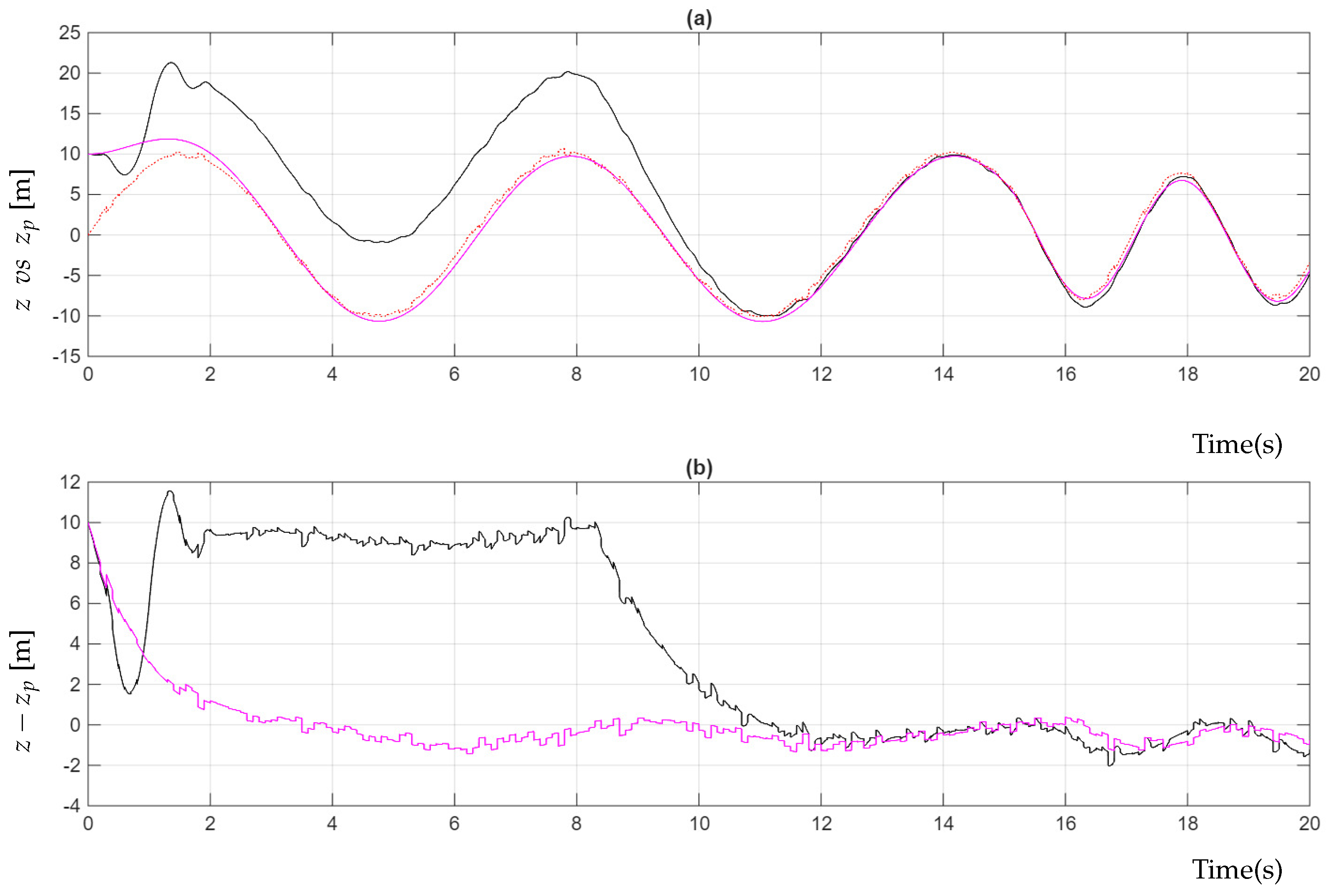
Figure 1 compares the altitude tracking performance of the proposed adaptive internal model regulator (32) and the robust super-twisting sliding-mode controller (52) under low-frequency vertical oscillations of the moving platform. To evaluate the robustness of both controllers against measurement uncertainty, a band-limited white noise signal generated using the MATLAB/Simulink Band-Limited White Noiseblock was added to the platform altitude reference $z_p$. The noise was modeled as a normally distributed process with a noise power of $0.1$ and a sample time of $0.1\mathrm{s}$. The same noise realization was applied to both control strategies to ensure a fair and consistent comparison. As shown in Figure 1a, both controllers successfully synchronize the UAV altitude with the noisy platform trajectory after the initial transient. The adaptive controller exhibits a slower transient response due to the parameter adaptation process, whereas the robust super-twisting sliding-mode controller reaches the reference more rapidly. The corresponding tracking errors, shown in Figure 1b, converge to a small neighborhood around zero, demonstrating satisfactory altitude regulation despite the presence of measurement noise.

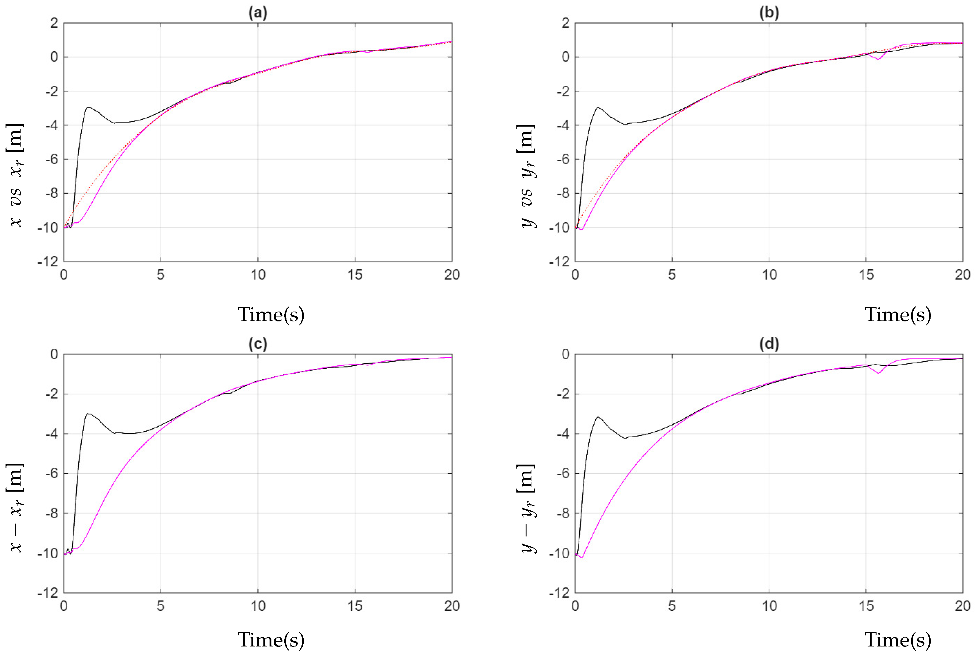
Figure 2 presents the longitudinal and lateral position tracking performance of the proposed adaptive controller (32) and the robust super-twisting sliding-mode controller (52) for the sigmoid reference trajectories under low-frequency platform oscillations. As observed in Figure 2a,b, both control strategies accurately follow the prescribed trajectories after a short transient period, exhibiting nearly indistinguishable steady-state responses. The corresponding tracking errors shown in Figure 2c,d converge close to zero, indicating satisfactory regulation of the horizontal motion. These results demonstrate that both controllers achieve comparable trajectory-tracking performance in the longitudinal and lateral directions under low-frequency operating conditions.

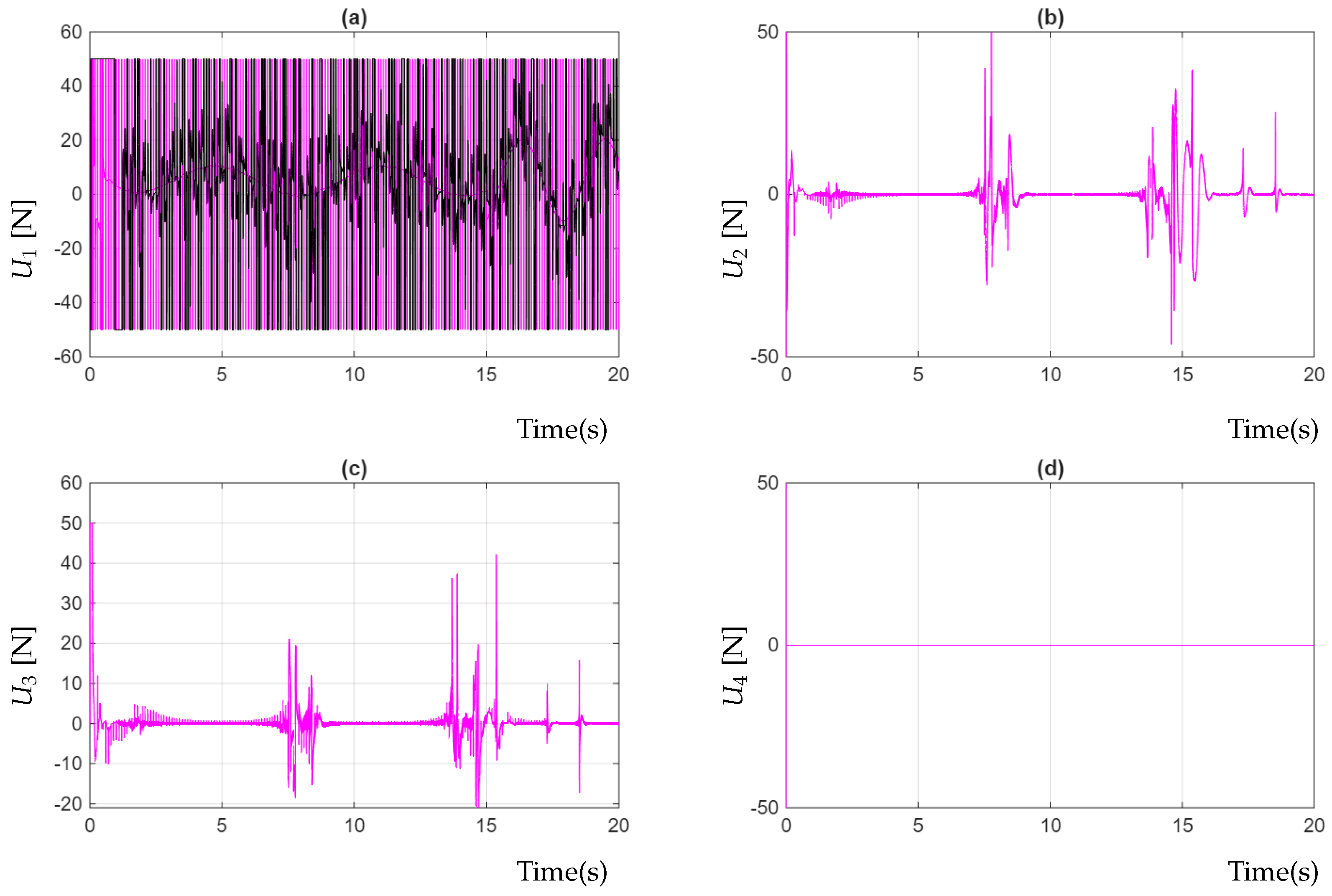
Figure 3 compares the control inputs generated by the proposed adaptive controller (32) and the robust super-twisting sliding-mode controller (52) during the landing maneuver under low-frequency platform oscillations. As shown in Figure 3a, the thrust input $U_1$ exhibits rapid variations associated with altitude regulation and compensation of the platform motion. The control inputs $U_2$ and $U_3$, shown in Figure 3b,c, remain bounded and display nearly identical responses for both control strategies throughout the maneuver. Figure 3d shows that the yaw control input $U_4$ remains close to zero, indicating that no significant yaw actuation is required during the landing process.

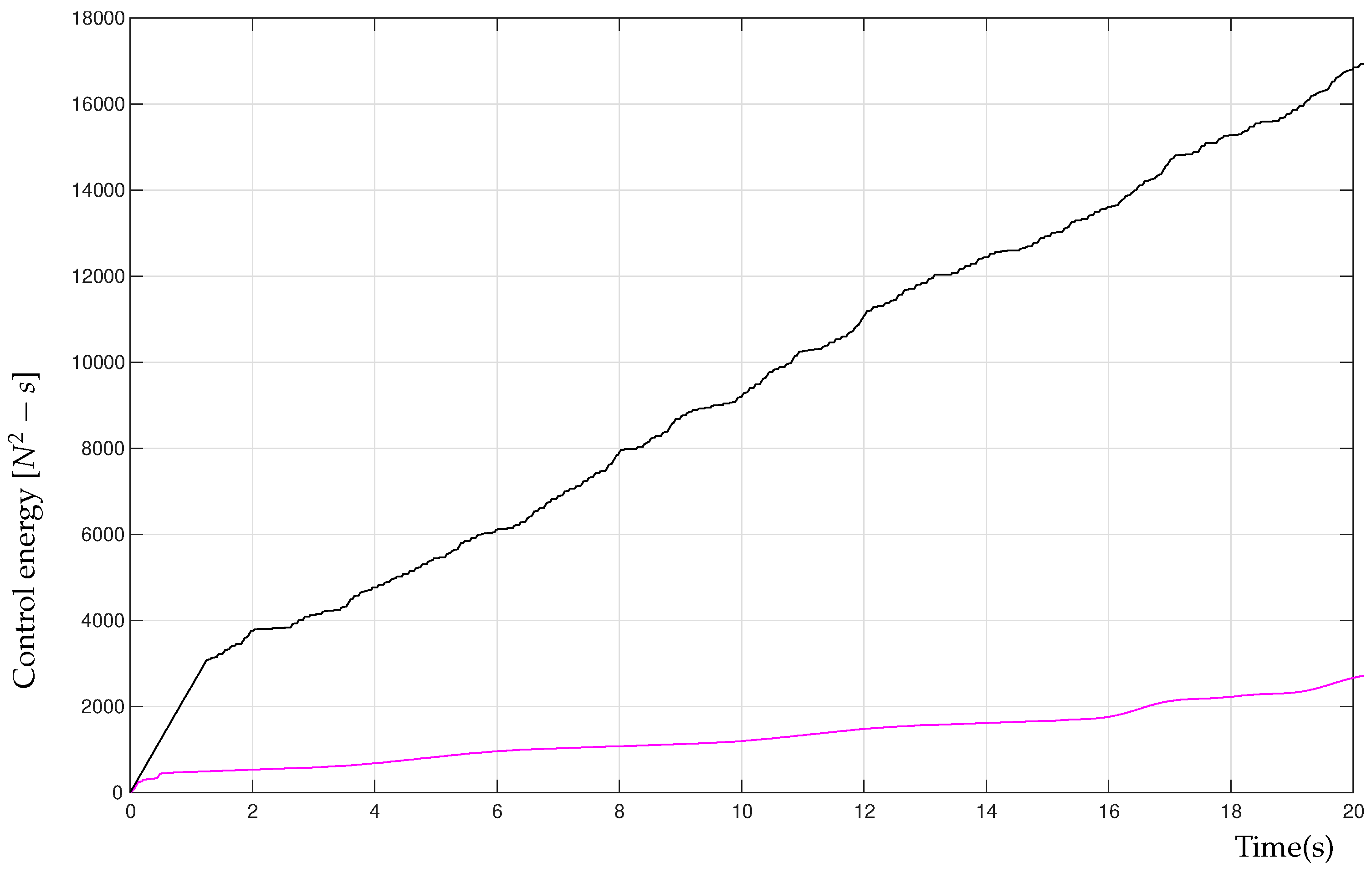
Figure 4 presents the accumulated control energy associated with the thrust input $U_1$ for the proposed adaptive controller (32) and the robust super-twisting sliding-mode controller (52) under low-frequency platform oscillations. The accumulated control energy is computed as the time integral of the squared thrust input, providing a cumulative measure of the control action applied throughout the landing maneuver. As shown in Figure 4, the accumulated control energy increases continuously during the simulation for both control strategies, reflecting the control effort required to compensate for the platform oscillations while maintaining altitude tracking.

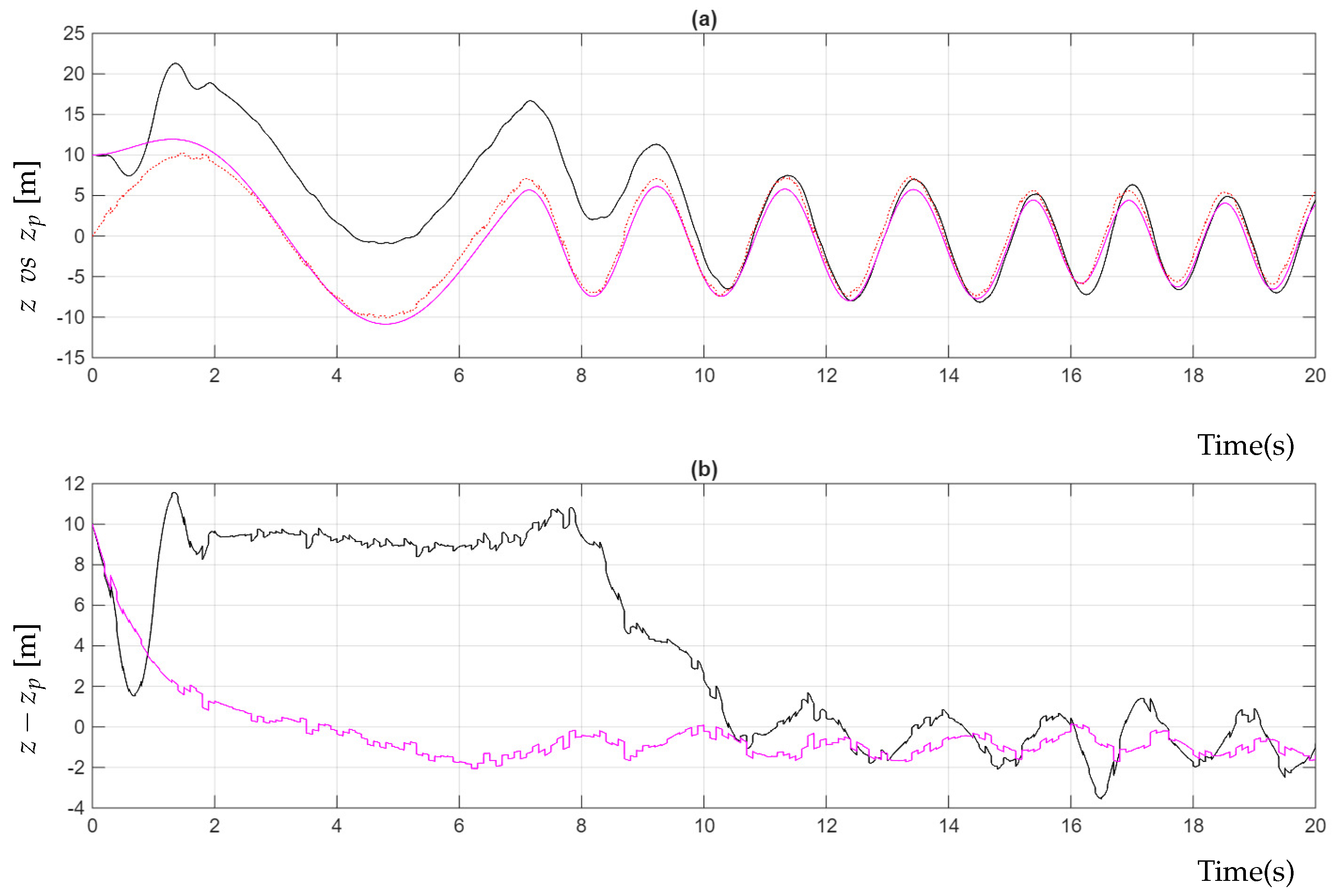
Figure 5 compares the altitude tracking performance of the proposed adaptive internal model regulator (32) and the robust super-twisting sliding-mode controller (52) under high-frequency vertical oscillations of the moving platform. As in the low-frequency case, a band-limited white noise signal generated using the MATLABR2025b/Simulink Band-Limited White Noise block was added to the platform altitude reference $z_p$. The noise was modeled as a normally distributed process with a noise power of $0.1$ and a sample time of $0.1\mathrm{s}$, and the same noise realization was applied to both controllers to ensure identical operating conditions. As shown in Figure 5a, the increase in the platform oscillation frequency makes the altitude tracking problem considerably more demanding. Nevertheless, both controllers remain stable and are able to follow the noisy platform trajectory after the transient response. The corresponding altitude tracking errors, shown in Figure 5b, illustrate the influence of the higher oscillation frequency on the closed-loop response while confirming that the tracking errors remain bounded for both control strategies.

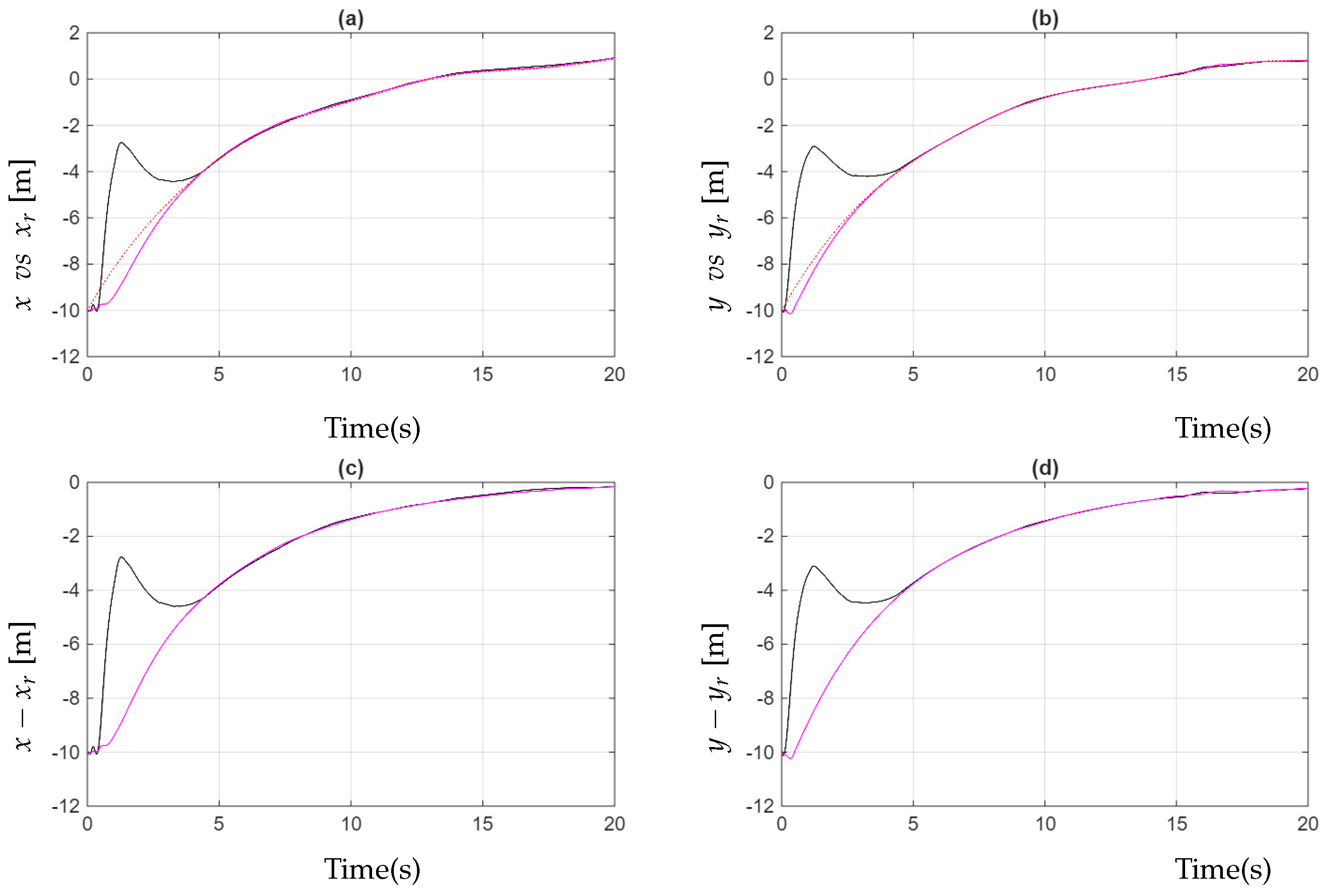
Figure 6 presents the longitudinal and lateral position tracking performance of the proposed adaptive controller (32) and the robust super-twisting sliding-mode controller (52) under high-frequency platform oscillations. As shown in Figure 6a,b, both control strategies follow the prescribed sigmoid reference trajectories after the initial transient, with nearly overlapping responses over most of the simulation interval. The corresponding tracking errors, depicted in Figure 6c,d, decrease progressively and converge to a small neighborhood around zero. These results indicate that the increase in the vertical oscillation frequency does not significantly degrade the longitudinal and lateral tracking performance of either controller.

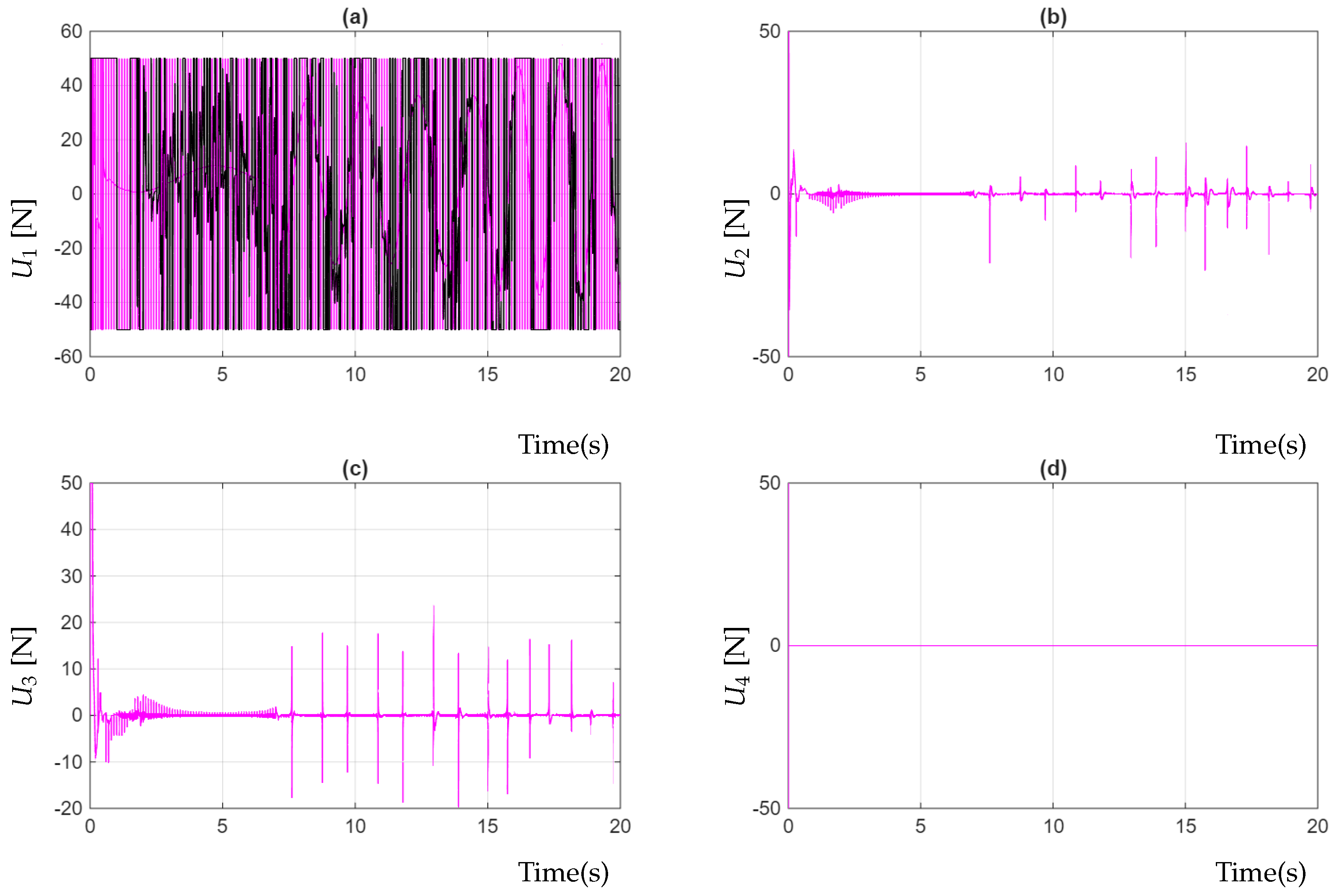
Figure 7 compares the control inputs generated by the proposed adaptive controller (32) and the robust super-twisting sliding-mode controller (52) during the landing maneuver under high-frequency platform oscillations. As shown in Figure 7a, the thrust input $U_1$ exhibits rapid variations, which are required to compensate for the high-frequency vertical motion of the platform while maintaining altitude tracking. The control inputs $U_2$ and $U_3$, depicted in Figure 7b,c, remain bounded throughout the maneuver and display comparable transient responses for both control strategies. Figure 7d shows that the yaw control input $U_4$ remains close to zero during the entire landing process, indicating that no significant yaw actuation is required despite the increase in the platform’s oscillation frequency.

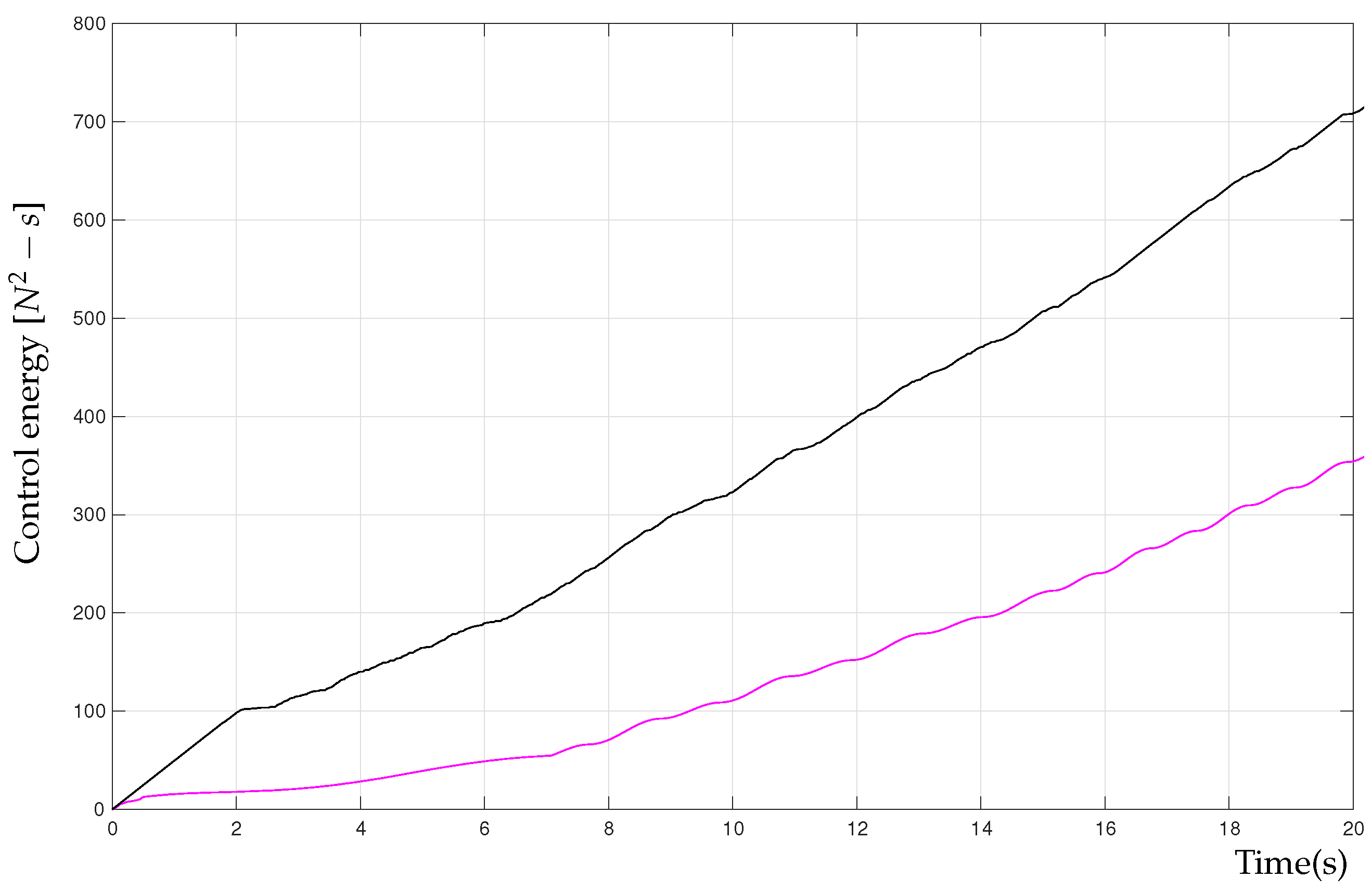
Figure 8 presents the accumulated control energy associated with the thrust input $U_1$ for the proposed adaptive controller (32) and the robust super-twisting sliding-mode controller (52) under high-frequency platform oscillations. The accumulated control energy is computed as the time integral of the squared thrust input, providing a cumulative measure of the control action required throughout the landing maneuver. As shown in Figure 8, the accumulated control energy increases monotonically during the simulation for both control strategies, reflecting the continuous control effort required to compensate for the high-frequency oscillations of the moving platform while maintaining stable altitude tracking.

Table 2. Quantitative tracking performance comparison between the proposed adaptive controller (32) and the robust super-twisting sliding-mode controller (52) under low- and high-frequency platform oscillations. The performance indices correspond to the mean square error (MSE) and accumulated square error (ASE) of the longitudinal, lateral, and altitude tracking errors.

	Low Frequency				High Frequency
	Adaptive Control (32)		Super-Twisting Control (52)		Adaptive Control (32)		Super-Twisting Control (52)
Error	MSE	ASE	MSE	ASE	MSE	ASE	MSE	ASE
$x-x_r$	8.3238	8.3238	14.6391	14.1528	8.5327	8.1573	13.1647	14.6479
$y-y_r$	7.3632	7.1236	14.0310	13.8650	7.4605	6.9605	13.9031	14.0391
$z-z_p$	3.3390	3.1920	4.3876	4.3162	4.2208	4.1028	4.9286	4.4286

summarizes the quantitative tracking performance of the proposed adaptive controller and the robust super-twisting sliding-mode controller for both low- and high-frequency platform oscillations. The comparison is based on the mean square error (MSE) and the accumulated square error (ASE) computed for the longitudinal, lateral, and vertical tracking errors. Under both operating conditions, the proposed adaptive controller achieves lower MSE and ASE values than the robust super-twisting sliding-mode controller for all evaluated tracking variables. The most significant improvement is observed in the altitude tracking error, where the adaptive controller consistently yields substantially smaller error indices, particularly under high-frequency platform oscillations. These quantitative results are consistent with the tracking responses presented in Figure 1, Figure 2, Figure 3, Figure 4, Figure 5 and Figure 6, confirming the effectiveness of the proposed adaptive strategy in maintaining accurate trajectory tracking over a wide range of platform oscillation frequencies.

7. Conclusions

In this work, an autonomous control strategy for a UAV landing on a moving vehicle has been proposed, with particular emphasis on the altitude control subsystem, which plays a critical role in ensuring a safe and reliable landing. The proposed adaptive internal model regulator was compared with a robust super-twisting sliding-mode controller, one of the most widely adopted nonlinear control techniques due to its robustness against uncertainties and external disturbances.

The simulation results show that both controllers successfully accomplish the landing maneuver under low- and high-frequency platform oscillations. The quantitative comparison based on the MSE and ASE performance indices demonstrates that the proposed adaptive internal model regulator consistently achieves lower altitude tracking errors than the robust super-twisting sliding-mode controller in both operating scenarios. These results demonstrate the effectiveness of exploiting the Internal Model Principle to compensate unknown multi-frequency platform oscillations during autonomous UAV landing.

Despite these promising results, several limitations should be acknowledged. The proposed adaptive internal model regulator is particularly well suited for landing platforms whose vertical motion can be represented by periodic or quasi-periodic oscillations. More complex or highly irregular stochastic motions may require more general disturbance models or adaptive estimation techniques. Furthermore, the perception system is assumed to provide accurate measurements of the relative position between the UAV and the landing platform. The effects of sensor noise, vision uncertainties, communication delays, temporary target loss, and sensor failures have not been explicitly addressed and deserve further investigation.

The present study is based on the numerical implementation and simulation-based validation of the proposed adaptive control framework using a nonlinear quadrotor model. Future experimental studies will evaluate the robustness and practical applicability of the proposed methodology under practical or experimental operating conditions, including wind disturbances, actuator saturation, imperfect sensing, communication delays, and terrain-induced platform oscillations.

References

1. Benbassat, D.; Abramson, C. Landing flare accident reports and pilot perception analysis. Int. J. Aviat. Psychol. 2002, 12, 137–152. [Google Scholar] [CrossRef] [PubMed]
2. Chen, X.; Phang, S.K.; Shan, M.; Chen, B.M. System Integration of a Vision-Guided UAV for Autonomous Landing on Moving Platform. In Conference: 2016 12th IEEE International Conference on Control and Automation (ICCA); IEEE: Piscataway, NJ, USA, 2016; pp. 761–766. [Google Scholar]
3. Oualid, A.; Nabil, A.; Ivan, V. Vision Based Autonomous Landing of Multirotor UAV on Moving Platform. J. Intell. Robot. Syst. 2016, 85, 369–384. [Google Scholar] [CrossRef]
4. Rodriguez-Ramos, A.; Sampedro, C.; Bavle, H.; Pascual-Campoy, P. A Deep Reinforcement Learning Strategy for UAV Autonomous Landing on a Moving Platform. J. Intell. Robot. Syst. 2018, 93, 351–366. [Google Scholar] [CrossRef]
5. Battiato, S.; Cantelli, L.; D’urso, F.; Farinella, G.; Guarnera, L.; Guastella, D.; Melita, C.; Muscato, G.; Ortis, A.; Ragusa, F.; et al. A System for Autonomous Landing of a UAV on a Moving Vehicle. In Conference: ICIAP 2017; Springer: Cham, Switzerland, 2017. [Google Scholar]
6. Rodriguez-Ramos, A.; Sampedro, C.; Bavle, H.; Milosevic, Z.; Garcia-Vaquero, A.; Campoy, P. Towards fully autonomous landing on moving platforms for rotary Unmanned Aerial Vehicles. In 2017 International Conference on Unmanned Aircraft Systems (ICUAS); IEEE: Piscataway, NJ, USA, 2017; pp. 170–178. [Google Scholar]
7. Wang, Z.; She, H.; Si, W. Autonomous landing of multi-rotors UAV with monocular gimbaled camera on moving vehicle. In 2017 13th IEEE International Conference on Control & Automation (ICCA); IEEE: Piscataway, NJ, USA, 2017; pp. 408–412. [Google Scholar]
8. Polvara, R.; Sharma, S.; Wan, J.; Manning, A.; Sutton, R. Towards autonomous landing on a moving vessel through fiducial markers. In 2017 European Conference on Mobile Robots (ECMR); IEEE: Piscataway, NJ, USA, 2017; pp. 1–6. [Google Scholar]
9. Hanseob, L.; Seokwoo, J.; David, H.S. Vision-based UAV landing on the moving vehicle. In Conference: 2016 International Conference on Unmanned Aircraft Systems (ICUAS); IEEE: Piscataway, NJ, USA, 2016; pp. 1–7. [Google Scholar]
10. Venugopalan, T.K.; Taher, T.; Barbastathis, G. Autonomous landing of an Unmanned Aerial Vehicle on an autonomous marine vehicle. In 2012 Oceans; IEEE: Piscataway, NJ, USA, 2012; pp. 1–9. [Google Scholar]
11. Nisticò, A.; Baglietto, M.; Simetti, E.; Casalino, G.; Sperindè, A. Marea project: UAV landing procedure on a moving and floating platform. In OCEANS 2017—Anchorage; IEEE: Piscataway, NJ, USA, 2017; pp. 1–10. [Google Scholar]
12. Panjavarnam, K.; Ismail, Z.H.; Tang, C.H.H.; Sekiguchi, K.; Casas, G.G. Model Predictive Control for Autonomous UAV Landings: A Comprehensive Review of Strategies. J. Eng. 2025, 2025, e70085. [Google Scholar] [CrossRef]
13. Xie, J.; Peng, X.; Wang, H.; Niu, W.; Zheng, X. UAV Autonomous Tracking and Landing Based on Deep Reinforcement Learning Strategy. Sensors 2020, 20, 5630. [Google Scholar] [CrossRef] [PubMed]
14. Levant, A. Universal Single-Input–Single-Output (SISO) Sliding-Mode Controllers with Finite Time Convergence. IEEE Trans. Autom. Control 2001, 49, 1447–1451. [Google Scholar] [CrossRef]
15. Obregón–Pulido, G.; Castillo–Toledo, B.; Loukianov, A. A Structurally Stable Globally Adaptive Internal Model Regulator for MIMO Linear Systems. IEEE Trans. Autom. Control 2011, 56, 160–165. [Google Scholar] [CrossRef]
16. Luque-Vega, L.; Castillo-Toledo, B.; Loukianov, A.G. Robust block second order sliding mode control for a quadrotor. J. Frankl. Inst. 2012, 349, 719–739. [Google Scholar] [CrossRef]
17. Francis, B.A. The Linear Multivariable Regulator Problem. SIAM J. Control Optim. 1977, 15, 486–505. [Google Scholar] [CrossRef]
18. Knobloch, H.W.; Isidori, A.; Flockerzi, D. Topics in Control Theory; Birkhäuser Verlag: Berlin, Germany, 1993. [Google Scholar]
19. Davison, E.J. The Robust Control of a Servomechanism Problem for Linear Time–Invariant Multivariable Systems. IEEE Trans. Autom. Control 1976, 21, 25–34. [Google Scholar] [CrossRef]
20. Francis, B.A.; Wonham, W.M. The Internal Model Principle of Control Theory. Automatica 1976, 12, 457–465. [Google Scholar] [CrossRef]
21. Moreno, J.A.; Osorio, M. A Lyapunov approach to second-order sliding mode controllers and observers. In Proceedings of 47th IEEE Conference on Decision and Control (CDC 2008); IEEE: Piscataway, NJ, USA, 2008. [Google Scholar]
22. Zhang, D.; Moreno, J.A.; Reger, J. Parameter preference for the continuous super-twisting-like algorithm based on Hinfty norm analysis. IFAC-PapersOnLine 2020, 53, 5141–5146. [Google Scholar] [CrossRef]
23. Loukianov, A.G. Robust block decomposition sliding mode control design. Int. J. Math. Probl. Eng. Theory Methods Appl. 2002, 8, 349–365. [Google Scholar] [CrossRef]
Figure 1. Altitude tracking under low-frequency oscillations of the moving platform. Comparison between the proposed adaptive controller (32) (black, solid) and the robust super-twisting sliding-mode controller (52) (magenta, solid). (a) UAV altitude response z (19) and platform altitude reference z p (53) (red, dotted). (b) Altitude tracking errors, e z = z z p , corresponding to both control strategies.
Drones 10 00609 g001
Figure 2. Position tracking performance obtained under low-frequency platform oscillations using sigmoid reference trajectories. Comparison between the proposed adaptive controller (32) (black, solid) and the robust super-twisting sliding-mode controller (52) (magenta, solid): (a) longitudinal position x (16) and reference trajectory x r (56) (red, dotted); (b) lateral position y (17) and reference trajectory y r (57) (red, dotted); (c) longitudinal tracking error e x = x x r ; and (d) lateral tracking error e y = y y r .
Drones 10 00609 g002
Figure 3. Control inputs under high-frequency platform oscillations. Comparison between the proposed adaptive controller (32) (black, solid) and the robust super-twisting sliding-mode controller (52) (magenta, solid). (a) U 1 . (b) U 2 . (c) U 3 . (d) U 4 .
Drones 10 00609 g003
Figure 4. Comparison of the accumulated control energy associated with the thrust input U 1 under high-frequency platform oscillations. The proposed adaptive controller (32) (black) and the robust super-twisting sliding-mode controller (52) (magenta).
Drones 10 00609 g004
Figure 5. Comparison of the altitude tracking performance under high-frequency platform oscillations using the proposed adaptive controller (32) (black, solid) and the robust super-twisting sliding-mode controller (52) (magenta, solid): (a) UAV altitude z (19) and platform altitude reference z p (53) (red, dotted); (b) altitude tracking error e z = z z p for both controllers.
Drones 10 00609 g005
Figure 6. Position tracking performance obtained under high-frequency platform oscillations using sigmoid reference trajectories. Comparison between the proposed adaptive controller (32) (black, solid) and the robust super-twisting sliding-mode controller (52) (magenta, solid): (a) longitudinal position x (16) and reference trajectory x r (56) (red, dotted); (b) lateral position y (17) and reference trajectory y r (57) (red, dotted); (c) longitudinal tracking error e x = x x r ; and (d) lateral tracking error e y = y y r .
Drones 10 00609 g006
Figure 7. Control inputs generated by the adaptive control strategy (black) and robust super-twisting sliding-mode controller (magenta) (high-frequency): (a) U 1 ; (b) U 2 ; (c) U 3 ; and (d) U 4 .
Drones 10 00609 g007
Figure 8. Comparison of the accumulated control energy associated with the thrust input U 1 under high-frequency platform oscillations. The proposed adaptive controller (32) (black) and the robust super-twisting sliding-mode controller (52) (magenta).
Drones 10 00609 g008