Robust Trajectory Inference for Quadrotor UAVs Under External Disturbances via a Sliding-Mode-Enhanced CLOE Approach

Highlights

What are the main findings?

• Formal stability guarantees of the trajectory inference scheme are established via a Lyapunov-based analysis, and parameter convergence to constant values is ensured under a persistent excitation condition.
• A robust trajectory inference strategy combining state estimation and parametric identification is proposed within a unified Closed-Loop Output Error (CLOE) framework, incorporating sliding-mode correction terms to ensure convergence under bounded disturbances.

What are the implications of the main findings?

• The theoretical guarantees provided by the Lyapunov-based stability analysis and the persistent excitation condition ensure reliable parameter identifiability and estimation accuracy, as confirmed by simulations carried out in the CoppeliaSim robotics environment.
• The proposed CLOE-based framework provides a complete and physically consistent formulation for trajectory inference of quadrotor systems subject to non-modeled dynamics and external disturbances in three-dimensional space, demonstrating its potential as a robust estimation tool for autonomous aerial systems.

Abstract

This article examines the challenge of trajectory inference for an unknown system affected by external disturbances, with the objective of reconstructing the trajectory of a quadrotor using a reference model. The proposed methodology extends the Closed-Loop Output Error (CLOE) scheme through two complementary contributions: an identified gain, incorporated into the reference model to guarantee the Hurwitz condition of the closed-loop error dynamics, and a set of sliding-mode correction terms that further accelerate error convergence and enhance robustness against bounded disturbances. The stability of both contributions is formally established via Lyapunov-based analysis. The proposed approach is validated through realistic simulations carried out in the CoppeliaSim robotics environment, considering both constant and time-varying trajectory scenarios. Results show that the hybrid approach improves trajectory inference accuracy and convergence speed, maintaining resilience under adverse conditions, making it a promising alternative for autonomous quadrotor monitoring.

1. Introduction

The use of unmanned aerial vehicles (UAVs) has been extended to a wide range of applications, from monitoring remote areas to delivering packages, driven by the advantages of autonomous flight, low cost, and remote operability [1,2,3]. However, controlling these vehicles remains challenging due to the complexity of their dynamics and the presence of external disturbances during flight. To address tasks that exceed the capabilities of a single agent, multi-agent systems (MASs) have emerged as a compelling solution, where multiple quadrotors collaborate to accomplish a specific mission. Depending on the topology of the MAS, each agent must be equipped with control strategies that enable collision avoidance or formation control [4,5,6]. In either case, the ability to infer the trajectories of neighboring agents operating within the same workspace constitutes a fundamental requirement.

In an analogous context, trajectory inference is important for predicting where an autonomous system might be in order to quantify risks, or to reconstruct its position between snapshots of data so as to understand its mission profile or intention. Unlike pure prediction methods, trajectory inference simultaneously addresses the reconstruction of past trajectories, the estimation of unmeasured states, and the anticipation of future motion—making it a fundamental tool for the monitoring and control of autonomous systems in complex operational environments [7,8]. Formally, this problem consists of deducing the trajectory followed by a system from partial and potentially noisy state measurements, combined with prior knowledge of its underlying dynamic model. The trajectory inference problem can be naturally viewed as a combination of state estimation and parametric identification [9], where the goal is not only to reconstruct the internal states of neighboring agents but also to identify the parameters governing their motion.

In the context of quadrotor systems, full-state measurements cannot always be guaranteed due to sensor limitations, hardware faults, or noise corruption, which compromises the reliability of control schemes [10,11]. Since deploying a dedicated sensor for each signal of interest is often infeasible due to cost constraints, technological limitations, or the complexity of the system, estimators emerge as an indispensable tool for reconstructing unmeasured states, identifying unknown parameters, and rejecting external disturbances from available output measurements [12,13]. These estimation objectives are jointly required to keep a system under control, making the estimator design problem a central component of a general control [14,15].

State estimation methodologies can be broadly categorized into two main branches: model-based approaches, such as the Kalman filter, the Luenberger estimators, high-gain estimators, sliding-mode estimators, and adaptive estimators, and data-driven approaches, such as neural network estimators and reinforcement learning-based estimation schemes [16,17,18]. While data-driven methods offer flexibility in the absence of explicit system models, model-based approaches generally require exact or partial knowledge of the mathematical model of the system, which in many practical scenarios is difficult to obtain due to parametric uncertainty, unmodeled dynamics, or the inherent complexity of the system [14,19,20,21].

For example, the Luenberger estimator is formulated under the assumption of a known linear time-invariant model, which considerably limits its applicability to systems where the dynamics are well characterized [22,23]. To address this limitation, high-gain estimators relax the requirement of exact parameter knowledge by employing sufficiently large gains to dominate bounded parametric uncertainty; nevertheless, the system structure must still be known, and excessively high gains can amplify measurement noise, leading to the well-known peaking phenomenon [24,25].

Efforts have been made to address these limitations through methodologies that require only partial knowledge of the system model. In the case of sliding-mode estimators, it is sufficient to know the structure of the model and an upper bound on the uncertainty or disturbance acting on the system, without requiring exact knowledge of the system parameters [26,27,28]. This property makes sliding-mode-based approaches particularly attractive for uncertain systems, since the discontinuous correction term actively rejects bounded disturbances and parametric uncertainty, guaranteeing robust state estimation even in the presence of modeling errors.

Numerous classical approaches for the identification of quadrotor parameters have been proposed, where the authors of [29,30,31,32,33] have addressed this problem through well-established methods, including Levenberg–Marquardt optimization, frequency-domain system identification, subspace model identification, unscented Kalman filtering, low-pass filter-based methods, and practical identification techniques. Despite their individual merits, these techniques share a fundamental constraint: they require, to some extent, explicit knowledge of the mathematical model of the system—whether regarding its architecture, its parameters, or both—thereby considerably limiting their applicability in scenarios where obtaining an accurate model is challenging.

A variety of methodologies have been proposed to jointly address the challenges of state estimation and parameter identification in nonlinear systems, bridging the two problems discussed above. In this regard, refs. [34,35,36,37] have tackled this combined problem through robust controller design under parametric uncertainty, adaptive model predictive control combined with adaptive state estimators, and improved square-root unscented Kalman filtering for online non-stationary parameter estimation. In a similar vein, the ${\mathcal{L}}_1$ adaptive control architecture has been successfully applied to UAV systems, addressing speed regulation, landing control, and hybrid sliding-mode formulations to enhance robustness and adaptation under uncertainties and external disturbances [38,39,40].

The CLOE framework has been extensively employed for parameter identification in mechanical systems, with the authors of references [41,42,43,44] addressing this problem in the context of robot manipulators and general dynamical systems, establishing the theoretical foundations and convergence conditions of this methodology. In the specific context of quadrotor UAVs and trajectory inference, ref. [9] proposed a robust CLOE methodology capable of deducing system dynamics under noisy conditions, later extended in [7] to accommodate partial state measurements by integrating state estimation and parametric identification into a unified framework; nonetheless, both contributions assume linear system dynamics, motivating the present work to extend this approach to the nonlinear dynamics of quadrotor systems undergoing full three-dimensional motion, encompassing translational and rotational movements.

An alternative framework for state estimation encompasses methodologies that do not rely on a precise mathematical characterization of the system; instead, they employ input–output data to infer system states. In this regard, machine learning and deep reinforcement learning approaches have garnered considerable attention for trajectory forecasting and route planning in autonomous systems, with notable applications in autonomous vehicles [17], unmanned aerial vehicles [45,46,47], and mobile robotics [48], showcasing enhancements in adaptability and real-time decision-making under dynamic environments. Along these lines, neural network-based estimator designs, including multi-layer neural network Luenberger estimators with modified back-propagation and dynamic neural network-based sliding-mode estimators, have been proposed for quadrotor state estimation under parameter variations, external disturbances, and sensor noise [49,50]. Nevertheless, these data-driven methodologies typically require extensive training data and considerable computational resources, and fail to deliver formal guarantees regarding estimation error bounds, thereby constraining their applicability in safety-critical contexts [51].

Motivated by the aforementioned limitations and building upon the existing literature, the main contributions of this work can be summarized as follows:

• The linearized quadrotor model explicitly incorporates bounded disturbances and uncertainties—including non-modeled dynamics and wind gusts—while considering fully three-dimensional trajectory tracking, thereby providing a more realistic and complete framework for the trajectory inference problem.
• A robust trajectory inference strategy is proposed, combining state estimation and parametric identification within a unified CLOE approach, ensuring convergence in the presence of external disturbances.
• A Lyapunov-based stability analysis is provided, formally establishing the asymptotic convergence of the estimation error to zero under nominal conditions, and its uniform ultimate boundedness in the presence of bounded disturbances.
• Parameter convergence to constant values is guaranteed under a persistent excitation condition, ensuring the identifiability of the unknown system dynamics.

The outline of the rest of this work is as follows: Section 2 describes the system model and formulates the problem. Section 3 presents the design of the PD control strategy employed to track the reference trajectory. Section 4 presents the trajectory inference scheme and analysis in the sense of Lyapunov. Section 5 presents a robust sliding-mode-based methodology for the trajectory inference algorithm. Section 6 presents the simulation results and their discussion. Finally, Section 7 draws the concluding remarks and outlines directions for future work.

2. System Model and Problem Formulation

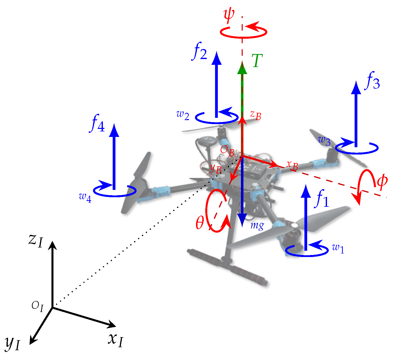
The quadrotor as a rigid body is characterized by a frame linked to it ($B=X_B,Y_B,Z_B$), and with the origin at its center of rotation. The inertial frame $I=X_I,Y_I,Z_I$ is considered fixed with respect to the earth (see Figure 1).

The vector $\xi ={\left[xyz\right]}^{\mathrm{T}}\in {\mathbb{R}}^3$ represents the position of the body-fixed frame origin of the quadcopter expressed at the origin of the inertial frame I. The vehicle orientation is given by a rotation matrix ${}^{I}R_B$, where ${}^{I}R_B\in SO\left(3\right)$ is an orthonormal rotation matrix [52]. In this paper, the $XYZ$ Euler angles, $\eta ={\left[\psi \theta \varphi \right]}^{\mathrm{T}}\in {\mathbb{R}}^3$, have been used to describe the quadcopter rotation matrix ${}^{I}R_B$ with respect to the ground. These angles are bounded as follows: the roll angle $\varphi$ by $(-\pi /2<\varphi <\pi /2)$, the pitch angle $\theta$ by $(-\pi /2<\theta <\pi /2)$, and the yaw angle $\psi$ by $(-\pi <\psi <\pi )$.

The movement of the unmanned aerial vehicle (UAV) results from changes in the lift force caused by adjusting the velocities of the rotors. Longitudinal motions are achieved by means of front and rear rotor velocities, while lateral displacements are performed through the speed of the right and left propellers. Yaw movements are obtained from the difference in the counter-torque between each pair of propellers.

It can be observed in Figure 1 that the four propellers are mounted parallel to the body-fixed $Z_B$ axis, and their rotation axes are orthogonal to the plane defined by $X_B$ and $Y_B$. This configuration allows the vehicle to be controlled by adjusting the thrust of each rotor, providing the total lift along $Z_B$ and producing the necessary rotational moments to achieve the desired orientation and position of the quadrotor.

From Figure 1, it follows that

$$\hat{F}=\left[\begin{array}{c}0\\ 0\\ u\end{array}\right]$$

(1)

where u is the main thrust directed out of the bottom of the aircraft and expressed as

$$u={\displaystyle \sum _{i=1}^4}{f}_i$$

(2)

and, for $i=1,\dots ,4$, $f_i$ is the force produced by motor $M_i$, as shown in Figure 1. Typically $f_i=k_i{\omega }_i^2$, where $k_i$ is a constant and ${\omega }_i$ is the angular speed of the i-th motor. The generalized torques are thus

$$\tilde{\tau }=\left[\begin{array}{c}{\tilde{\tau }}_{\psi }\\ {\tilde{\tau }}_{\theta }\\ {\tilde{\tau }}_{\varphi }\end{array}\right]=\left[\begin{array}{c}{\displaystyle {\sum }_{i=1}^4}{\tilde{\tau }}_{M_i}\\ (f_2-f_4)l\\ (f_3-f_1)l\end{array}\right]$$

(3)

where l is the distance between the motors and the center of gravity, and ${\tau }_{M_i}$ is the moment produced by motor $M_i$, for $i=1,\dots ,4$, around the center of gravity of the aircraft. The reaction torque ${\tau }_{M_i}$ exerted on the airframe about the spin axis of motor $M_i$ arises from the aerodynamic drag on the propeller blades and is typically modeled as ${\tau }_{M_i}=b_i{\omega }_i^2$, where $b_i$ is the drag coefficient of rotor i. Since rotor pairs spin in opposite directions to balance torque in hover, an imbalance in ${\omega }_i$ across rotors produces the net yaw torque ${\tilde{\tau }}_{\psi }={\sum }_{i=1}^4{\tilde{\tau }}_{M_i}$ in (3).

In addition, some assumptions are made to compute the model for control purposes. The ground effect is neglected and the quadcopter airframe is assumed to be symmetric, which results in a moment of inertia tensor of the center of the body-fixed frame with only diagonal inertia terms. Moreover, for control purposes, the center of mass and the body-fixed frame origin are assumed to coincide, which is a common assumption to simplify the dynamic modeling of UAVs.

Under these assumptions, the quadcopter motion equations can be obtained by the Euler–Lagrange formalism based on the kinetic and potential energy concepts. The quadcopter dynamics (see Figure 1) are described by Euler–Lagrange motion equations [3,53,54]:

$$\begin{array}{cc}\hfill m\ddot{x}& =u(sin(\varphi )sin(\psi )+cos(\varphi )cos(\psi )sin(\theta \left)\right)\hfill \end{array}$$

(4)

$$\begin{array}{cc}\hfill m\ddot{y}& =u(cos(\varphi )sin(\theta )sin(\psi )-cos(\psi )sin(\varphi \left)\right)\hfill \end{array}$$

(5)

$$\begin{array}{cc}\hfill m\ddot{z}& =ucos\left(\theta \right)cos\left(\varphi \right)-mg\hfill \end{array}$$

(6)

$$\begin{array}{cc}\hfill \ddot{\psi }& ={\tilde{\tau }}_{\psi }+a\dot{\theta }\dot{\varphi }\hfill \end{array}$$

(7)

$$\begin{array}{cc}\hfill \ddot{\theta }& ={\tilde{\tau }}_{\theta }+b\dot{\psi }\dot{\varphi }\hfill \end{array}$$

(8)

$$\begin{array}{cc}\hfill \ddot{\varphi }& ={\tilde{\tau }}_{\varphi }+c\dot{\theta }\dot{\psi }\hfill \end{array}$$

(9)

where $(x,y,z)\in {\mathbb{R}}^3$ is the position of the mass centre of the quadrotor, while $(\psi ,\theta ,\varphi )\in {\mathbb{R}}^3$ are the yaw angle, the pitch angle, and the roll angle, respectively. The variables $u,{\tilde{\tau }}_{\psi },{\tilde{\tau }}_{\theta },{\tilde{\tau }}_{\varphi }\in \mathbb{R}$ are the control inputs, i.e., the main thrust and the angular moments of the yaw, pitch, and roll angles, respectively.

The term g denotes the acceleration of gravity, and $m\in {\mathbb{R}}_{>0}$ is the mass of the quadrotor. The terms $a={\displaystyle \frac{J_x-J_y}{J_z}},b={\displaystyle \frac{J_y-J_z}{J_x}},c={\displaystyle \frac{J_z-J_x}{J_y}},$ where $J_x$, $J_y$, and $J_z$ are the moments of inertia along the x, y, and z axes, respectively, which are considered unknown.

Equations (4)–(9) are obtained under the following implicit modeling assumptions: (i) the quadrotor is treated as a rigid body; (ii) rotor gyroscopic effects and blade flapping are neglected; (iii) translational aerodynamic drag on the airframe is neglected; and (iv) the body-frame angular rates $(p,q,r)$ are approximated by the time derivatives of the Euler angles, $(p,q,r)\approx (\dot{\varphi },\dot{\theta },\dot{\psi })$, valid for small roll and pitch angles. Consequently, Equations (7)–(9) retain second-order coupling terms and are accurate only up to second order in the Euler angles and their rates.

The moments of inertia $J_x,J_y,J_z$ are assumed to be unknown but constant, strictly positive, and bounded. Since the airframe is assumed symmetric, the inertia tensor is diagonal, with no cross-inertia terms, so that $a,b,$ and c are constant and bounded; the specific quadratic form of Equations (7)–(9) follows from assumption (iv).

Assumption 1.

System (4)–(9) is controllable and only noisy measurements of the generalized coordinates and their derivatives are available, that is, we have access to full state measurements.

Assumption 2.

The control input has an unknown linear structure that does not compromise the closed-loop linearity of (4)–(9).

Problem Formulation

Consider the disturbed quadrotor UAV model with a simplified controlled representation, as shown in (4)–(9). It is desired to infer the generalized coordinates trajectory according to a reference signal ${\zeta }_d\left(t\right)$ via a suitable robust inference trajectory inference scheme despite non-modeled dynamics, external disturbances, and parametric uncertainty acting on the unknown system, respectively.

3. Control

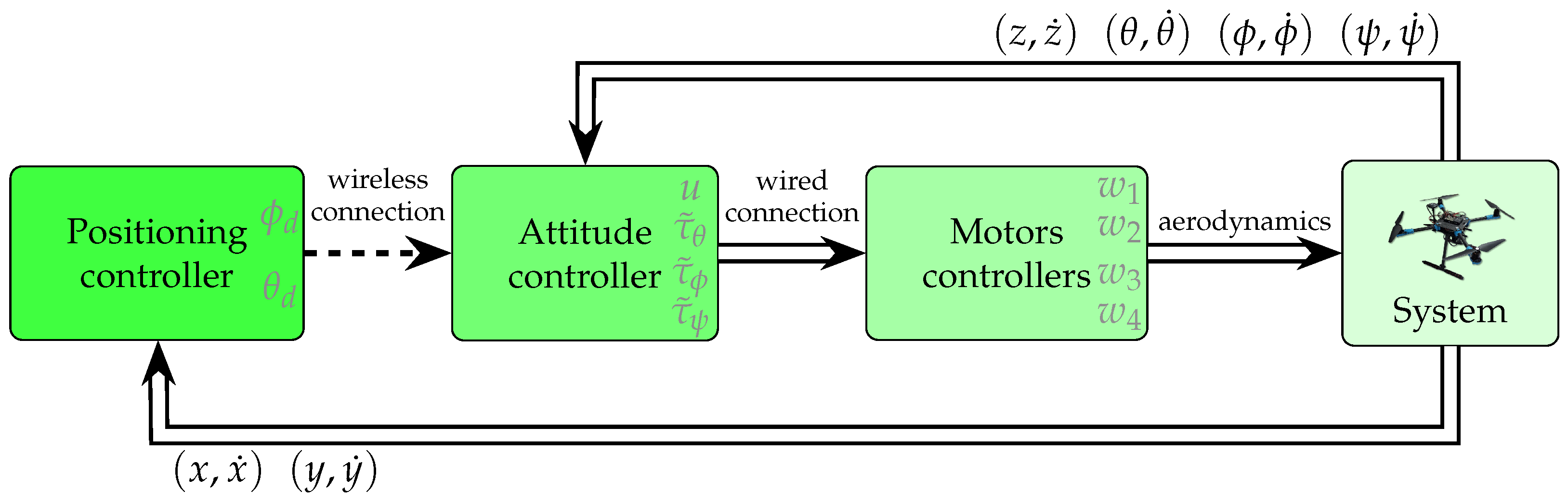
The trajectory control of a quadrotor is implemented following a hierarchical cascaded strategy. Since the position dynamics are decoupled from the attitude dynamics, the overall model can be treated as a series of nested subsystems. In this framework, the altitude and yaw angle are regulated first, followed by the lateral and longitudinal positions together with the pitch and roll angles. The horizontal position controller is considered a high-level module, whereas the attitude controller operates as a low-level component [53]. A general overview of this structure is illustrated in Figure 2, where the darker the shade of green, the higher the control level. In many physical implementations, the position control layer is typically deployed on a ground station and transmitted wirelessly to the vehicle, generating the reference angles required to describe the desired motion along the x and y axes.

The vertical position can be controlled by using the following control input:

$$\begin{array}{cc}\hfill u& =(r_1+mg){\displaystyle \frac{1}{cos\left(\theta \right)cos\left(\varphi \right)}},\hfill \end{array}$$

(10)

where

$$\begin{array}{cc}\hfill r_1& =-k_{v_z}\dot{z}-k_{p_z}{e}_z,\hfill \end{array}$$

(11)

with $e_z=z-z_d$ representing the position error along the z axis, and $z_d$ the desired altitude. The terms $k_{p_z}$ and $k_{v_z}$ are positive control gains. Thus, for altitude control, $r_1$ constitutes a PD controller.

For the yaw angle regulation, a PD control law of the form

$$\begin{array}{cc}\hfill {\tilde{\tau }}_{\psi }& =-k_{v_{\psi }}\dot{\psi }-k_{p_{\psi }}{e}_{\psi }\hfill \end{array}$$

(12)

is considered, where $e_{\psi }=\psi -{\psi }_d$ represents the yaw tracking error, and ${\psi }_d$ is the desired yaw angle. As in the previous case, the gains $k_{v_{\psi }}$ and $k_{p_{\psi }}$ are positive.

Pitch angle is regulated through a PD controller of the form

$$\begin{array}{cc}\hfill {\tilde{\tau }}_{\theta }& =-k_{v_{\theta }}\dot{\theta }-k_{p_{\theta }}(\theta -{\theta }_{\mathrm{ref}}),\hfill \end{array}$$

(13)

where the reference pitch angle is defined as

$$\begin{array}{cc}\hfill {\theta }_{\mathrm{ref}}& =-k_v^x\dot{x}-k_p^x(x-x_d).\hfill \end{array}$$

(14)

Similarly, the roll angle is regulated using a PD controller of the form

$$\begin{array}{cc}\hfill {\tilde{\tau }}_{\varphi }& =-k_{v_{\varphi }}\dot{\varphi }-k_{p_{\varphi }}(\varphi -{\varphi }_{\mathrm{ref}}),\hfill \end{array}$$

(15)

where the roll reference angle is defined as

$$\begin{array}{cc}\hfill {\varphi }_{\mathrm{ref}}& =-k_v^y\dot{y}-k_p^y(y-y_d).\hfill \end{array}$$

(16)

The control parameters $k_{p\psi }$, $k_{v\psi }$, $k_{pz}$, and $k_{vz}$ should be carefully chosen to ensure a stable well-damped response in the vertical and yaw axes [53]. From (6) and (7), it follows that $z\to z_d$ and $\psi \to {\psi }_d$. From (10)–(12) and (6)–(7), $r_1\to 0$ and $\psi \to {\psi }_d$. For a time T large enough, $e_z$ and $e_{\psi }$ are arbitrarily small, therefore, (4) and (5) reduce to

$$\begin{array}{cc}\hfill \ddot{x}& =gtan\theta ,\hfill \end{array}$$

(17)

$$\begin{array}{cc}\hfill \ddot{y}& =-g{\displaystyle \frac{tan\varphi }{cos\theta }}.\hfill \end{array}$$

(18)

Then, if we consider a very small upper bound on $\left|\theta \right|$ and $\left|\varphi \right|$ in such a way that the difference $tan\left(\theta \right)-\theta$ and $tan\left(\varphi \right)-\varphi$ is arbitrarily small, following the standard small-angle linearization approach [53], the system (4)–(9) becomes the following linearized system:

$$\begin{array}{cc}\hfill \ddot{x}& =g\theta +d_x\left(t\right)\hfill \end{array}$$

(19)

$$\begin{array}{cc}\hfill \ddot{y}& =-g\varphi +d_y\left(t\right)\hfill \end{array}$$

(20)

$$\begin{array}{cc}\hfill \ddot{z}& =r_1+d_z\left(t\right)\hfill \end{array}$$

(21)

$$\begin{array}{cc}\hfill \ddot{\psi }& ={\tilde{\tau }}_{\psi }+a\dot{\theta }\dot{\varphi }+d_{\psi }\left(t\right)\hfill \end{array}$$

(22)

$$\begin{array}{cc}\hfill \ddot{\theta }& ={\tilde{\tau }}_{\theta }+b\dot{\psi }\dot{\varphi }+d_{\theta }\left(t\right)\hfill \end{array}$$

(23)

$$\begin{array}{cc}\hfill \ddot{\varphi }& ={\tilde{\tau }}_{\varphi }+c\dot{\theta }\dot{\psi }+d_{\varphi }\left(t\right)\hfill \end{array}$$

(24)

In (19)–(24), couple disturbances are considered under Assumption 2 to capture the effect of unmodeled dynamics, without compromising the stability of the desired trajectory.

Assumption 3.

The terms $d_x,d_y,d_z,d_{\psi },d_{\theta },d_{\varphi }:{\mathbb{R}}_{\ge 0}\to \mathbb{R}$ represent the uncertainties and disturbances in the quadrotor’s dynamics, for instance, non-modeled dynamics and/or wind gusts. It is assumed that such disturbances are uniformly bounded and Lipschitz continuous, i.e., $|d_x\left(t\right)|\le D_x,|d_y\left(t\right)|\le D_y,|d_z\left(t\right)|\le D_z,|d_{\psi }\left(t\right)|\le D_{\psi },|d_{\theta }\left(t\right)|\le D_{\theta },|d_{\varphi }\left(t\right)|\le D_{\varphi },|{\dot{d}}_x\left(t\right)|\le {\overline{D}}_x,|{\dot{d}}_y\left(t\right)|\le {\overline{D}}_y,|{\dot{d}}_z\left(t\right)|\le {\overline{D}}_z,|{\dot{d}}_{\psi }\left(t\right)|\le {\overline{D}}_{\psi },|{\dot{d}}_{\theta }\left(t\right)|\le {\overline{D}}_{\theta },\left|{\dot{d}}_{\varphi }\left(t\right)\right|\le {\overline{D}}_{\varphi },$ for all $t\ge 0$, with known positive constants $D_x,D_y,D_z,D_{\psi },D_{\theta },D_{\varphi },{\overline{D}}_x,{\overline{D}}_y,{\overline{D}}_z,{\overline{D}}_{\psi },{\overline{D}}_{\theta },{\overline{D}}_{\varphi }$.

4. Trajectory Inference

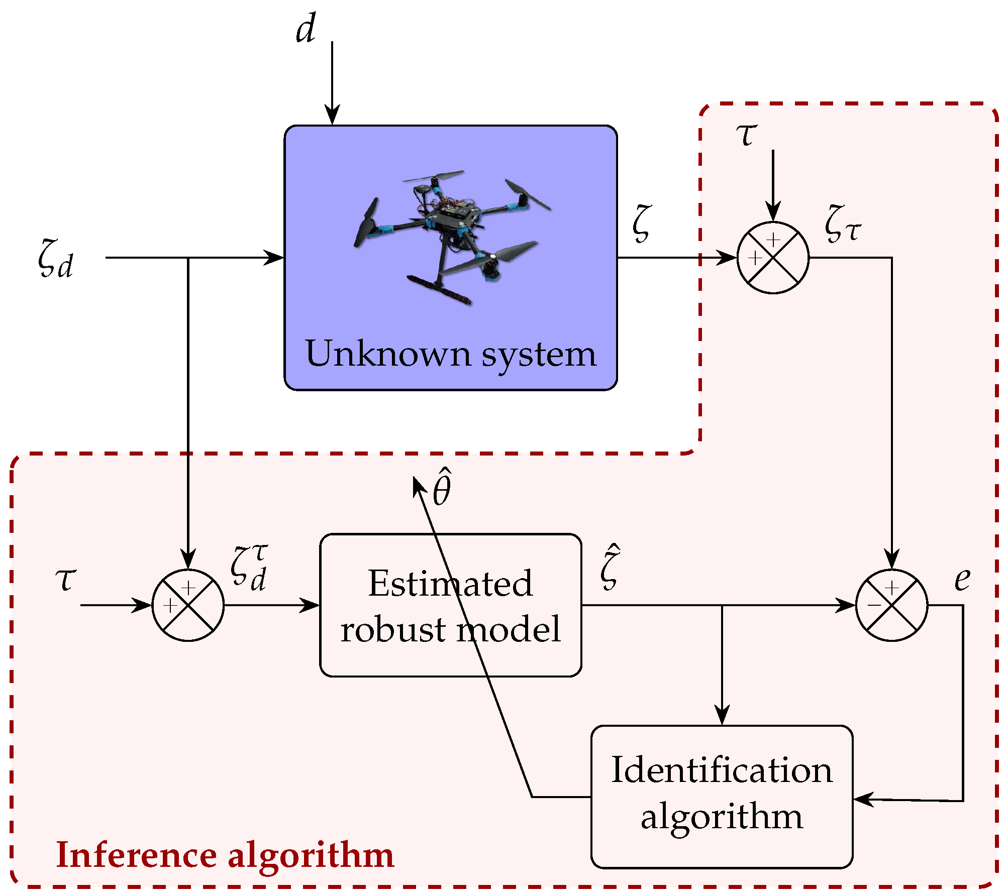
The proposed CLOE algorithm is illustrated in Figure 3. An estimated model of the perturbed unknown system is constructed such that the mismatch between the measured outputs and their robust estimated counterparts drives an identification algorithm, which iteratively refines the model parameters.

This closed-loop structure yields a model matching framework [55], in which the estimated model is driven to replicate the input–output behavior of the unknown system, a concept well established in adaptive control theory [56]. The resulting identified model faithfully captures the underlying system dynamics, constituting a physics-informed representation that encodes the structural knowledge of the quadrotor model within the estimation scheme. This identified model can subsequently serve as a basis for trajectory prediction algorithms, including those based on physics-informed approaches [8].

The proposed inference algorithm combines a state observer with an online parameter identification scheme, jointly exploiting the strengths of both approaches to reconstruct the underlying physics-informed reference model of the unknown system from real-time full-state measurements, without requiring prior knowledge of its dynamics [9].

Given the underlying nature of the system, the full model admits a decomposition into four structurally decoupled subsystems: two fourth-order subsystems associated with the x-$\theta$ and y-$\varphi$ motions, and two second-order subsystems corresponding to the altitude z and yaw $\psi$ channels. Nevertheless, from (19)–(23), (20)–(24), (22) and (21), the complete system can be expressed in a unified state-space representation as

$$\begin{array}{cc}\hfill \dot{\zeta }=& \mathcal{A}\zeta +\mathcal{B}U.\hfill \end{array}$$

(25)

Considering $U={[{\tilde{\tau }}_{\theta },{\tilde{\tau }}_{\varphi },{\tilde{\tau }}_{\psi },r_1]}^{\top }$ and ${\zeta }_d={[x_d,y_d,{\psi }_d,z_d]}^{\top }$, the closed-loop system can be expressed as

$$\begin{array}{cc}\hfill \dot{\zeta }=& {\mathcal{A}}_c\zeta +{\mathcal{B}}_c{\zeta }_d={\Phi }^{\mathrm{T}}\Theta ,\hfill \end{array}$$

(26)

where ${\mathcal{A}}_c,{\mathcal{B}}_c\in {\mathbb{R}}^{12\times 12}$ are the closed-loop matrices resulting from the interconnection of the quadrotor dynamics and the stabilizing control law, and are treated as unknown for the purposes of the proposed trajectory inference scheme. Here, $\Phi \in {\mathbb{R}}^{16\times 12}$ is the regressor matrix and $\Theta \in {\mathbb{R}}^{1}6$ is the parameter vector, defined, respectively, as

$$\Phi =\left[\begin{array}{c}I\otimes \zeta \\ I\otimes {\zeta }_d\end{array}\right],\Theta =\left[\begin{array}{c}\mathrm{vec}\left({\mathcal{A}}_c\right)\\ \mathrm{vec}\left({\mathcal{B}}_c\right)\end{array}\right].$$

Here, ⊗ denotes the Kronecker product, and $\mathrm{vec}(·)$ denotes the vectorization operator, which stacks the columns of a matrix into a single column vector. The closed-loop system (26) does not incorporate an excitation signal $\tau$ in the desired reference ${\zeta }_d$. To satisfy the persistent excitation condition required for parameter convergence, an auxiliary probing signal is injected into the reference input solely for identification purposes. Since this signal is known a priori, it can be subsequently removed from the reference to recover the original desired trajectory ${\zeta }_d$. It is noted that the excitation signal $\tau$, composed of sinusoidal terms at multiple frequencies, is frequency-rich by construction, which breaks the linear dependency between the reference input and the state and constitutes a standard sufficient condition to secure the lower bound ${\beta }_1>0$ in the persistent excitation condition (41), consistent with classical results in adaptive identification [57]. Under this consideration, the augmented reference signal takes the form

$$\begin{array}{cc}\hfill {\dot{\zeta }}_{\tau }=& {\mathcal{A}}_c{\zeta }_{\tau }+{\mathcal{B}}_c({\zeta }_d+\tau )={\Phi }^{\mathrm{T}}\Theta ,\hfill \end{array}$$

(27)

where

$$\begin{array}{cc}\hfill \Phi & =\left[\begin{array}{c}I\otimes {\zeta }_{\tau }\\ I\otimes ({\zeta }_d+\tau )\end{array}\right].\hfill \end{array}$$

The reference model takes the form of

$$\begin{array}{cc}\hfill \dot{\hat{\zeta }}=& {\hat{\mathcal{A}}}_c\hat{\zeta }+{\hat{\mathcal{B}}}_c({\zeta }_d+\tau )+\mathcal{L}({\zeta }_{\tau }-\hat{\zeta })={\Phi }_m^T\hat{\Theta }+\mathcal{L}({\zeta }_{\tau }-\hat{\zeta }),\hfill \end{array}$$

(28)

where ${\hat{\mathcal{A}}}_c,{\hat{\mathcal{B}}}_c$ are built from the parameters identified online for the closed-loop matrices ${\mathcal{A}}_c,{\mathcal{B}}_c$, and

$${\Phi }_m=\left[\begin{array}{c}I\otimes \hat{\zeta }\\ I\otimes ({\zeta }_d+\tau )\end{array}\right],\hat{\Theta }=\left[\begin{array}{c}\mathrm{vec}\left({\hat{\mathcal{A}}}_c\right)\\ \mathrm{vec}\left({\hat{\mathcal{B}}}_c\right)\end{array}\right].$$

$\mathcal{L}=\mathrm{diag}(l_1,\dots ,l_{12})\in {\mathbb{R}}^{12\times 12}$ is an additional parameter, designed to ensure that the closed-loop matrix ${\mathcal{A}}_c-\mathcal{L}$ remains Hurwitz. Specifically, $\mathcal{L}$ is updated component-wise according to

$$\begin{array}{c}\hfill {\dot{l}}_i={\gamma }_i{e}_i^2,i=1,\dots ,12,\end{array}$$

(29)

or, equivalently, in compact matrix form,

$$\begin{array}{c}\hfill \dot{L}={\Gamma }_L\mathrm{diag}\left(e_1^2,\dots ,e_{12}^2\right),{\Gamma }_L=\mathrm{diag}({\gamma }_1,\dots ,{\gamma }_{12})>0.\end{array}$$

(30)

Hence, the output error is defined as

$$\begin{array}{cc}\hfill e& ={\zeta }_{\tau }-\hat{\zeta },\hfill \end{array}$$

(31)

then

$$\begin{array}{cc}\hfill \dot{e}& ={\dot{\zeta }}_{\tau }-\dot{\hat{\zeta }}\hfill \\ & ={\mathcal{A}}_c{\zeta }_{\tau }+{\mathcal{B}}_c({\zeta }_d+\tau )-{\hat{\mathcal{A}}}_c\hat{\zeta }-{\hat{\mathcal{B}}}_c({\zeta }_d+\tau )-\mathcal{L}(\zeta -\hat{\zeta })\hfill \\ \hfill & =({\mathcal{A}}_c-\mathcal{L})e-{\Phi }_m^{\mathrm{T}}\tilde{\Theta },\hfill \end{array}$$

(32)

where $\tilde{\Theta }$ is parametric error defined as

$$\begin{array}{cc}\hfill \tilde{\Theta }=& \hat{\Theta }-\Theta =\left[\begin{array}{c}\mathrm{vec}\left({\hat{\mathcal{A}}}_c-{\mathcal{A}}_c\right)\\ \mathrm{vec}\left({\hat{\mathcal{B}}}_c-{\mathcal{B}}_c\right)\end{array}\right].\hfill \end{array}$$

Theorem 1.

Consider full-state measurements of a linear time-invariant system of (27) and the reference model (28). If the parameters $\hat{\Theta }$ are updated as

$$\begin{array}{c}\hfill \dot{\hat{\Theta }}=\Gamma {\Phi }_{m}e,\end{array}$$

(33)

where $\Gamma \in {\mathbb{R}}^{p\times p}$ is a positive-definite gain matrix, and $\mathcal{L}-{\mathcal{A}}_c>0$, then $\hat{\Theta }$, e, $\hat{\zeta }$ and ${\Phi }_m$ remain bounded and the dynamic error (32) converges to 0.

Proof. 

We proposed a Lyapunov function based on estimation error

$$\begin{array}{cc}\hfill V\left(e\right)=& {\displaystyle \frac{1}{2}}{e}^{\mathrm{T}}e+{\displaystyle \frac{1}{2}}{\tilde{\Theta }}^{\mathrm{T}}{\Gamma }^{-1}\tilde{\Theta }.\hfill \end{array}$$

(34)

It can be observed that the proposed Lyapunov function is positive definite. Taking the time derivative of the Lyapunov function yields

$$\begin{array}{cc}\hfill \dot{V}\left(e\right)=& e^{\mathrm{T}}\dot{e}+{\tilde{\Theta }}^{\mathrm{T}}{\Gamma }^{-1}\dot{\tilde{\Theta }}\hfill \\ \hfill =& e^{\mathrm{T}}\left[({\mathcal{A}}_c-\mathcal{L})e-{\Phi }_m^T\tilde{\Theta }\right]+{\tilde{\Theta }}^{\mathrm{T}}{\Gamma }^{-1}[{\Phi }_m\Gamma e]\hfill \\ \hfill =& e^{\mathrm{T}}({\mathcal{A}}_c-\mathcal{L})e-e^{\mathrm{T}}{\Phi }_m^{\mathrm{T}}\tilde{\Theta }+{\tilde{\Theta }}^{\mathrm{T}}{\Phi }_{m}e\hfill \\ \hfill =& -e^{\mathrm{T}}(\mathcal{L}-{\mathcal{A}}_c)e\le -{\lambda }_{min}(\mathcal{L}-{\mathcal{A}}_c){\parallel e\parallel }^2,\hfill \end{array}$$

(35)

provided that $\mathcal{L}-{\mathcal{A}}_c>0$. From the above inequality, the boundedness of e can be concluded, that is, $e\in {\mathcal{L}}_{\infty }$, and also that $V\left(0\right)\ge V\left(t\right)$ for any time instance t. Furthermore, the boundedness of e implies the boundedness of the estimated states $\hat{\zeta }$; and, hence, the regressor matrix ${\Phi }_m$ is also bounded. So, $e,\hat{\zeta },{\Phi }_m\in {\mathcal{L}}_{\infty }$.

If we integrate both sides of the above inequality in a time interval $[0,t]$, it follows that

$$\begin{array}{cc}\hfill V\left(t\right)-V\left(0\right)& \le -{\lambda }_{min}(\mathcal{L}-{\mathcal{A}}_c){\int }_0^t{\parallel e\parallel }^{2}d\tau ,\hfill \\ \hfill V\left(0\right)& \ge V\left(0\right)-V\left(t\right)\ge {\lambda }_{min}(\mathcal{L}-{\mathcal{A}}_c){\int }_0^t{\parallel e\parallel }^{2}d\tau .\hfill \end{array}$$

(36)

Then, it follows that

$$\begin{array}{c}\hfill {\int }_0^t{\parallel e\parallel }^{2}d\tau \le {\displaystyle \frac{V\left(0\right)}{{\lambda }_{min}(\mathcal{L}-{\mathcal{A}}_c)}}<\infty .\end{array}$$

(37)

From the above expression, it follows that e is an ${\mathcal{L}}_2$ function. Since the parametric error $\tilde{\Theta }$ and the signals within e are bounded, this allows the conclusion that $\dot{e}$ is also bounded, that is, $\dot{e}\in {\mathcal{L}}_{\infty }$. Barbalat’s lemma is applied to conclude that e converges to 0. This completes the proof. □

Remark 1.

Note that $\mathcal{L}$ plays an essential stabilizing role in the closed-loop error dynamics; it can be designed as an adaptive stabilizing gain whose sole purpose is to guarantee the Hurwitz condition of ${\mathcal{A}}_c-\mathcal{L}$.

The matrix $\Phi$ must satisfy the following persistent excitation conditions for the parametric identification that feeds the estimated model.

Definition 1

(Persistent Excitation [12]). The regressor matrix ${\Phi }_i\left(t\right)$ of the i-th subsystem block, $i=1,2,3,4$, is said to be persistently exciting (PE) if there exist constants ${\beta }_{1i},{\beta }_{2i},T_i>0$ such that, for all $t\ge 0$,

$${\beta }_{1i}I\le {\int }_t^{t+T_i}{\Phi }_i^{\top }\left(\tau \right){\Phi }_i\left(\tau \right)d\tau \le {\beta }_{2i}I,$$

(38)

where ${\Phi }_i\in {\mathbb{R}}^{p_i\times n_i}$ depends on the estimated states ${\hat{\zeta }}_i$ and the augmented reference ${\zeta }_{d,i}+{\tau }_i$.

Lemma 1.

The parameter update law

$${\dot{\hat{\Theta }}}_i={\Gamma }_i{\Phi }_i^{\top }\left(t\right)e_i\left(t\right),{\Gamma }_i\in {\mathbb{R}}^{p_i\times p_i},{\Gamma }_i>0,$$

(39)

and the linear time-varying (LTV) system

$${\dot{w}}_i=B_i\left(t\right)u_i,z_i=C_i\left(t\right)w_i,$$

(40)

are equivalent under the identification $u_i\equiv e_i$, $B_i\left(t\right)\equiv {\Gamma }_i{\Phi }_i^{\top }\left(t\right)$, $C_i\left(t\right)\equiv {\Phi }_i\left(t\right)$, and $w_i\equiv {\tilde{\Theta }}_i$, where ${\tilde{\Theta }}_i={\Theta }_i-{\hat{\Theta }}_i$ denotes the parametric error vector of the i-th block. Furthermore, the PE condition (38) is equivalent to the uniform complete observability (UCO) of system (40), i.e., the observability Gramian

$${\mathcal{N}}_i(t,t+T_i)={\int }_t^{t+T_i}{C}_i^{\top }\left(\tau \right)C_i\left(\tau \right)d\tau ={\int }_t^{t+T_i}{\Phi }_i^{\top }\left(\tau \right){\Phi }_i\left(\tau \right)d\tau ,$$

(41)

satisfies (38). Consequently, if $e_i$ and $z_i$ are bounded, then ${\tilde{\Theta }}_i$ is bounded for all $i=1,2,3,4$.

Proof. 

The equivalence between (39) and (40) follows directly from the substitution $u_i=e_i$, $B_i\left(t\right)={\Gamma }_i{\Phi }_i^{\top }\left(t\right)$, $C_i\left(t\right)={\Phi }_i\left(t\right)$, and $w_i={\tilde{\Theta }}_i$, since

$${\dot{\tilde{\Theta }}}_i={\dot{\hat{\Theta }}}_i={\Gamma }_i{\Phi }_i^{\top }\left(t\right)e_i\left(t\right)=B_i\left(t\right)u_i.$$

(42)

The observability Gramian ${\mathcal{N}}_i(t,t+T_i)$ of system (40) coincides with the integral in (38); hence, the PE condition is equivalent to the UCO of (40). Under UCO, if the input $u_i=e_i$ and the output $z_i={\Phi }_i\left(t\right){\tilde{\Theta }}_i$ are bounded, then by the boundedness property of UCO systems [58], $w_i={\tilde{\Theta }}_i$ is bounded. The boundedness of $e_i$ follows from the Lyapunov analysis of the estimator–identifier scheme (Theorem 1), and $z_i$ is bounded since ${\Phi }_i\in L_{\infty }$ and ${\tilde{\Theta }}_i\in L_{\infty }$. This holds for all four blocks $i=1,2,3,4$, completing the proof. □

Remark 2.

The user-defined excitation signal ${\tau }_i\in {\mathcal{C}}^1$, added to the augmented reference ${\chi }_{d,i}+{\tau }_i$, guarantees that the regressor ${\Phi }_i\left(t\right)$ does not lose rank over any window of length $T_i$, even when the reference trajectory ${\chi }_{d,i}\left(t\right)$ is not sufficiently rich. In particular, for subsystems $i=1,2$ (four-integrator chains) the signal ${\tau }_i$ must excite at least $p_i$ distinct frequencies, while for subsystems $i=3,4$ (two-integrator chains) the requirement is relaxed accordingly. A sufficient choice is a linear combination of sinusoidal signals with rationally independent frequencies, which ensures condition (38) for all blocks.

5. Sliding-Mode Approach

Taking into account the dynamic model expressed in (27), the formulation is extended to all blocks, yielding the 12 states defined as $\zeta ={[x,\dot{x},\theta ,\dot{\theta },y,\dot{y},\varphi ,\dot{\varphi },\psi ,\dot{\psi },z,\dot{z}]}^{\top }\in {\mathbb{R}}^{12}$, where $(x,y,z)$ are the position coordinates in the inertial frame and $(\varphi ,\theta ,\psi )$ are the Euler angles describing the vehicle attitude.

The update law operates on the estimation error $e\left(t\right)=\zeta \left(t\right)-\hat{\zeta }\left(t\right)$ and produces an update of the identified parameters $\hat{\Theta }\in {\mathbb{R}}^p$ of the form

$$\begin{array}{cc}\hfill \dot{\hat{\Theta }}& =\Gamma {\Phi }_{m}e,\hfill \end{array}$$

(43)

where $\Gamma \in {\mathbb{R}}^{p\times p}$ is a positive-definite adaptive gain matrix, and ${\Phi }_m$ is the regressor matrix that depends on both the measured states $\zeta$ and the estimated states $\hat{\zeta }$.

In order to improve the robustness of the scheme against parametric uncertainties and unmodeled disturbances of the unknown system, the estimated model is complemented with an estimator based on high-order sliding modes, specifically the exact estimator of Levant.

The Levant-based high-order sliding-mode estimator of order n is given by

$$\begin{array}{cc}\hfill {\dot{\hat{\zeta }}}_1& ={\hat{\zeta }}_2-{\alpha }_1{\overline{\delta }}^{p_1}{\lfloor e_1\rceil }^{p_1},\hfill \\ \hfill {\dot{\hat{\zeta }}}_2& ={\hat{\zeta }}_3-{\alpha }_2{\overline{\delta }}^{p_2}{\lfloor e_1\rceil }^{p_2},\hfill \\ \hfill & ⋮\hfill \\ \hfill {\dot{\hat{\zeta }}}_{n-1}& ={\hat{\zeta }}_n-{\alpha }_{n-1}{\overline{\delta }}^{p_{n-1}}{\lfloor e_1\rceil }^{p_{n-1}},\hfill \\ \hfill {\dot{\hat{\zeta }}}_n& =-{\alpha }_n\overline{\delta }sign\left(e_1\right),\hfill \end{array}$$

(44)

where $e_1={\zeta }_1-{\hat{\zeta }}_1$ is the error in the first state, ${\lfloor e_1\rceil }^{p_i}\triangleq {\left|e_1\right|}^{p_i}\mathrm{sign}\left(e_1\right)$ with exponents $p_i$ decreasing along the estimation chain, $\overline{\delta }>0$ is an upper bound on the disturbance, and ${\alpha }_i>0$ are the estimator gains, whose nominal values have been reported in [59]. A fundamental property of this scheme is that, under appropriate gain conditions, the observation error converges to zero in finite time $t_s>0$, so that $e_i\left(t\right)={\zeta }_i\left(t\right)-{\hat{\zeta }}_i\left(t\right)=0$ for all $t\ge t_s$ and for all $i\in \{1,\dots ,n\}$ [60].

Recall that the unknown system is assumed to be affected by a disturbance; accordingly, a representative disturbance term $\delta \left(t\right)$ is incorporated into the closed-loop dynamics (27). Subtracting the reference model (28), complemented with the sliding-mode correction term, from the resulting disturbed closed-loop system yields the observation error dynamics presented below.

In contrast to the classical Levant estimator, where only $e_1$ is available, the proposed scheme exploits the full-state measurement to assign an independent correction term to each state. Since all state measurements are accessible, the standard high-order sliding-mode observer structure can be directly applied to each state, yielding the following estimator for the complete 12-dimensional system

$$\dot{e}=({\mathcal{A}}_c-\mathcal{L})e-{\Phi }^{\top }\tilde{\theta }+\Lambda {\lfloor e\rceil }^p+\delta \left(t\right),$$

(45)

where $e\in {\mathbb{R}}^{12}$, $\Lambda =\mathrm{diag}({\alpha }_1,\dots ,{\alpha }_{12})>0$, ${\lfloor e\rceil }^p={\left[{\lfloor e_1\rceil }^{p_1},\dots ,{\lfloor e_{12}\rceil }^{p_{12}}\right]}^{\top }$ with ${\lfloor e_i\rceil }^{p_i}\triangleq {\left|e_i\right|}^{p_i}\mathrm{sign}\left(e_i\right)$, $0\le p_i<1$, and $\delta \left(t\right)\in {\mathbb{R}}^{12}$ is a bounded disturbance satisfying $|{\delta }_i\left(t\right)|\le {\overline{\delta }}_i$ for all $i=1,\dots ,12$.

The following statement establishes the stability properties of the resulting error dynamics (45), incorporating both the identified gain $\mathcal{L}$ and the sliding-mode correction terms, under the presence of bounded disturbances.

Theorem 2.

Under the same identification framework and update law established in Theorem 1 for $\hat{\Theta }$, and satisfying $\mathcal{L}-{\mathcal{A}}_c>0$ for all $t\ge 0$, and assuming further that ${\alpha }_i>0$ for all $i=1,\dots ,12$, the trajectories of (45) are uniformly ultimately bounded (UUB), converging to a compact set whose radius is explicitly determined by ${\overline{\delta }}_i$, ${\alpha }_i$, and $p_i$.

Proof. 

Consider the augmented Lyapunov function

$$V={\displaystyle \frac{1}{2}}{e}^{\top }e+{\displaystyle \frac{1}{2}}{\tilde{\theta }}^{\top }{\Gamma }^{-1}\tilde{\theta },$$

(46)

which is positive definite, since it is the sum of two non-negative terms that vanish only at the origin.

Differentiating along the trajectories of (45) and substituting $\dot{\hat{\theta }}=\Gamma \Phi e$, the parametric terms cancel exactly as in Theorem 1:

$$\dot{V}=-e^{\top }(\mathcal{L}-{\mathcal{A}}_c)e+e^{\top }\Lambda {\lfloor e\rceil }^p+e^{\top }\delta \left(t\right).$$

(47)

By the identification framework and update law established in Theorem 1, condition ${\mathcal{A}}_c-\mathcal{L}>0$ holds, so that

$$e^{\top }({\mathcal{A}}_c-\mathcal{L})e\le -{\lambda }_{min}(\mathcal{L}-{\mathcal{A}}_c){\parallel e\parallel }^2.$$

(48)

For each $i=1,\dots ,12$, define

$$f_i\left(\right|e_i\left|\right)\triangleq {\alpha }_i|e_i{|}^{p_i+1}-{\overline{\delta }}_i\left|e_i\right|.$$

(49)

Since $p_i+1\in (1,2)$, the function $f_i$ is not sign-definite for all $|e_i|$: it is negative near the origin (where the linear disturbance term dominates) and positive for sufficiently large $|e_i|$. To obtain a valid bound, the minimum of $f_i$ is computed explicitly. Setting

$${\displaystyle \frac{d}{d|e_i|}}\left[{\overline{\delta }}_i|e_i|-{\alpha }_i{\left|e_i\right|}^{p_i+1}\right]=0⟹{\overline{\delta }}_i={\alpha }_i(p_i+1){\left|e_i\right|}^{p_i},$$

(50)

yields the minimizer

$$|e_i{|}^{\ast }={\left({\displaystyle \frac{{\overline{\delta }}_i}{{\alpha }_i(p_i+1)}}\right)}^{1/p_i}.$$

(51)

Evaluating $f_i$ at $|e_i{|}^{\ast }$ gives the finite, explicitly computable constant

$$m_i\triangleq -f_i(|e_i{|}^{\ast })={\overline{\delta }}_i{\left|e_i\right|}^{\ast }-{\alpha }_i{\left(|e_i{|}^{\ast }\right)}^{p_i+1}\ge 0,$$

(52)

so that

$$f_i\left(\right|e_i\left|\right)\ge -m_i\forall \left|e_i\right|\ge 0.$$

(53)

Summing over all channels,

$$e^{\top }\Lambda {\lfloor e\rceil }^p+e^{\top }\delta \left(t\right)={\displaystyle \sum _{i=1}^{12}}{f}_i\left(\right|e_i\left|\right)\ge -{\displaystyle \sum _{i=1}^{12}}{m}_i\triangleq -c_2.$$

(54)

Finally,

$$\dot{V}\le -{\lambda }_{min}(\mathcal{L}-{\mathcal{A}}_c){\parallel e\parallel }^2+c_2.$$

(55)

Therefore, $\dot{V}<0$ whenever

$${\parallel e\parallel }^2>{\displaystyle \frac{c_2}{{\lambda }_{min}(\mathcal{L}-{\mathcal{A}}_c)}},$$

(56)

which establishes that the error trajectories are uniformly ultimately bounded (UUB), converging to a compact set of explicit radius $\sqrt{c_2/{\lambda }_{min}(\mathcal{L}-{\mathcal{A}}_c)}$. □

Remark 3.

Setting $\Lambda =0$ and $\delta \left(t\right)\equiv 0$ recovers exactly the result of Theorem 1, confirming that the latter is a limiting case of the present, more general result.

Remark 4.

Note that only the channel with $p_i=0$ (pure sign correction) dominates the disturbance uniformly for all $e_i$, including near the origin, consistent with the classical result for Levant’s differentiator, where only the last gain $k_n$ is required to satisfy $k_n>\Delta$ directly against the disturbance bound. For channels with $p_i>0$, the decoupled (non-cascaded) structure used here does not recover exact finite-time convergence in the presence of a persistent disturbance; instead, it yields UUB with an explicit, finite bound $m_i$ per channel.

6. Results

The numerical simulations presented in this work are carried out in CoppeliaSim^® (version 4.10.0), a widely adopted robotics simulator that supports multiple physics engines and programming languages, including MATLAB. CoppeliaSim has been reported as one of the most frequently used platforms in robotics research, demonstrating high accuracy in motion simulation when compared against real experimental data [61,62].

In the CoppeliaSim environment, the default quadrotor model is used, with a mass of $0.52$ kg. However, the trajectory control strategy implemented differs from the default controller provided by the simulator, as the hierarchical control scheme proposed in Section 3 is employed instead.

Unlike the trajectory inference scheme reported in [7], which also uses a quadrotor as a case study, the present work explicitly addresses the effect of a disturbance representation $\delta \left(t\right)$, neither constant nor known a priori, through the sliding-mode correction terms incorporated in the proposed scheme, and further accounts for the fact that the closed-loop matrix ${\mathcal{A}}_c$ is not Hurwitz in the error dynamics, motivating the incorporation of the parameter $\mathcal{L}$ discussed in Theorem 1. In addition, in contrast to the reduced-order model in [7], which includes only the translational states while the attitude angles act as direct control inputs, the present work considers the complete 12-state quadrotor dynamics, including the attitude angles and their rates with their corresponding rotational coupling terms.

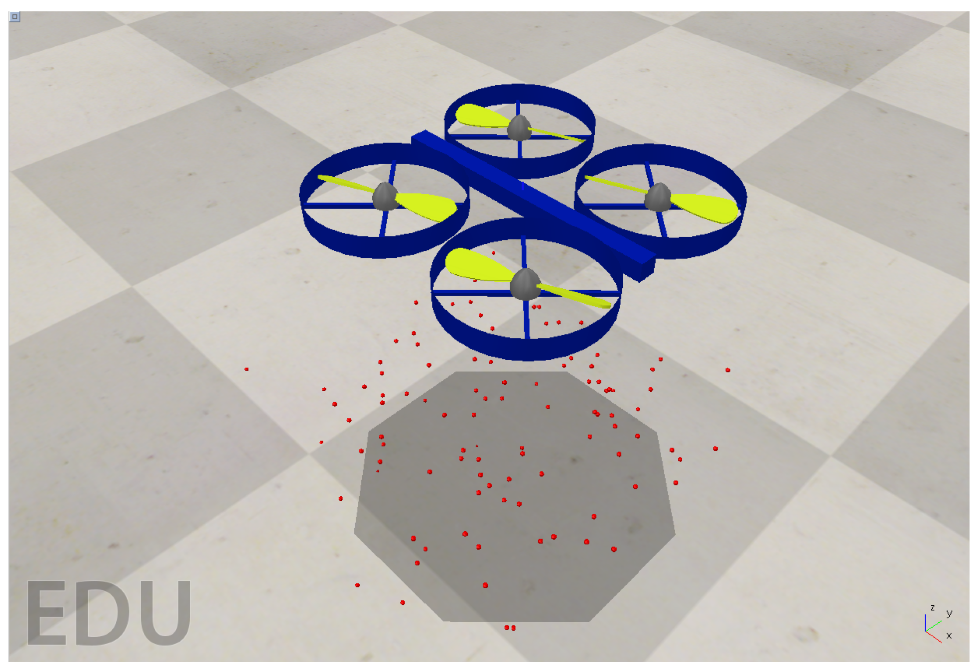
The simulation of the unknown system, in this case a quadrotor as shown in Figure 4, is carried out exclusively in CoppeliaSim, where position and trajectory results are obtained. Conversely, the trajectory inference algorithm is implemented in MATLAB^®/Simulink^® (version R2026a).

6.1. Trajectory Inference—Position Control

The gains used in the simulation of the unknown system are The gains considered for the trajectory control are $k_p^x=0.1$, $k_v^x=0.05$, $k_p^{\theta }=1.0$, $k_d^{\theta }=0.15$, $k_p^y=0.1$, $k_v^y=0.05$, $k_p^{\varphi }=1.0$, $k_d^{\varphi }=0.15$, $k_p^z=150$, $k_v^z=8.0$, $k_p^{\psi }=140$, and $k_d^{\psi }=12.01$. It is emphasized that these gains belong to the stabilizing controller of the quadrotor, treated throughout this work as the unknown system whose trajectory is to be inferred; as such, knowledge of the specific gain values or the tuning method used to obtain them is neither required nor exploited by the trajectory inference scheme.

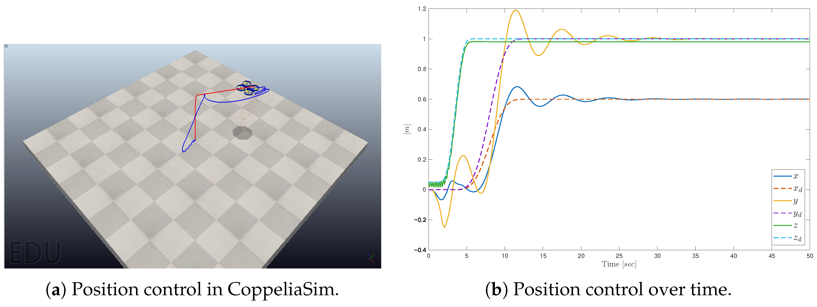
The quadrotor’s initial condition was ${\left[000000000000\right]}^{\top }$, while the desired yaw angle remains ${\psi }^{\ast }=0$ throughout the entire simulation. For the trajectory inference case under position control, the simulation is carried out over 50 s as illustrated in Figure 5. Specifically, in Figure 5a, the position control in CoppeliaSim is shown, where the desired trajectory is depicted in red and the trajectory described by the quadrotor in blue. The system is evidently affected by disturbances, which are:

$$\begin{array}{cc}\hfill d_x& =0.02sin\left(1.2t\right)+0.01cos\left(0.2t\right)d_{\theta }=0.01sin\left(0.2t\right)\hfill \\ \hfill d_y& =0.02sin\left(0.2t\right)d_{\varphi }=0.01sin\left(1.04t\right)+0.01cos\left(0.03t\right)\hfill \\ \hfill d_z& =0.3sin\left(1.2t\right)+0.01cos\left(0.2t\right)d_{\psi }=0.01cos\left(0.001t\right)\hfill \end{array}$$

These disturbance signals are deterministic and additive; no additional random noise was explicitly injected into the simulation. It is noted, however, that the CoppeliaSim physics engine (Bullet Physics 2.78) also introduces an additional, implicit fluctuation, likewise additive, through its particle-based propeller-thrust model.

The matrix $\Gamma$ is set to $400I_{28}$. For the CLOE-SM algorithm, the gains employed are those reported in

Table 1. Gains for trajectory control case.

Block	Gain	Value
${\mathsf{\Sigma }}_{x-\theta }$	${\alpha }_{11}$	0.12
	${\alpha }_{12}$	0.18
	${\alpha }_{13}$	0.24
	${\alpha }_{14}$	0.3
${\mathsf{\Sigma }}_{y-\varphi }$	${\alpha }_{11}$	0.12
	${\alpha }_{12}$	0.18
	${\alpha }_{13}$	0.24
	${\alpha }_{14}$	0.3
${\mathsf{\Sigma }}_z$	${\alpha }_{11}$	0.24
	${\alpha }_{12}$	0.3
${\mathsf{\Sigma }}_{\psi }$	${\alpha }_{11}$	0.24
	${\alpha }_{12}$	0.3

. The desired position references for x, y, and z were defined as smooth interpolating polynomials. $x_d$ rises from 0 to $0.6$ m over the interval $[4.0,13.4]$ s; $y_d$ transitions from 0 to $1.0$ m over the same interval $[4.0,13.4]$ s; and $z_d$ ascends from $0.05$ to $1.0$ m over the interval $[1.0,3.0]$ s, after which, all references remain constant at their final values.

6.1.1. Disturbance-Free Case

This subsection presents the comparative results between the CLOE and CLOE-SM algorithms under the trajectory inference scenario without disturbances, in order to isolate and evaluate the contribution of the sliding-mode correction term on the estimation performance.

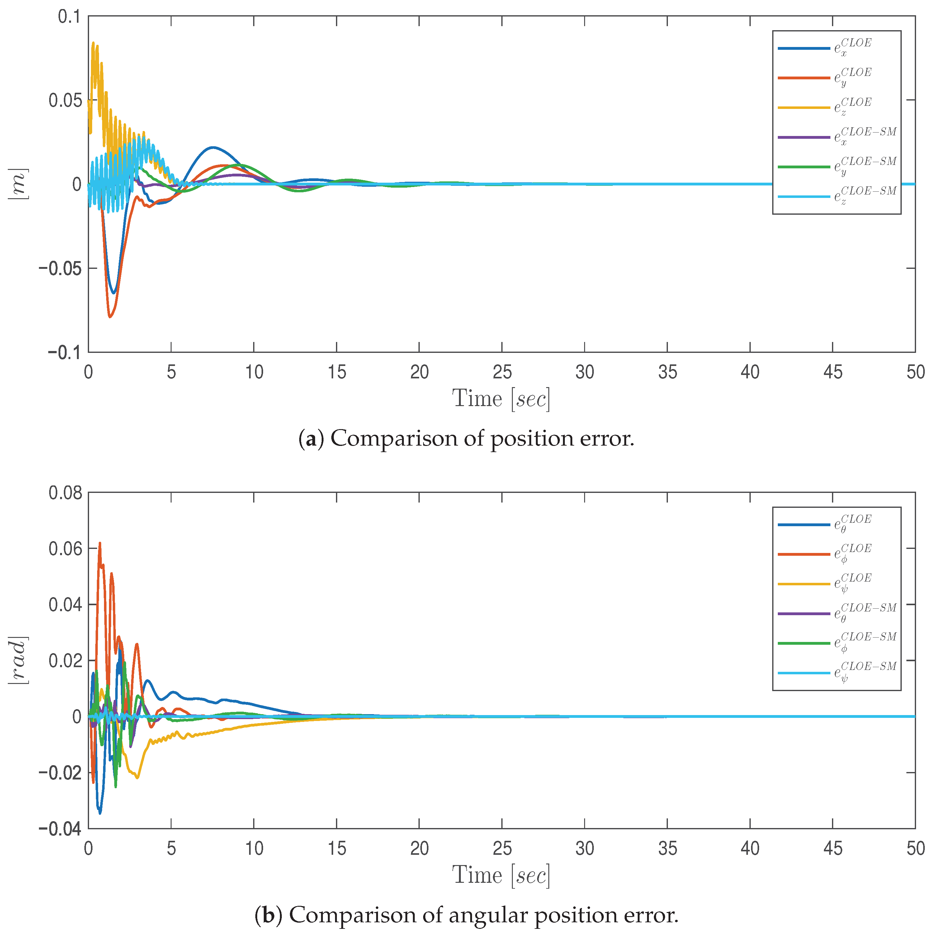
Figure 6a presents a comparison of the estimation errors for the position states x, y, and z between the CLOE and CLOE-SM algorithms. It can be observed that the CLOE-SM algorithm yields a notably faster estimation error convergence relative to the CLOE algorithm, demonstrating the effectiveness of the sliding-mode correction term in improving the estimation accuracy. Figure 6b presents a comparison of the estimation errors corresponding to $\theta$, $\varphi$, and $\psi$. It can be observed that the CLOE-SM algorithm achieves a notably faster convergence of the error toward zero relative to the CLOE algorithm.

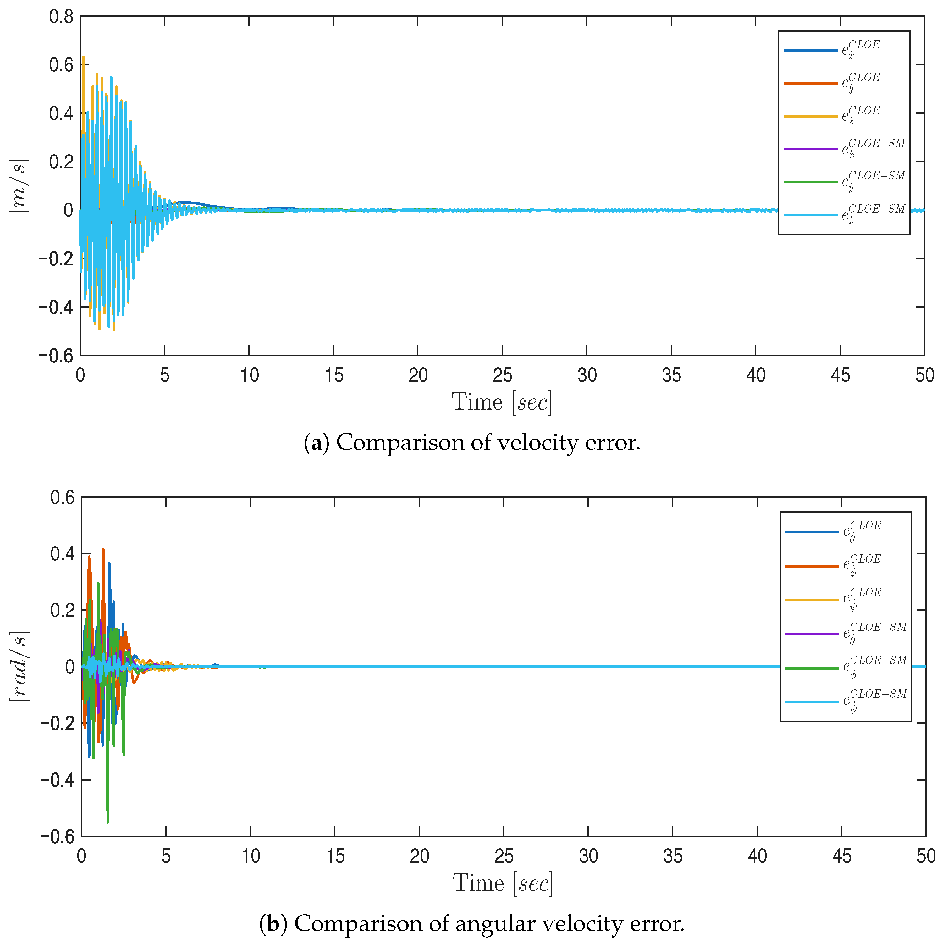
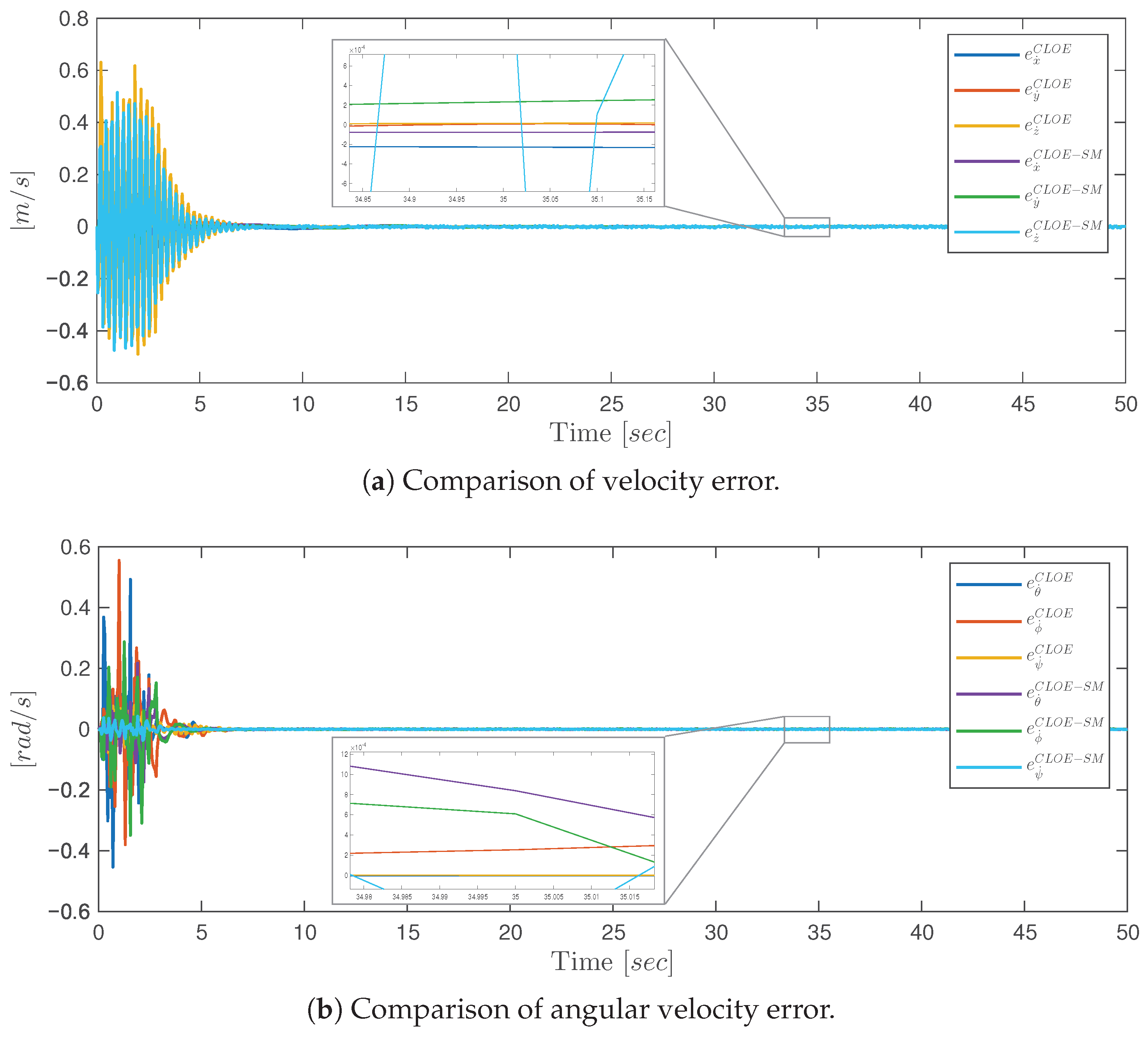
Similarly, Figure 7a shows the estimation errors for the velocity states $\dot{x}$, $\dot{y}$, and $\dot{z}$ under both algorithms. As in the previous case, the CLOE-SM algorithm exhibits a markedly faster convergence rate compared to CLOE, further confirming the benefit of incorporating the sliding-mode correction term. Figure 7b presents the corresponding comparison for the angular velocity errors $\dot{\theta }$, $\dot{\varphi }$, and $\dot{\psi }$, where the same improvement in convergence speed is observed for the CLOE-SM scheme relative to CLOE.

6.1.2. Disturbance Case

This subsection presents the comparative results between the CLOE and CLOE-SM algorithms under the trajectory inference scenario in the presence of disturbances, in order to evaluate the robustness and effectiveness of the sliding-mode correction term under a more challenging and realistic operating condition.

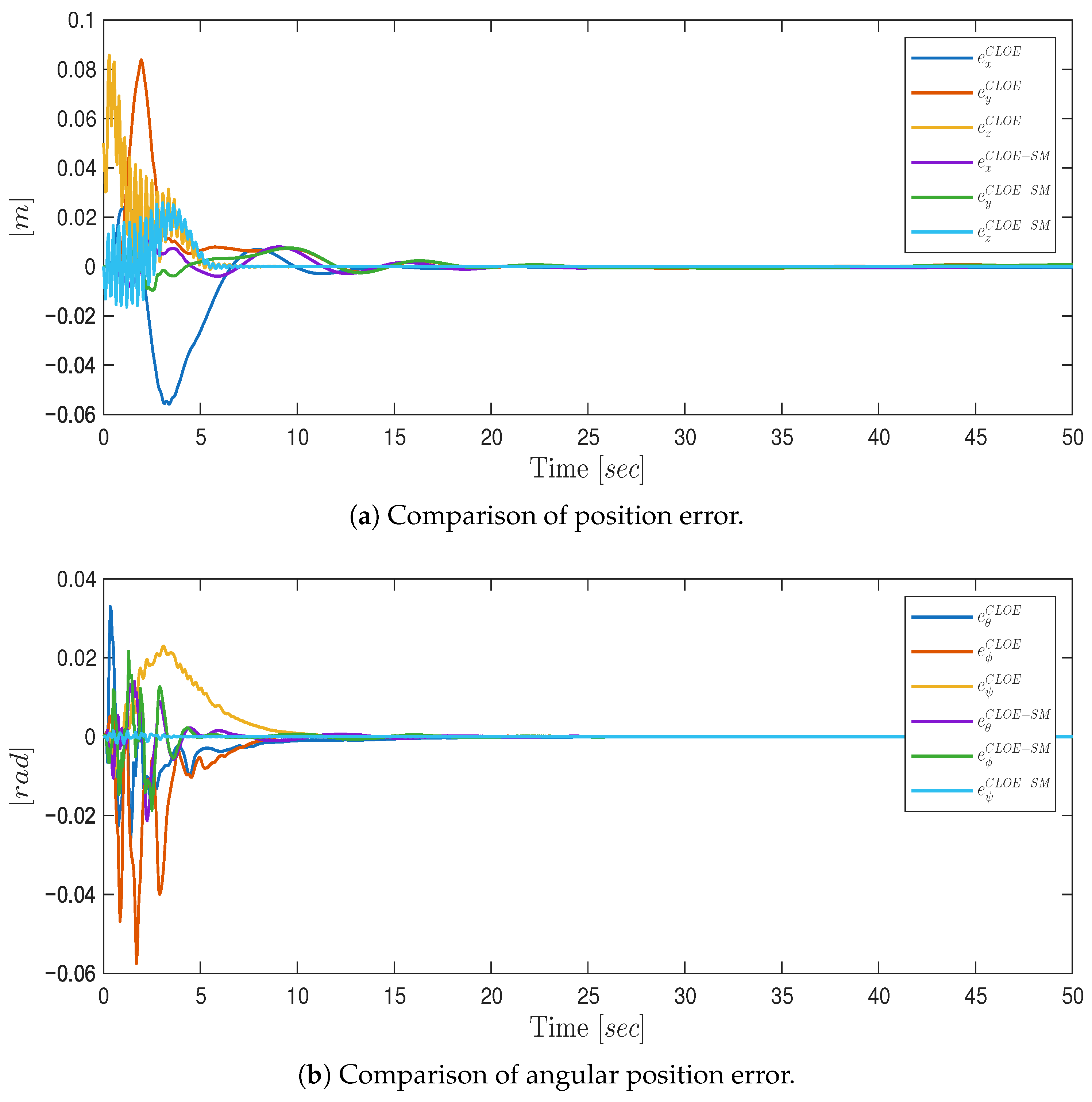
Figure 8a shows the estimation errors for the position states x, y, and z obtained with the CLOE and CLOE-SM algorithms under the disturbance scenario. Despite the presence of external disturbances, the CLOE-SM algorithm maintains a substantially faster convergence rate than CLOE, confirming the robustness of the sliding-mode correction term against unmodeled dynamics. Figure 8b presents the corresponding results for the attitude states $\theta$, $\varphi$, and $\psi$, where the CLOE-SM algorithm again exhibits superior convergence performance relative to CLOE under the same disturbance conditions.

As shown in the magnified view in Figure 9, around $t=35\mathrm{s}$ the position estimation error remains on the order of ${10}^{-4}\mathrm{m}/\mathrm{s}$, while the attitude estimation error remains on the order of ${10}^{-3}\mathrm{rad}/\mathrm{s}$, illustrating the sustained accuracy of the CLOE-SM scheme despite the persistent disturbance. It is worth noting that the chattering phenomenon associated with the discontinuous correction terms was mitigated to the greatest extent possible through the appropriate selection of the sliding-mode gains, in accordance with the conditions established in Theorem 2.

6.1.3. Quantitave Performance

To quantitatively compare the results obtained, the Root Mean Square Error (RMSE) were calculated as follows

$$\begin{array}{c}\hfill v^{\mathrm{RMSE}}=\sqrt{{\displaystyle \frac{1}{n}}{\displaystyle \sum _{i=1}^n}{e}^2\left(t\right)}.\end{array}$$

(57)

The RMSE is employed to quantitatively assess the performance of both algorithms considering the case with disturbances, with the results summarized in

Table 2. $RMSE$ norm for the case position control.

Algorithm	Value
CLOE	0.519
CLOE-SM	0.367

. As observed, the CLOE-SM algorithm yields a lower RMSE norm value of $0.367$, compared to $0.519$ obtained by the CLOE algorithm, indicating a superior performance metric under this criterion. This improvement is primarily attributed to the sliding-mode correction term, which enforces a faster and more aggressive drive of the estimation error toward zero, thereby reducing the overall RMSE despite the inherent chattering effect. These results demonstrate that the CLOE-SM algorithm outperforms CLOE both in terms of convergence rate and accumulated estimation error.

To quantitatively compare the results obtained, the Integral of Time-weighted Absolute Error (ITAE) was calculated as follows

$$\begin{array}{c}\hfill v^{\mathrm{ITAE}}={\int }_0^{T}t·\parallel \mathbf{e}\left(t\right)\parallel dt,\end{array}$$

(58)

where T is the total simulation time, t is the time variable, and $\parallel \mathbf{e}\left(t\right)\parallel$ denotes the Euclidean norm of the inference error vector for each subsystem.

Table 3. ITAE performance metric—Position inference.

Subsystem	CLOE	CLOE-SM
Position $(x,y,z)$	0.983	0.58
Velocity $(\dot{x},\dot{y},\dot{z})$	1.946	1.378
Euler angles $(\theta ,\varphi ,\psi )$	0.594	0.105
Angular rates $(\dot{\theta },\dot{\varphi },\dot{\psi })$	1.05	1.24

presents the ITAE metric for the position inference case. The proposed CLOE-SM algorithm achieves superior performance for the position, velocity, and Euler angle subsystems. For the position subsystem, CLOE-SM yields an ITAE value of $0.58$ compared to $0.983$ for CLOE, representing an improvement of approximately $41\%$. Likewise, the velocity subsystem shows a reduction from $1.946$ to $1.378$, corresponding to an improvement of $29\%$. The most notable improvement is observed for the Euler angles subsystem, where CLOE-SM reduces the ITAE value from $0.594$ to $0.105$, an improvement of approximately $82\%$. In contrast, for the angular rates subsystem, CLOE slightly outperforms CLOE-SM, yielding a lower ITAE value of $1.05$ compared to $1.24$, an increase of approximately $18\%$. This result is attributed to the chattering effect introduced by the discontinuous terms of the sliding-mode-based observer, which affects the angular rate channels more noticeably than the remaining subsystems. Overall, these results indicate that the sliding-mode correction term incorporated in CLOE-SM contributes to a faster convergence of the inference error for the position, velocity, and orientation states, at the expense of a slight performance degradation in the angular rate estimation due to the aforementioned chattering effect. It is worth noting that this marginal degradation in the angular rate subsystem stems from the gain tuning of $\Lambda$. The gains for the angular rate channels were therefore selected as a trade-off between chattering attenuation and disturbance rejection, which explains the slightly larger ITAE value obtained by CLOE-SM relative to CLOE in this particular subsystem.

6.1.4. Identified Parameters

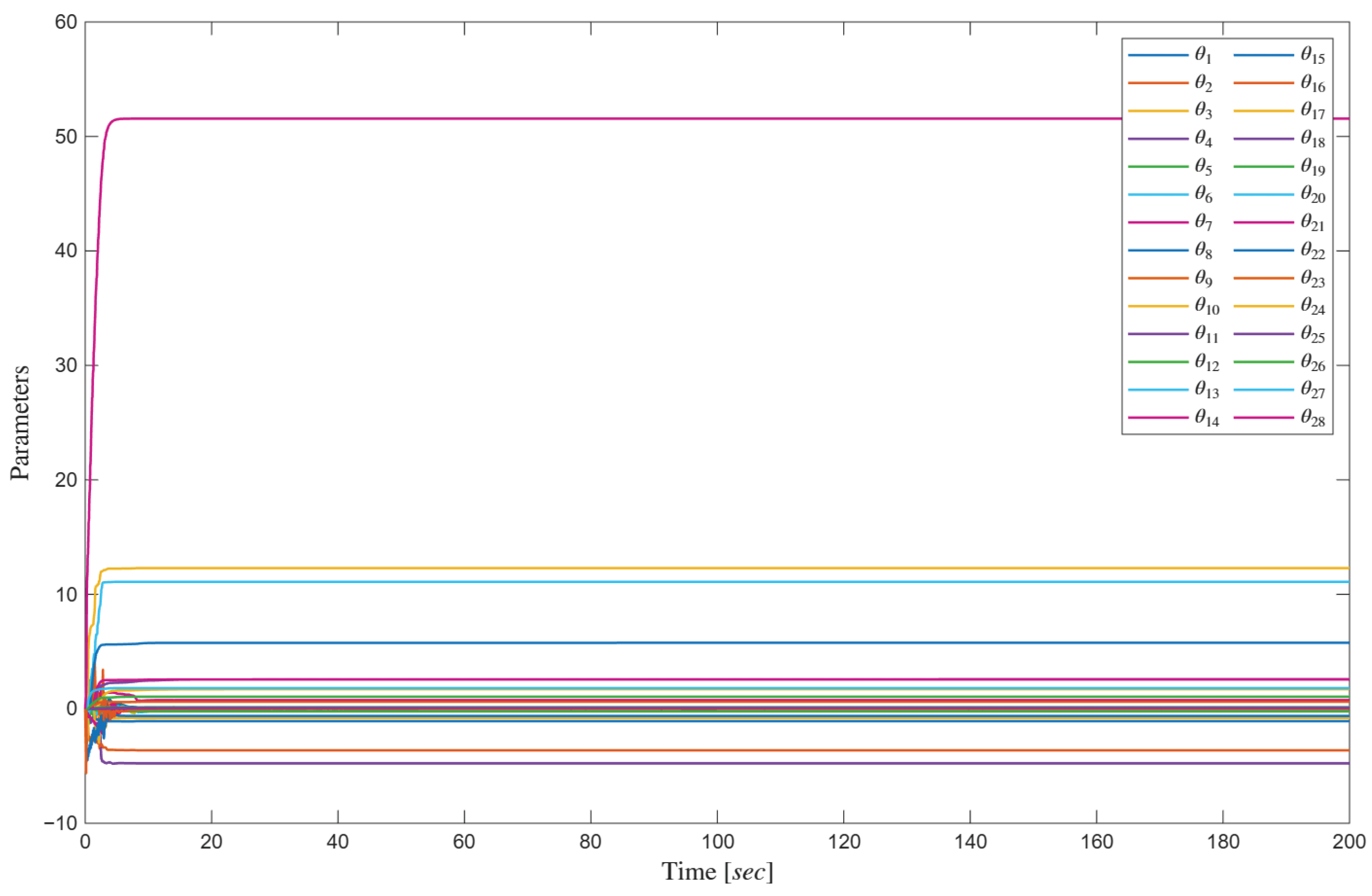
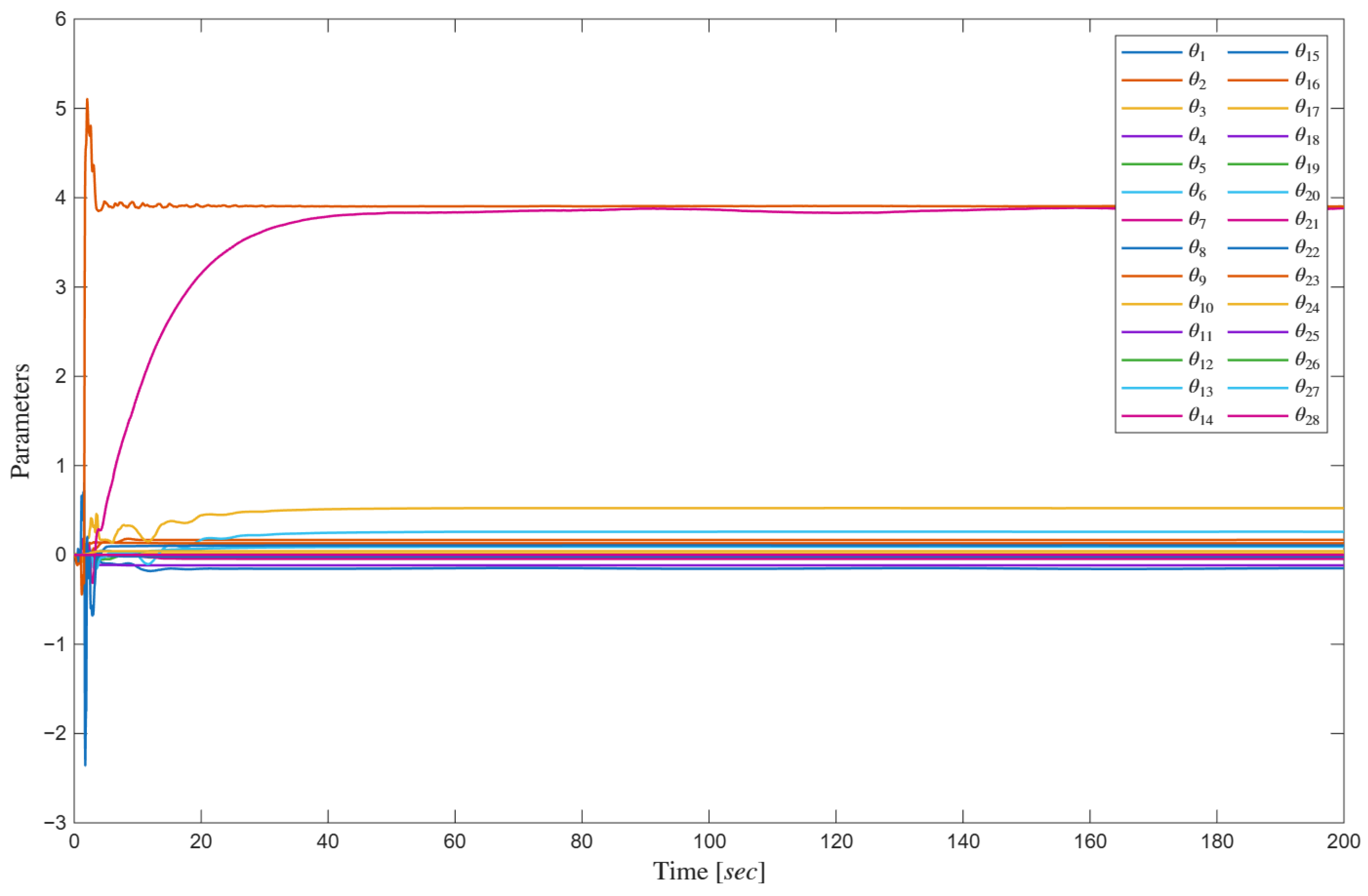
In order to show the convergence of the parameters, the simulation time was extended to 200 s. Figure 10 shows the parameters for the CLOE algorithm. The convergence to constant values of the 28 parameters ($A_c,B_c$ and gain $\mathcal{L}$) is observed.

Similarly, Figure 11 illustrates the parameter convergence of the CLOE-SM algorithm for all 28 estimated parameters. In this case, only one parameter exhibits a slightly oscillatory behavior, which is attributed to the discontinuous nature of the sliding-mode correction term. Nevertheless, this parameter, as well as the others, remains bounded throughout the estimation process.

6.2. Trajectory Inference—Trajectory Control

Another case to validate inference trajectory robust algorithm is through implementation of a trajectory control of the unknown system. In that sense, the proposed desired trajectory has the following form:

$$\begin{array}{cc}\hfill x_d=& 1.6sin\left(wt\right)m,z_d=1m,\hfill \end{array}$$

(59)

$$\begin{array}{cc}\hfill y_d=& 3.0sin\left(wt\right)cos\left(wt\right)m,{\psi }_d=pi/16rad\hfill \end{array}$$

(60)

where w is a frequency of 0.03.

For the trajectory-control case, the simulation runs for 140 s to complete a full cycle of the desired trajectory. The same gains reported for position case and in Table 1 are used, along with the same values of the matrix $\Gamma$.

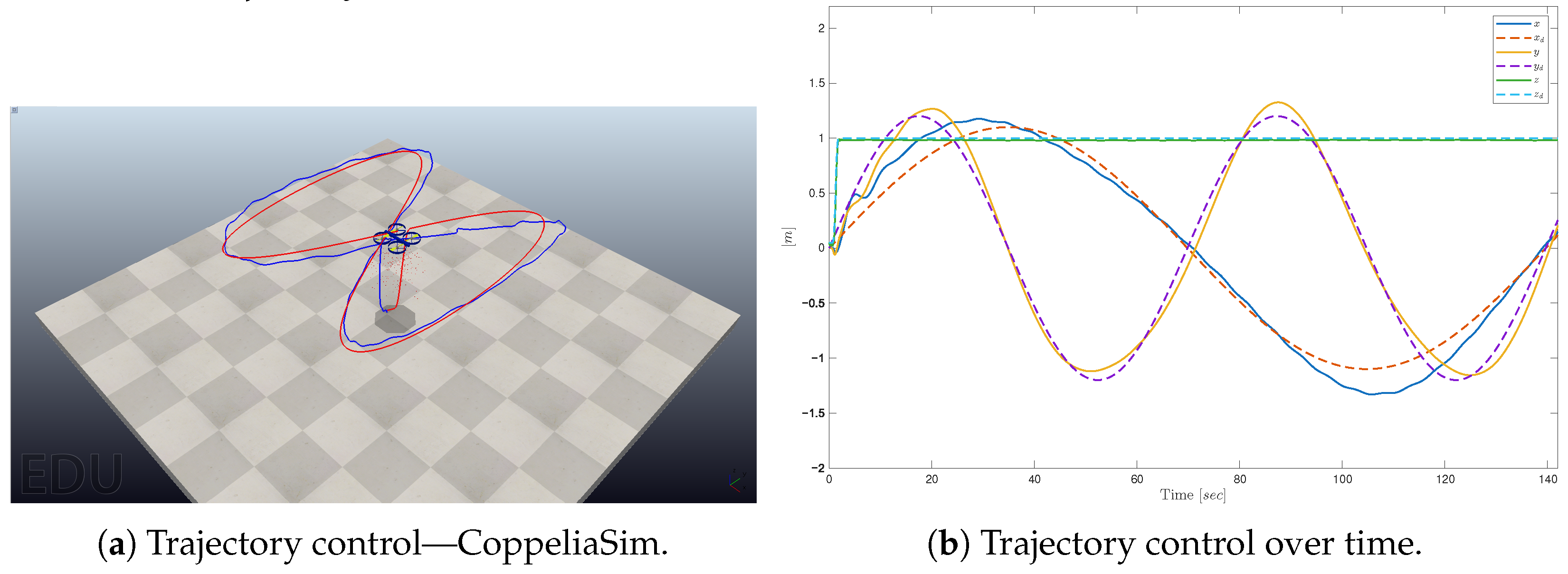
Figure 12 illustrates trajectory control of the quadrotor, specifically in Figure 12a, we can see the trajectory control in the CoppeliaSim environment where we have the desired trajectory in red and the trajectory described by the quadrotor in blue. In Figure 12b, we can see the trajectory control over the time.

For the sake of conciseness, only the performance metrics are reported for the trajectory-tracking case, since the qualitative behavior of the estimation errors and parameter convergence closely follows the same trends already illustrated in detail for the position control case.

$RMSE$ is employed to quantitatively evaluate the performance of both algorithms during trajectory tracking, with the results summarized in

Table 4. $RMSE$ for the case trajectory control.

Algorithm	Value
CLOE	0.58
CLOE-SM	0.42

. In this case, the CLOE-SM algorithm achieves a notably lower $RMSE$ value of $0.42$ compared to $0.58$ obtained by CLOE, representing an improvement of approximately $28\%$. This result further confirms that the sliding-mode correction term incorporated in CLOE-SM effectively drives the estimation error toward zero at a faster rate, outperforming CLOE both in terms of convergence speed and accumulated estimation error throughout the simulation.

Table 5. ITAE performance metric—Trajectory inference.

Subsystem	CLOE	CLOE-SM
Position $(x,y,z)$	14.567	11.51
Velocity $(\dot{x},\dot{y},\dot{z})$	17.17	15.05
Euler angles $(\theta ,\varphi ,\psi )$	5.534	5.027
Angular rates $(\dot{\theta },\dot{\varphi },\dot{\psi })$	3.278	2.91

summarizes the ITAE metric for the trajectory-inference case. The CLOE-SM algorithm demonstrates superior performance across all subsystems. For the position subsystem, CLOE-SM achieves an ITAE value of $11.51$ compared to $14.567$ for CLOE, representing an improvement of approximately $21\%$. For the velocity subsystem, CLOE-SM yields a value of $15.05$ compared to $17.17$ obtained by CLOE, corresponding to an improvement of approximately $12\%$. The Euler angles subsystem also shows a modest improvement, with CLOE-SM reducing the ITAE value from $5.534$ to $5.027$, a reduction of approximately $9\%$. Finally, for the angular rates subsystem, CLOE-SM achieves a value of $2.91$ compared to $3.278$ for CLOE, representing an improvement of approximately $11\%$. These results consistently confirm that the sliding-mode correction term incorporated in CLOE-SM contributes to a faster convergence of the inference error across all subsystems throughout the trajectory tracking simulation, with the most notable improvement observed in the position subsystem.

Based on the performance metrics, namely the RMSE and the ITAE, as well as the qualitative assessment of the parameter convergence plots, both proposed schemes demonstrate a progressive reduction in tracking error and parameter convergence over time, with the CLOE-SM approach exhibiting superior performance in terms of estimation accuracy and convergence speed. These results are consistent with the theoretical guarantees established in Theorems 1 and 2, where the uniform ultimate boundedness of the estimation error is formally proven, and further confirm that a careful selection of the sliding-mode gains, following the channel-wise dominance condition derived therein, effectively mitigates the chattering effect while preserving the improved convergence performance of the CLOE-SM scheme.

It is worth noting that, beyond the deterministic disturbances defined in Section 3, the CoppeliaSim physics engine (Bullet Physics 2.78) introduces an additional, implicit source of non-deterministic-like uncertainty: propeller thrust is generated through a particle-based air-flow model, in which the position, direction, and velocity of the simulated air particles are subject to pseudo-random disturbances, thereby inducing a small-amplitude stochastic fluctuation in the commanded thrust. Nevertheless, the proposed trajectory-inference scheme remains robust to bounded disturbances irrespective of their deterministic or stochastic origin, since the inference design relies solely on the disturbance bound rather than its specific nature. Consistent with this, the inference tracking error metrics reported throughout this section indicate that neither the tracking behavior of the unknown system nor the trajectory inference are noticeably affected by this additional source of disturbance, thereby supporting the robustness of the proposed scheme under realistic, non-idealized simulation conditions.

7. Conclusions

This manuscript introduces the CLOE-SM algorithm for trajectory inference of quadrotor UAVs, which incorporates a high-order sliding-mode observer to enhance the robustness of the estimation scheme. The proposed algorithm is evaluated and compared against the CLOE algorithm under position regulation and trajectory-following scenarios, with all simulations carried out in the CoppeliaSim robotics environment. Both algorithms achieved convergence of the estimation errors to small bounded values, with CLOE-SM attaining finite-time convergence due to the integration of sliding-mode correction terms. Regarding parameter estimation, both algorithms converged to stable values, sufficient to ensure precise state estimation throughout the experiments.

In terms of estimation performance, both the RMSE and ITAE metrics consistently indicate that the CLOE-SM algorithm outperforms CLOE in both evaluated scenarios. Overall, these results demonstrate that the sliding-mode correction term effectively enhances the convergence behavior of the inference error, consolidating CLOE-SM as a robust alternative for trajectory inference of quadrotor UAVs under both position regulation and trajectory tracking conditions.

Future work will address the trajectory-inference problem considering only partial state measurements. Furthermore, the robustness of the proposed CLOE-based framework will be further investigated under more complex disturbance scenarios, and the methodology will be validated through real flight experiments on a physical quadrotor platform.