1. Introduction
With the growing demand for efficient and long-endurance solutions in monitoring, surveying and logistical operations, solar-powered unmanned aerial vehicles (UAVs) have emerged as a significant advancement in aerospace technology [
1,
2,
3,
4]. By converting incident sunlight into electrical energy and storing the surplus on board, these aircraft offer the prospect of prolonged flight without traditional refuelling [
3]. Their extended endurance makes them especially valuable for environmental monitoring, search-and-rescue missions, exploration of uncharted regions and the provision of communication services in remote areas [
1,
2].
1.1. Motivation
The operational independence and low logistical footprint of solar-powered UAVs make them ideal candidates for missions where conventional propulsion systems or fuel supplies are limiting—particularly missions requiring a persistent aerial presence or coverage of remote and difficult-to-access regions [
2]. However, their performance remains highly dependent on a wide range of technical and environmental factors—altitude, solar irradiance, panel orientation, battery capacity and atmospheric conditions—all of which interact in complex ways to determine the overall energy balance. A detailed, quantitative understanding of these interactions is essential for designing UAVs that can approach near-perpetual endurance under real-world constraints [
2,
3].
1.2. Literature Review
Existing research has addressed many facets of solar-UAV performance. Early work on autonomous solar flight established the core design principles for continuous operation [
3], and comprehensive studies have since demonstrated multi-day endurance with compact, hand-launchable platforms, culminating in the 81 h AtlantikSolar flight [
4,
5]. Propulsion-system testing for long-endurance solar aircraft [
6] and parameter-determination methods for high-altitude long-endurance (HALE) concepts [
7,
8] have refined the sizing toolset, while configuration-level optimisation studies—genetic-algorithm and priority-based formulations—have explored the structural and energy trade-offs of low- and high-altitude designs [
9,
10]. In parallel, a substantial body of work addresses energy-optimal trajectory planning and power management, from perpetual-endurance path planning [
11,
12] to mission-profile-aware power management [
13].
Two limitations recur across this literature. First, most endurance models remain strongly context-dependent: they are tied to a specific platform or a specific altitude band and are not readily transferable across mission profiles. Second, and more specific to the present work, the conversion from incident irradiance to collected electrical power is almost universally treated with a flat-plate assumption—the photovoltaic array is modelled as a horizontal panel of equivalent area [
3,
7,
14]. Real solar UAVs carry their cells on a cambered, dihedralled, often tapered wing, and the orientation of those cells relative to the sun depends on the aircraft heading. The flat-plate assumption therefore discards both the heading dependence of collection and the geometric gain or loss introduced by the wing shape itself. Recent photovoltaic-modelling studies confirm that surface curvature and the resulting non-uniform illumination materially affect the power output of curved aerial arrays [
15,
16], reinforcing the case for a geometry-resolved collection model in place of the flat-plate idealisation. The present study builds on these foundations by introducing a configurable energy-simulation framework intended for rapid design iteration and scenario testing and by replacing the flat-plate assumption with an explicit, closed-form wing-geometry collection model. Where prior frameworks represent the array either as a horizontal panel of equivalent area [
3,
7,
14] or through a tabulated incidence factor evaluated numerically at each step, the present model condenses the entire surface geometry into three scalars and an analytic closed form (Equation (19)), giving the collected power at any sun position and heading without per-step mesh integration and admitting an exact orbit-average for circular loiter—a level of analytical transparency not available in the existing flat-plate or look-up approaches.
1.3. Contribution and Scope
The primary objective of this study is to develop and validate an energy-simulation framework tailored to solar-powered UAVs, with emphasis on guiding their design and estimating operational feasibility for long-duration missions. The framework makes three contributions. First, it couples a physics-based environmental irradiance model—astronomical solar position, broadband atmospheric transmission scaled by air mass and altitude and an eccentricity-corrected extraterrestrial reference—with the energy-balance computation, so that the same tool is applicable from sea level to the stratosphere. Second, it introduces a wing-geometry photovoltaic collection model that reduces an arbitrary cambered wing to three scalar coefficients and yields a closed-form expression for collected power as a function of sun position and aircraft heading, together with an exact orbit-averaging result for circular loiter. Third, the framework is validated against a ground-based testing campaign conducted on a real solar-UAV demonstrator—the Aurora aircraft—instrumented with a bespoke onboard energy-monitoring unit.
Unlike previous works that focus either on low-altitude optimisation or on platform-specific test campaigns, the framework presented here is general purpose, modular and altitude independent and is explicitly anchored to flight-representative hardware. It bridges the gap between experimental insight and early-phase design needs, providing a lightweight yet physically faithful tool for feasibility screening.
1.4. Document Structure
The remainder of this paper is organised as follows.
Section 2 introduces the operational context and the technical and environmental factors that govern solar-UAV endurance.
Section 3 develops the methodology: the simulation concept, the environmental irradiance model, the wing-geometry collection model, the energy-balance computation, the software implementation and analysis modes and the Aurora experimental platform.
Section 4 presents the simulation results across single-day, annual and global scopes and reports the validation of the solar power-generation model against the Aurora charging campaign.
Section 5 discusses the findings, limitations and future extensions, and
Section 6 concludes.
3. Methods
To determine the endurance—or the feasibility of continuous flight—under a given set of conditions, it is necessary to simulate the aircraft’s energy balance over the entire flight. The energy balance relates the available onboard energy to the aircraft’s energy demand. The available energy depends on the capacity of the onboard battery and on the ability to recharge it from the solar array; the propulsion system is typically the largest consumer, but all onboard systems must also be accounted for.
3.1. Simulation Concept
The simulation uses a time-stepped approach that tracks the battery state of charge (SoC) by evaluating, at each time interval, the difference between incoming solar energy and the aircraft’s power consumption. From the input parameters—geographic position, date, altitude, battery capacity, photovoltaic configuration and power demand—the model computes the solar position, estimates the collected power and updates the SoC, thereby determining whether the UAV can sustain continuous operation under the specified conditions. The framework integrates three coupled sub-models, evaluated in sequence at every step:
Environmental irradiance model—determines the solar position and the direct normal irradiance at the platform from astronomical and atmospheric inputs (
Section 3.2).
Wing-geometry collection model—maps the incident irradiance to the electrical power produced by photovoltaic cells distributed over the curved wing surface, accounting for the aircraft heading (
Section 3.3).
Energy-balance model—updates the battery SoC over time by subtracting consumption and adding generated power (
Section 3.4).
By iterating these steps in short increments, the simulation predicts when energy reserves are sufficient for continuous flight and when they fall below critical thresholds.
3.2. Environmental Irradiance Model
The environmental irradiance model computes the solar vector and the direct normal irradiance at the platform from astronomical and atmospheric inputs. Its two outputs—the unit solar vector in the local horizontal frame and the direct normal irradiance—feed the wing-geometry collection model of
Section 3.3.
3.2.1. Solar Position
The solar position at latitude φ, longitude λ and instant t is computed from standard astronomical relations [
28]. The solar declination is approximated by Cooper’s formula [
29]:
where
is the day of the year. The local apparent solar time corrects local clock time for the longitude offset from the time-zone meridian and for the equation of time EoT, evaluated from Spencer’s Fourier-series approximation [
30]:
and the hour angle, the angular distance of the sun from the local meridian, is
The solar elevation angle α above the local horizon follows from the spherical-trigonometric identity [
31]
and the solar azimuth A, measured clockwise from north, from [
32]
with the convention
A → 360° −
A in the afternoon. The unit solar vector in the local horizontal frame, with components ordered east, north and up, is then
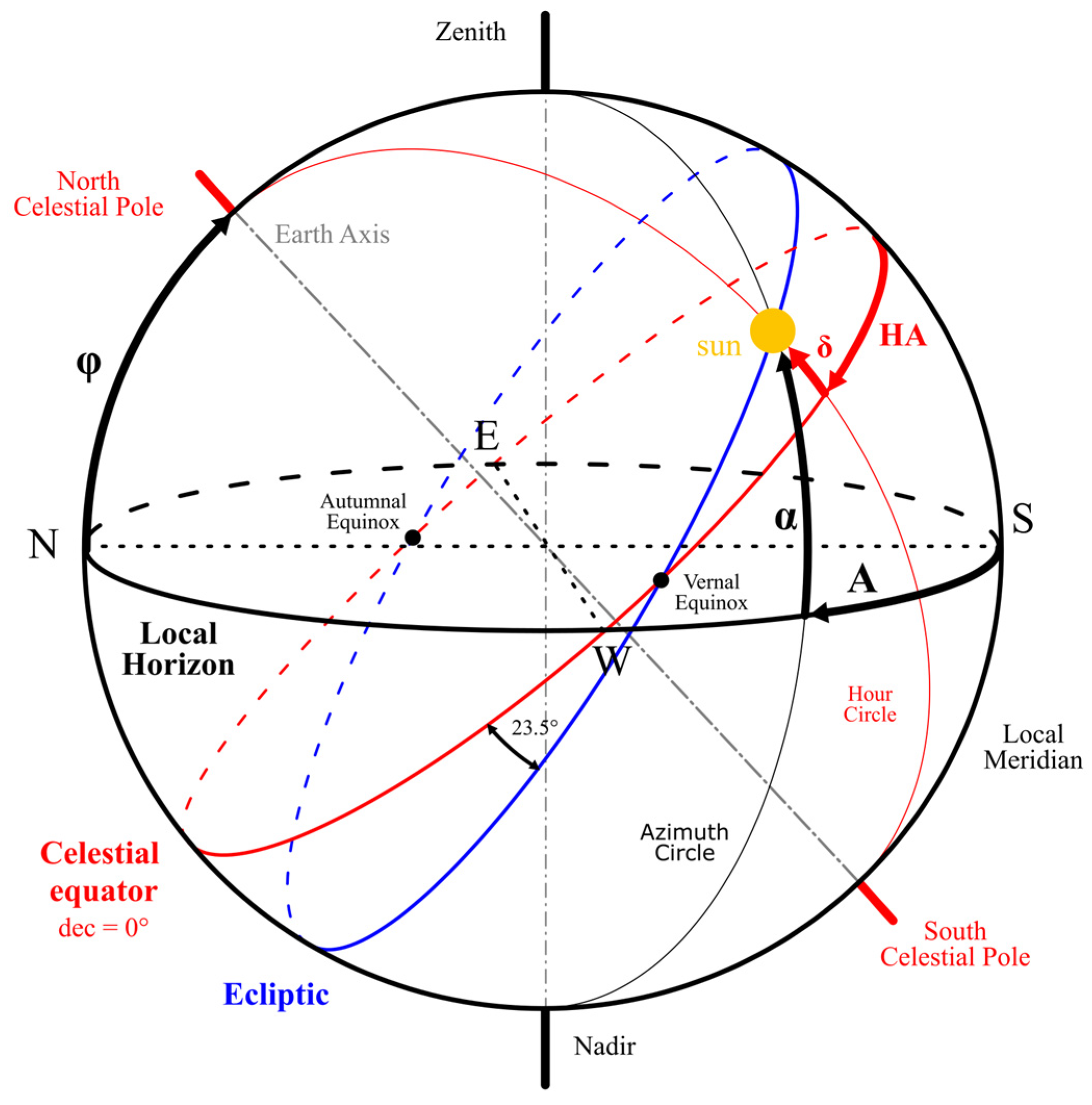
The geometric relationships among declination, hour angle, observer latitude and the resulting elevation and azimuth are illustrated in
Figure 1.
3.2.2. Extraterrestrial Irradiance and Atmospheric Attenuation
The direct normal irradiance at the top of the atmosphere is the solar constant adjusted for the eccentricity of the Earth–Sun orbit:
with the mean solar constant taken as
, the current total-solar-irradiance estimate [
27]. The eccentricity correction produces a ±3.3% seasonal variation between perihelion in early January and aphelion in early July. The fraction of
that reaches the platform after passage through the residual atmosphere above it is captured by a broadband transmission coefficient [
33]:
where
τ0 ≈ 0.70 is the clear-sky transmission at sea level with the sun overhead,
AM is the relative air mass at the platform’s solar elevation and
p/
p0 is the pressure ratio between platform altitude and sea level. Both factors represent the geometric path length of the beam through the absorbing and scattering atmosphere. The relative air mass is computed with the Kasten–Young formula [
34]
which reduces to the familiar
approximation at high elevation and remains finite at the horizon, where the simpler form diverges unphysically. The pressure ratio is evaluated from the U.S. Standard Atmosphere [
35], represented as a linear-lapse-rate troposphere up to 11 km:
with
L the tropospheric lapse rate,
T0 the sea-level temperature and
gM/(
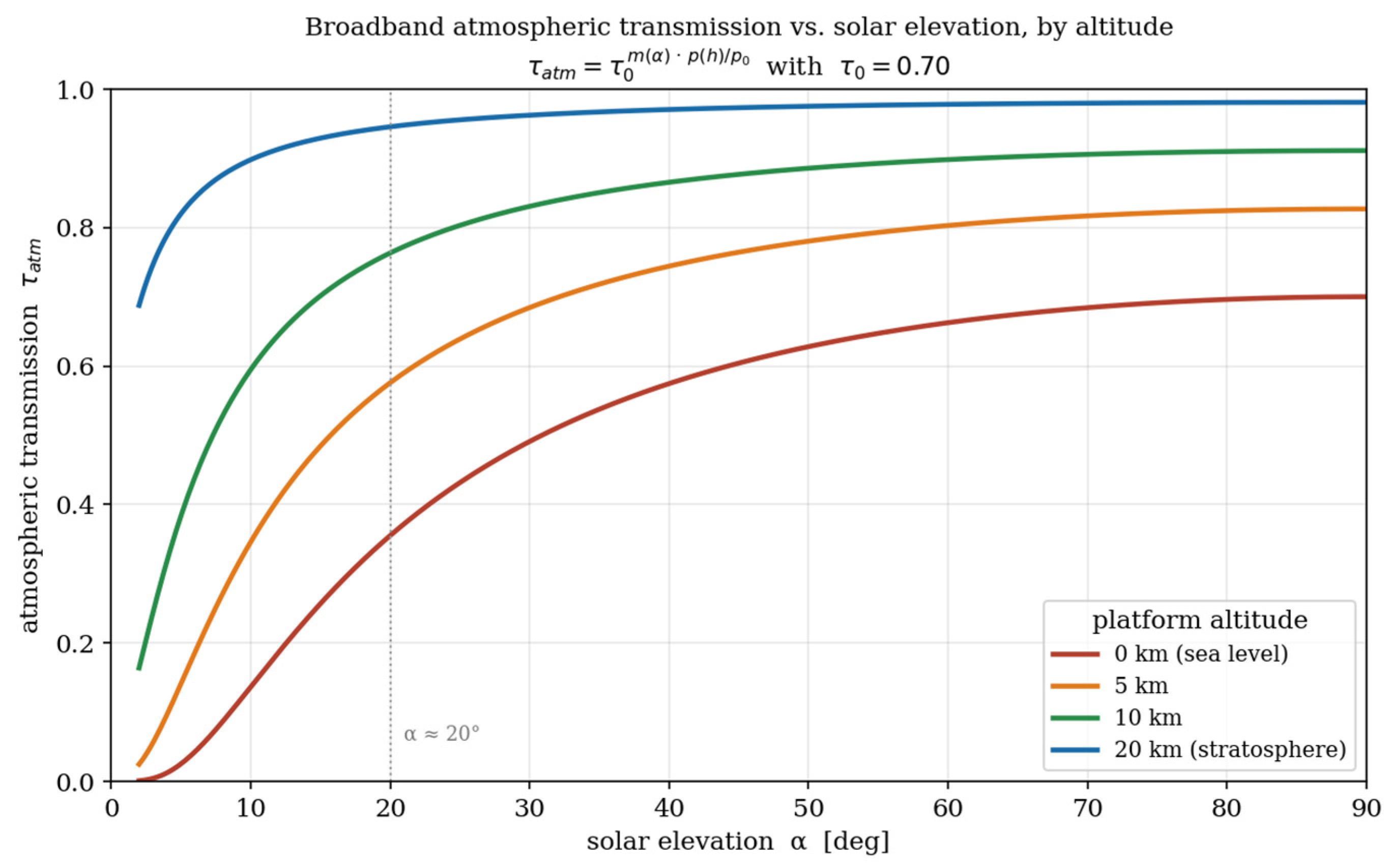
RL) the lapse-rate exponent; above 11 km, the isothermal-layer relation is used. For stratospheric operation, the pressure ratio falls by more than an order of magnitude relative to sea level, reducing the air-mass–pressure product and driving
kA toward unity. This captures the principal physical advantage of high-altitude flight: the platform operates above most of the absorbing column. The behaviour of the transmission coefficient with solar elevation and altitude is shown in
Figure 2.
Cloud cover further reduces the irradiance through a cloud attenuation coefficient
, where
corresponds to clear sky. For stratospheric operation above the cloud-bearing troposphere,
is used throughout; for tropospheric operation, it is a configurable input that may be set from observation or forecast. Combining the three factors, the direct normal irradiance at the platform is
which is the irradiance falling on a surface oriented normal to the solar vector. The horizontal flat-panel reference irradiance, used in earlier conceptual studies and forming the baseline against which the curved-wing collection coefficient is defined, is recovered directly:
Three assumptions bound the validity of the irradiance model and are stated explicitly. First, only the direct-beam component is treated; diffuse irradiance is small at stratospheric altitude (a few percent) and is omitted, an established and conservative simplification [
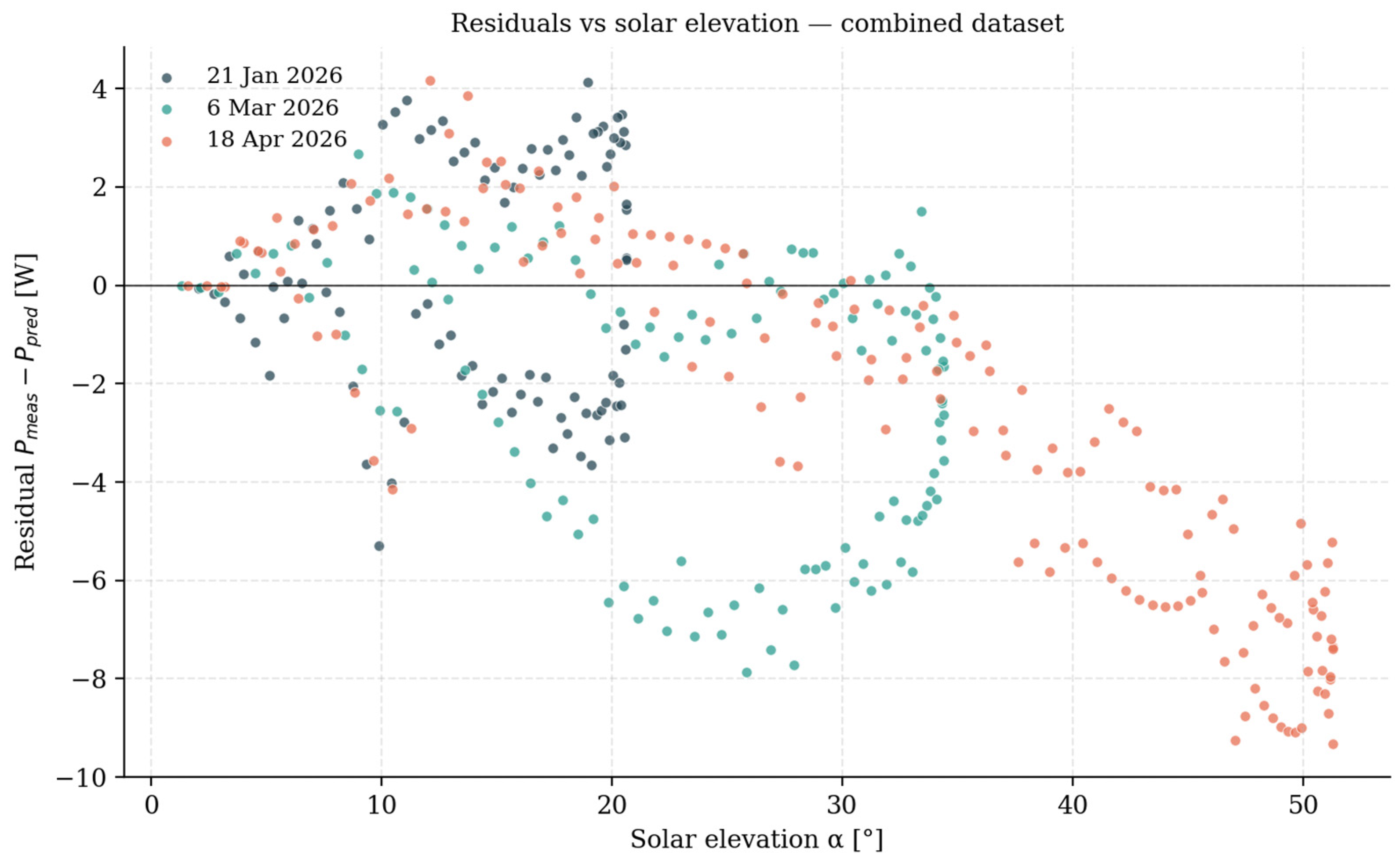
3]. At the low altitude of the validation campaign, the clear-sky diffuse component is no longer negligible, but its omission is bounded directly by the validation: because the ground measurements capture the total collected power, any missing diffuse contribution is already contained within the reported 6.0% RMS error. Consistent with this, the residuals at low solar elevation in results section—where the diffuse fraction is largest—are only slightly positive, at the level of under three watts, placing an empirical upper bound on the omitted term and indicating that it is partly offset by the temperature-driven over-prediction at high elevation. Second, the atmosphere is treated as a single broadband absorber characterised by one transmission coefficient, accurate to within a few percent for clear-sky conditions over the photovoltaic-relevant spectral band; spectral-resolved models exist [
36] but are not invoked here; the resulting broadband error is within the few-percent clear-sky envelope confirmed by the validation of
Section 4.4. Third, the pressure profile is the static U.S. Standard Atmosphere; real pressure departs from this mean by a few percent, a second-order effect on predicted irradiance that can be tightened with a measured profile if higher fidelity is required.
3.3. Wing-Geometry Solar Power Collection Model
The environmental irradiance model provides the direct-beam component on a horizontal reference surface. To translate this into the power actually collected by a solar array distributed over a curved, cambered wing with dihedral, an additional geometric model is required. Its objective is to reduce the wing geometry—airfoil shape, planform, dihedral, sweep and cell layout—to a small set of scalar coefficients that completely characterise its solar-collection behaviour at any sun position and aircraft heading. These coefficients enter the energy-balance computation as multipliers on the horizontal direct-beam irradiance, replacing the flat-plate assumption common in the solar-UAV sizing literature [
3,
7,
14].
3.3.1. Coordinate System and Surface Discretisation
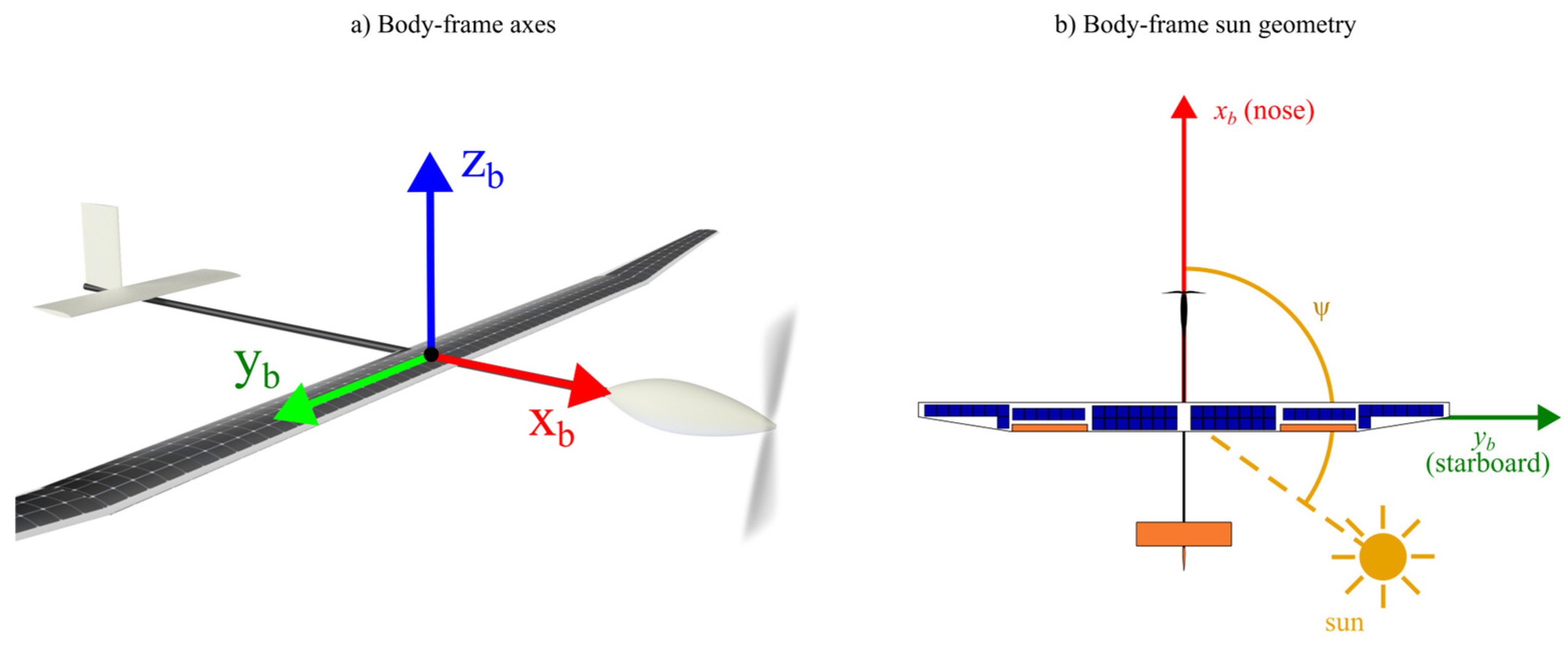
All quantities are expressed in an aircraft body frame (
Figure 3) with
x forward along the longitudinal axis,
y toward the starboard wing and
z vertically upward. The body-frame sun geometry is described by an azimuth
ψ, the clockwise angle from the nose to the sun in the horizontal plane and an elevation
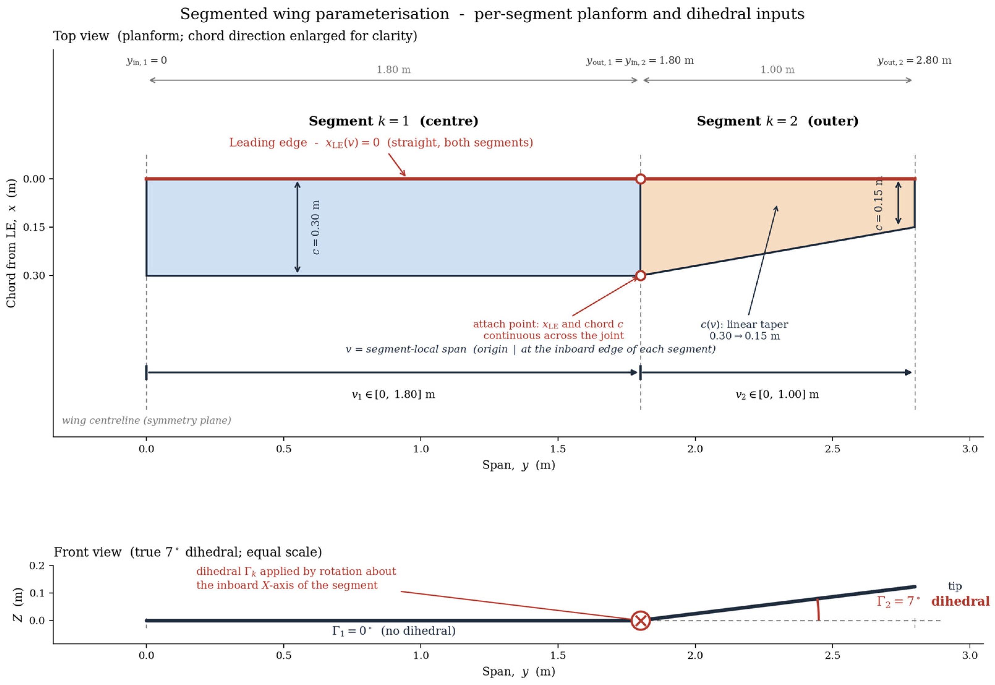
ε above the local horizon. The wing is composed of one or more spanwise segments, each defined by its inboard and outboard span positions, a dihedral angle and a planform table giving the leading-edge position and the local chord; the airfoil is supplied as a normalised upper-surface curve. Solar cells are defined as rectangular patches in the chord–span parameter space of the upper surface and are wrapped onto the three-dimensional wing geometry.
Each cell is divided into an
N ×
N grid of vertices, yielding (
N − 1)
2 quadrilateral surface elements. The default discretisation uses
N = 100, producing 9801 elements per cell; convergence tests confirm that further refinement changes the resulting coefficients by less than 10
−4. For each surface element, the area and outward unit normal are computed from the two diagonals
d1 and
d2 of the quadrilateral:
The sign of the normal is chosen so that all normals point outward from the upper surface. Summing across all cells and their mirrored counterparts for symmetric wings yields two quantities that fully characterise the discretised geometry—the area-weighted vector sum of element normals and the total active cell area:
Figure 4 shows the segmented-wing parameterisation, and
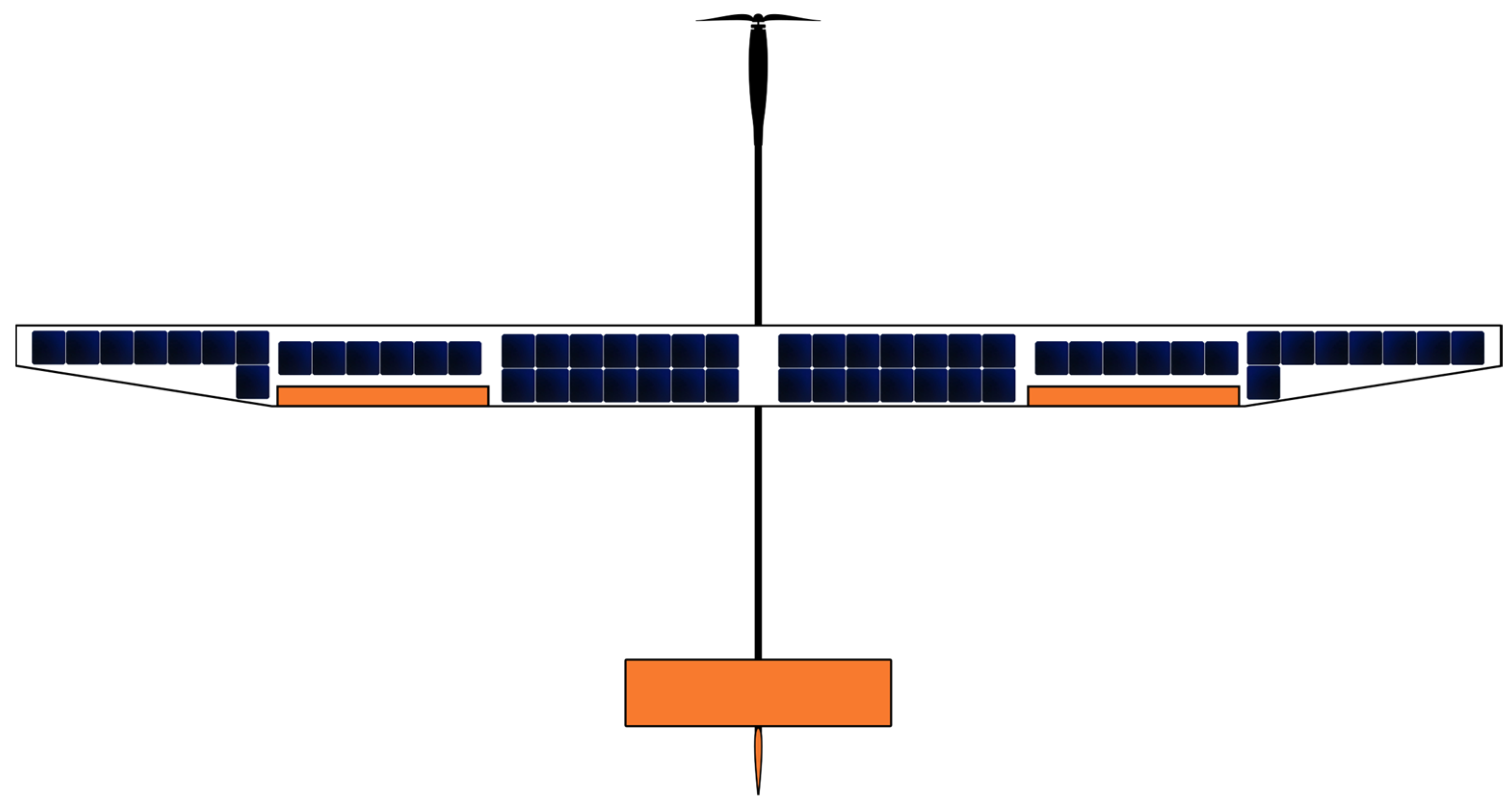
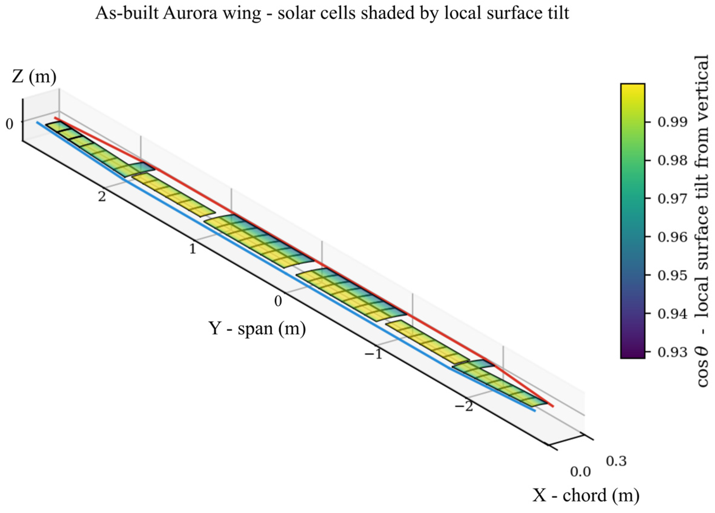
Figure 5 shows the as-built Aurora cell layout with elements coloured by local surface tilt, demonstrating that the computed normals capture the local orientation of the curved surface.
3.3.2. Direct-Beam Collection Coefficient
Let the unit vector pointing from the aircraft toward the sun be expressed in the body frame as
The direct-beam power received by an element is proportional to . A horizontal flat panel of the same total area receives .
The dimensionless collection coefficient
C is defined as the ratio of curved-wing collection to horizontal flat-panel collection:
For wings of realistic camber and modest dihedral operating at useful sun elevations, no upper-surface element turns its normal away from the sun, so the sum is taken over the full wing without clipping and becomes linear in the sun vector:
Explicitly, the area-weighted sum of element projections sT(∑ Ai ) is linear in the body-frame sun vector s, because each element contributes Ai (s · ) with no clipping. Collecting the three components of the area-weighted normal vector ∑ Ai and normalising by the total active area gives one scalar per body axis—the vertical component fixing the orientation-independent term and the two horizontal components fixing the heading-dependent pair (). The reduction to three scalars is therefore exact for the linearised (no-self-shading) regime, not an approximation.
This no-clipping condition concerns self-shadowing only: each element still contributes its own, individually oriented cosine projection, so the camber, dihedral and taper of the wing are fully retained in the coefficients and . It does not flatten the surface—a genuinely flat panel yields and .
Introducing three dimensionless coefficients that depend only on the wing geometry, formed from the components of the area-weighted normal,
the collection coefficient takes its final closed form:
Equation (19) is the central result of this subsection. The entire heading and elevation dependence of solar collection on a curved wing is captured by exactly three scalars—
—which are functions only of the wing geometry and cell layout. They are computed once per design iteration; the closed form is then evaluated analytically at run time for any (ψ, ε) pair, without further mesh integration. The amplitude of the heading-dependent variation and the heading at which collection peaks follow directly:
The heading-dependent term of Equation (19) is sinusoidal in
ψ with zero mean. For any trajectory whose heading uniformly traverses a full revolution—most notably a sustained circular loiter—the orbit-averaged collection coefficient reduces exactly to
This is an exact analytical result. It establishes that under closed circular flight, the curved-wing collection coefficient reduces, on average, to a constant scaling of the equivalent flat-panel collection, so heading dependence need not be carried through the diurnal energy-balance computation when the operating mode is continuous loitering. For mirror-symmetric wings, the lateral component vanishes () and the peak heading collapses to the sun being directly ahead or directly behind.
3.3.3. Conversion to Electrical Power
The collection coefficient is dimensionless. The electrical power produced by the wing-mounted array follows by scaling the horizontal flat-panel reference irradiance
IH by the total active cell area, the collection coefficient and the photovoltaic conversion efficiency:
where
is the photovoltaic conversion efficiency—the cell efficiency together with maximum-power-point tracking and the other electrical-path losses between array and bus. Equation (22) is the output of the solar prediction model: the quantity integrated over the diurnal cycle to evaluate the energy balance. Three assumptions bound the formulation. The no-self-shading condition is satisfied for moderate camber and dihedral below about 10° at solar elevations above roughly 5°, below which the closed form is slightly conservative and is not applied; the model treats the direct-beam component only, consistent with the irradiance model; and the geometric integrals are evaluated on the undeformed wing, with in-flight aeroelastic deformation a second-order effect [
37,
38].
3.4. Total Energy Balance Calculation
To evaluate the energy sustainability of a solar-powered UAV, the real-time energy consumption and solar generation are tracked over the whole mission, allowing the battery SoC to be computed at each step. The simulation begins with a fully charged battery and proceeds in discrete steps of duration
. During each step, the battery is charged by the solar energy generated and discharged by the constant onboard consumption
, the combined draw of propulsion, control, communication and payload systems:
The battery state of charge is then updated by the net energy gain or loss, with the result clipped between zero and the usable capacity B:
and, for a more practical interpretation, expressed as a percentage of full capacity:
The state of charge is modelled as a scalar energy reservoir in watt-hours. This high-level abstraction is widely used in early-stage system design, where modelling energy flows in terms of power and capacity is sufficient for feasibility studies and initial sizing. More detailed electrochemical models—capturing voltage dynamics, internal resistance and temperature dependence—exist, but that fidelity is not required here, where the objective is the system-level interaction between solar input, storage and consumption. Charge and discharge inefficiencies are represented by a single discharge-chain efficiency rather than an explicit electrochemical loss model. To maintain operational safety and prevent deep-discharge damage, a 30% minimum-SoC threshold is imposed as the operational reserve, reflecting standard practice in UAV battery management and the deep-discharge safety characteristics of lithium-ion cells [
17,
39]. Forward-Euler integration is used for the SoC dynamics; at the chosen time step, the truncation error is below the rounding noise of the battery model.
3.5. Software Architecture and Implementation
The framework is implemented as a modular, reproducible Python 3.13 toolchain divided into two cooperating modules. The irradiance module implements the solar-position and atmospheric relations of
Section 3.2 directly from the astronomical formulae, with no external solar-position library, so that the computation is fully auditable. The wing-geometry module reads an airframe description—segment topology and dihedral, an airfoil tabulation, one planform table per segment and a cell-layout table—and returns the three scalar coefficients and the total active area; these are computed once per airframe and saved, so that at run time, the closed form of Equation (19) is evaluated in a handful of floating-point operations. Both modules depend only on standard numerical libraries.
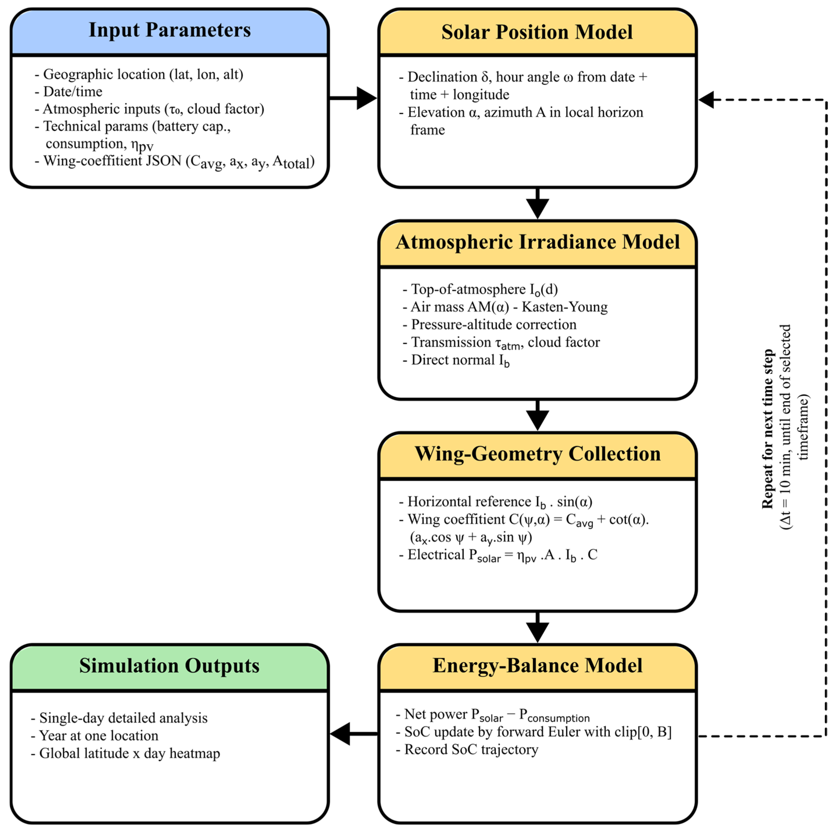
The temporal axis is discretised at a fixed interval, with a default of Δt = 10 min (144 samples per 24 h cycle), fine enough that further refinement changes the daily energy integral by less than 0.1%. Each iteration performs the four-stage evaluation chain—solar position, direct normal irradiance, wing-collected power and SoC update—and advances the time pointer. For annual and global modes, the simulation is integrated continuously across day boundaries, so the night-spanning portion of the SoC cycle is faithfully captured and the lowest SoC, which occurs at sunrise after a full night of consumption, is reported. The wing-geometry module includes two analytical verification configurations—a flat plate, for which the collection coefficient reduces exactly to unity, and a 10° dihedral plate with a known closed-form answer—both reproduced to five decimal places at the default grid resolution. All run-time parameters are exposed as named constants, so that re-running a script on a different machine reproduces the published figures exactly. The information flow within the combined model is shown in
Figure 6.
3.6. Analysis Modes
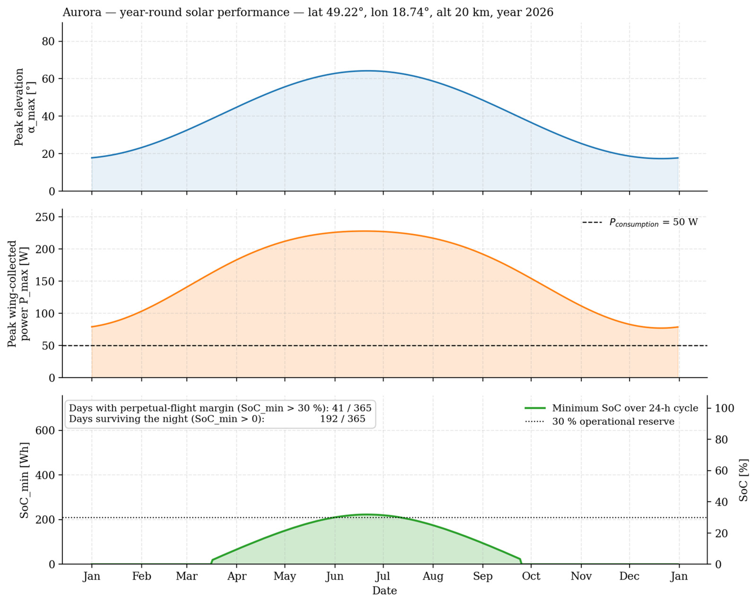
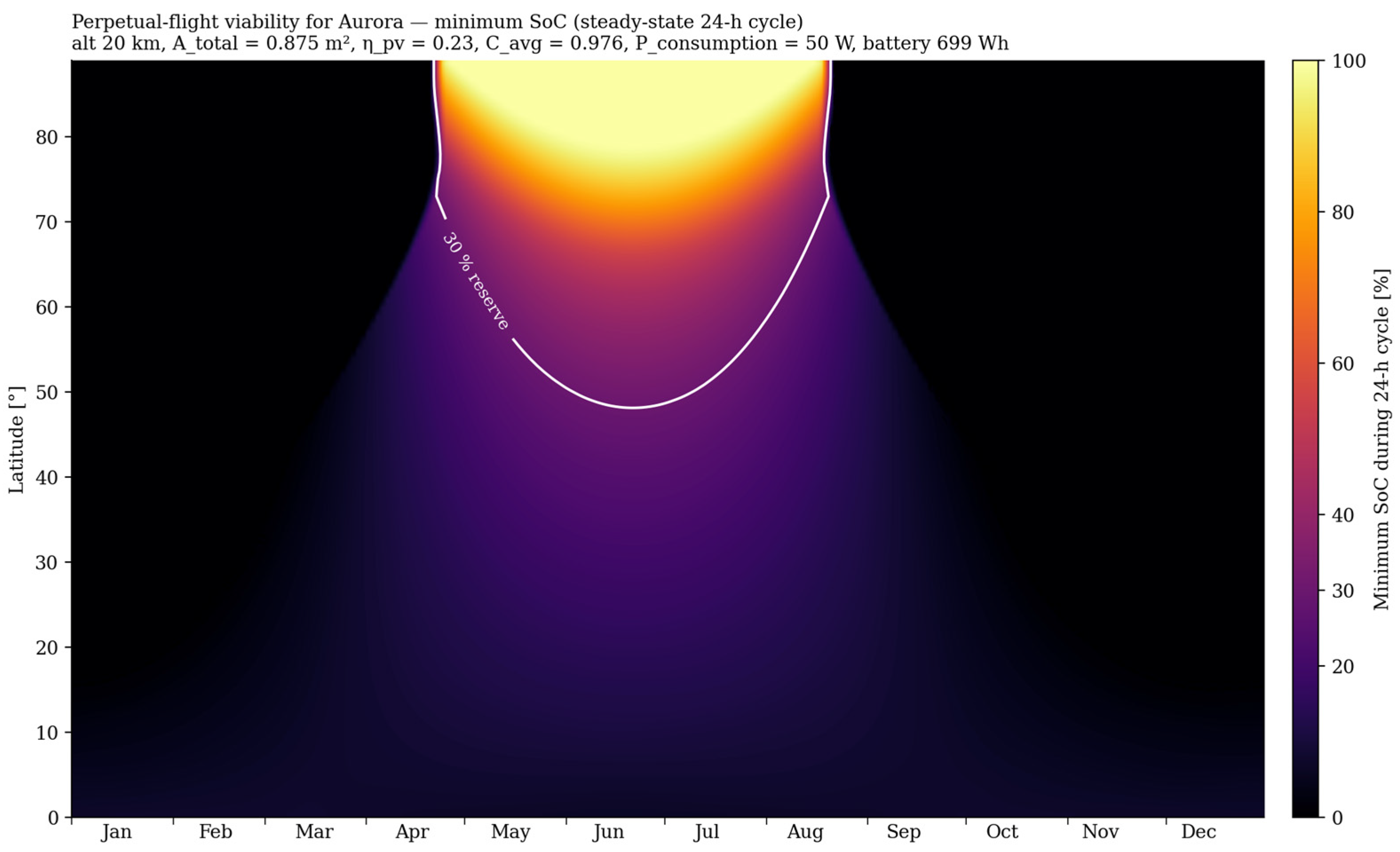
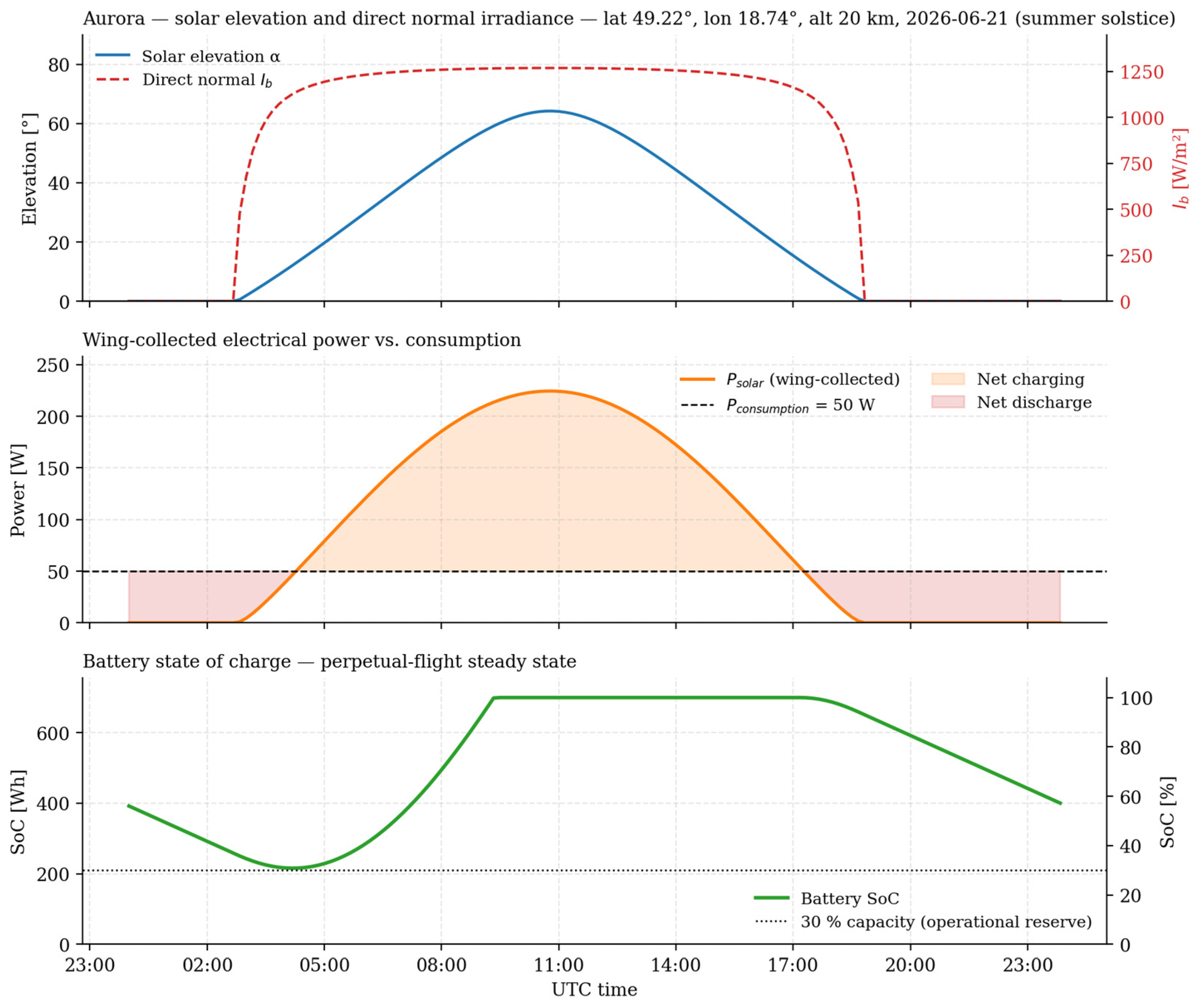
The combined model supports three analysis modes, which share the same underlying time-stepped physics and differ only in temporal and spatial scope and in the form of the summary product. Mode 1, single-day detailed analysis, evaluates one location, altitude and date at 10 min resolution across 24 h and produces three time-resolved trajectories—solar elevation and direct normal irradiance, wing-collected power against the consumption baseline and the SoC trajectory with the 30% reserve marked. Mode 2, year-at-location analysis, propagates the 10 min simulation continuously across all 365 days at one site and produces daily-aggregated traces together with two summary counts: the number of days on which the minimum SoC stays above the 30% reserve and the number of days on which the platform survives the night. Mode 3, global annual analysis, evaluates a latitude band across the full year and produces a two-dimensional heatmap of minimum SoC against latitude and day of year. A change to the underlying physics propagates automatically through all three modes by re-execution of the corresponding scripts.
3.7. Experimental Platform—Aurora
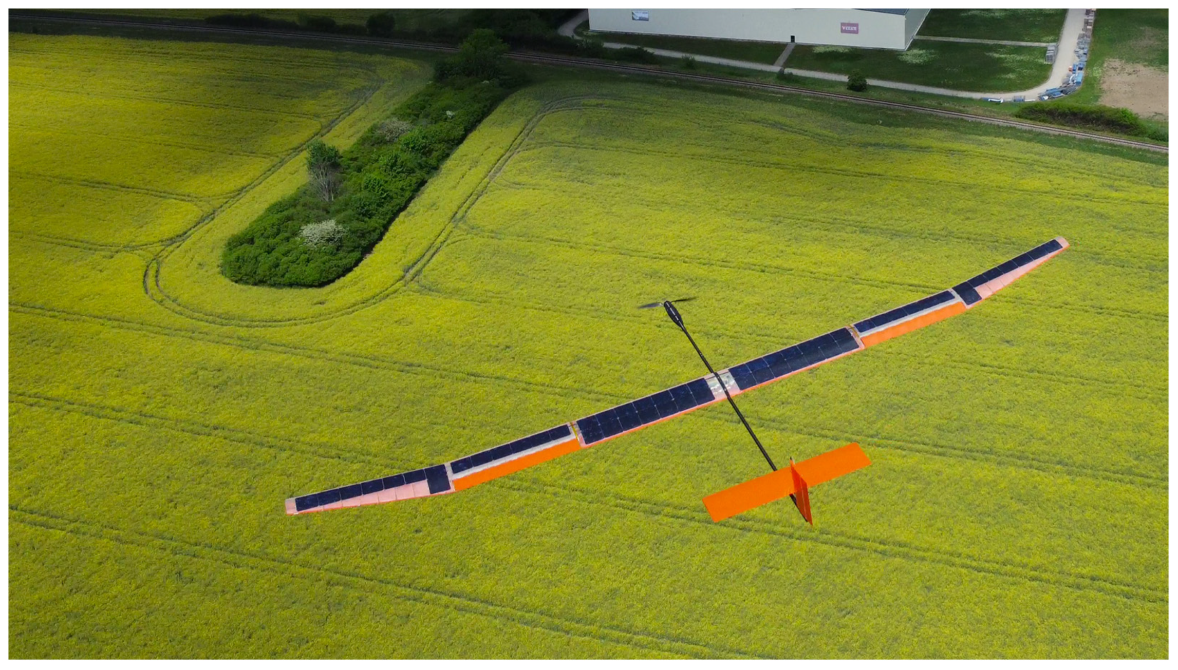
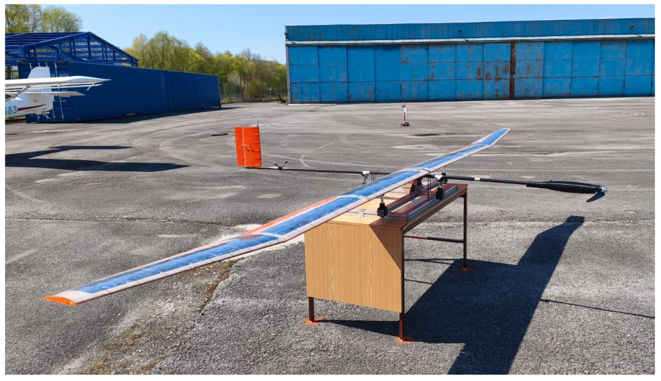
The framework is validated against measurements collected on Aurora, a solar-powered UAV demonstrator developed by the authors as a low-altitude precursor to a future stratospheric HAPS [
40] (
Figure 7 and
Figure 8). Aurora is a high-aspect-ratio solar motor-glider of conventional layout: a single tractor motor on the nose of a slender fuselage boom, a three-piece wing carried at mid-fuselage and a conventional tail with an all-moving horizontal stabiliser and a rudder. The principal dimensions are a wingspan of 5.6 m, an overall length of 2.95 m and a maximum take-off mass of approximately 8 kg. The wing divides spanwise into a 2.0 m untapered centre section at 0.30 m chord and two 1.8 m outer sections; each outer section carries an untapered inboard portion with the aileron, followed by a 1.0 m tapered panel that reduces the chord to 0.15 m at the tip and carries 7° of dihedral. The reference wing area is approximately 1.53 m
2, and the aspect ratio is approximately 20. The wing uses the Eppler E67 section throughout [
41], a low-Reynolds-number endurance airfoil whose polar was evaluated with a viscous–inviscid panel method [
42], and the primary structure is carbon-fibre, with a glass-laminate upper skin into which the solar cells are integrated.
The solar array comprises 56 SunPower C60 (Maxeon Solar Technologies, Singapore) monocrystalline-silicon cells (125 × 125 mm), 28 on the centre section and 14 on each outer section, for a total active cell area of 0.875 m
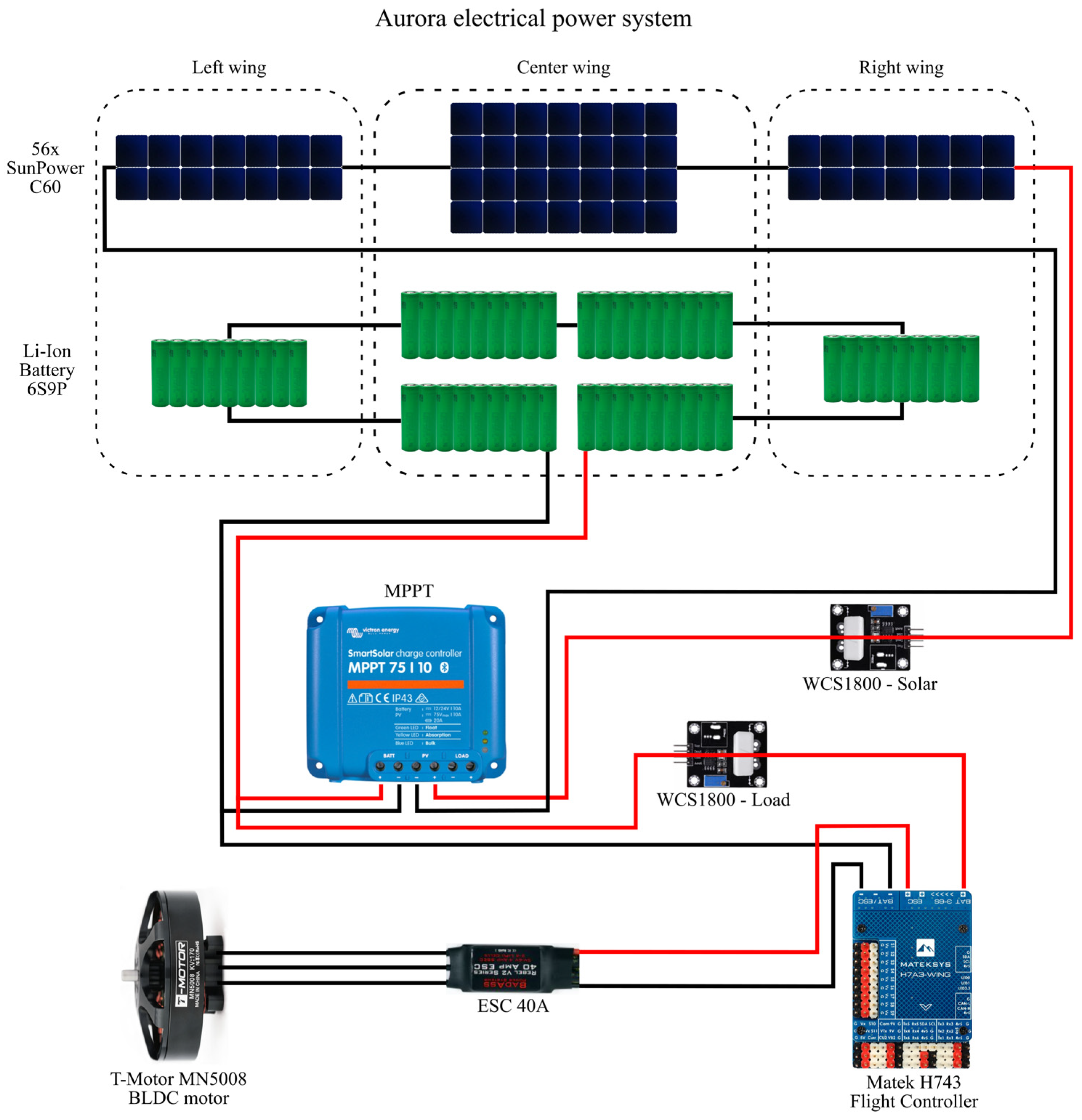
2. The cells are bonded directly to the upper glass-laminate skin with a compliant neutral-cure silicone adhesive, a deliberate choice that allows the high-aspect-ratio wing to flex in flight without transmitting bending strain into the brittle silicon, and are over-laminated with a clear protective film. Energy storage is a 6S9P lithium-ion pack of 54 high-capacity 18650 cells, giving approximately 699 Wh at a pack mass of about 2.91 kg (a pack-level specific energy of roughly 240 Wh kg
−1); the pack is physically distributed along the span for mass distribution. A Victron SmartSolar MPPT charge controller performs maximum-power-point tracking of the array. Propulsion is a single brushless DC motor with a 40 A speed controller driving an 18.5 × 15 inch propeller, selected with reference to established low-Reynolds-number propeller performance data [
43], and flight control is provided by an autopilot running the ArduPilot ArduPlane v4.6.2 firmware. The electrical power architecture is shown in
Figure 9.
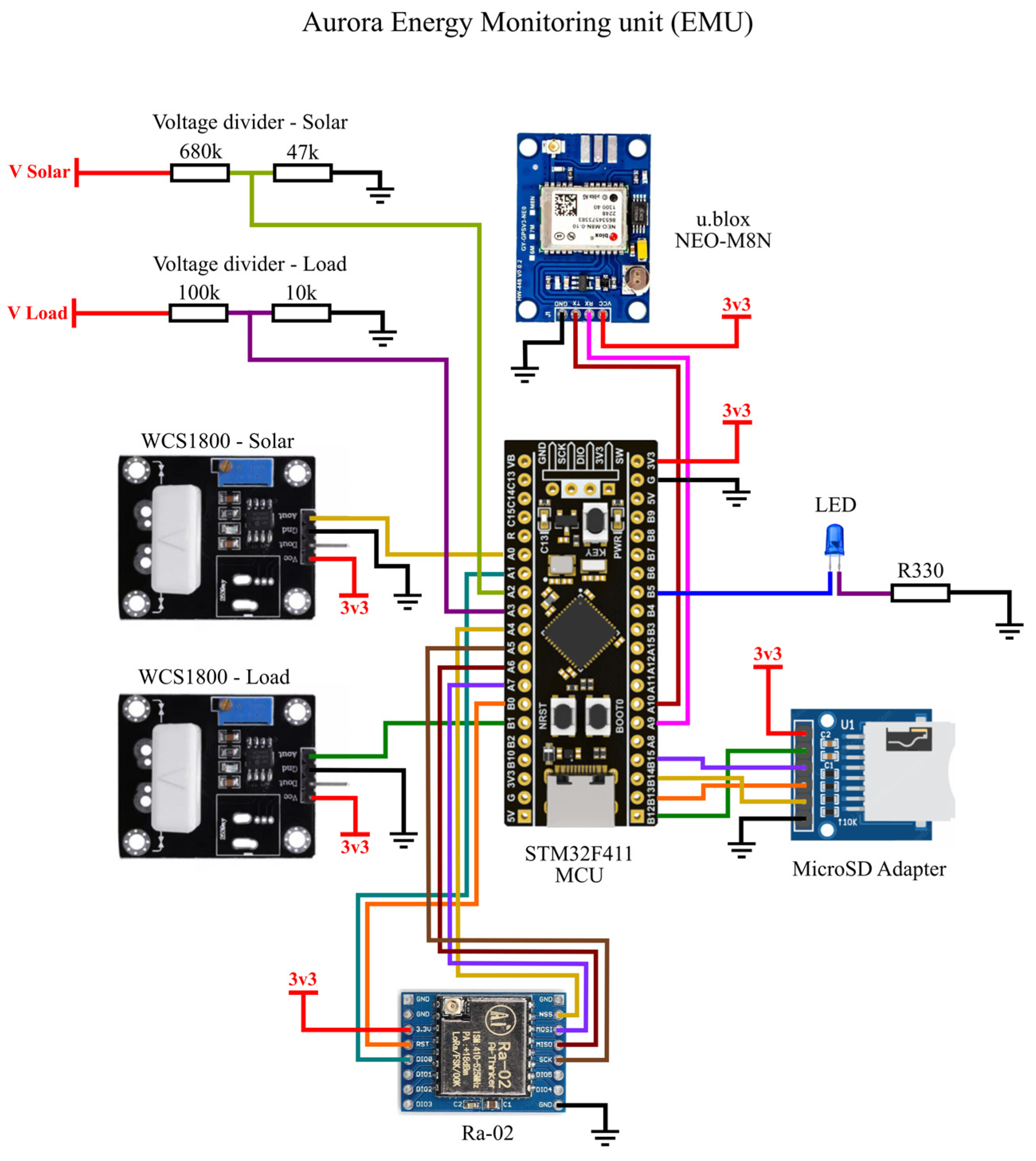
The measurements that validate the framework are collected by a purpose-built Energy Monitoring Unit (EMU), developed by the authors and shown schematically in
Figure 10. The EMU is built around an STM32 microcontroller; the solar and load currents are each measured by a Hall-effect current sensor and the corresponding voltages through resistive dividers, while position and time are provided by a GNSS receiver. The instrument logs the full-rate record to a microSD card and transmits a 1 Hz subset over a dedicated 433 MHz telemetry link—distinct from the aircraft’s command radio—to a custom ground station that overlays the live telemetry on the predicted solar-availability and SoC traces, allowing the modelled and measured energy budgets to be compared during operation.
5. Discussion
This study set out to develop and validate a simulation framework for the energy balance of solar-powered UAVs, with particular attention to the conversion from incident irradiance to collected electrical power. The results confirm that mission endurance—and especially the possibility of uninterrupted multi-day flight—is governed by the interaction of solar-irradiance availability, onboard power consumption and energy-storage capacity and that this interaction can be predicted with engineering accuracy by a lightweight, modular tool.
The principal methodological contribution is the wing-geometry collection model. By reducing an arbitrary cambered, dihedralled wing to only three scalar coefficients and a closed-form expression, the model removes the flat-plate assumption that pervades the solar-UAV sizing literature [
3,
7,
14] without imposing any run-time cost: the surface integration is performed once per airframe, and the diurnal energy balance then evaluates the closed form in a handful of operations. The flat-plate model that underlies prior frameworks corresponds exactly to C = 1 in the present formulation. For the Aurora array, the wing-geometry model returns an orbit-averaged C
0 = 0.976 and a heading amplitude set by C
1 = −0.183, so a flat-plate treatment would mis-state the orbit-averaged collected power by the C
0 offset and would discard the heading dependence entirely—precisely the terms the validation confirms. The improvement over the flat-plate baseline is thus quantified directly by the departure of the coefficients from unity, without a separate comparison campaign. The exact orbit-averaging result is practically significant—it shows that for the continuous-loiter operating mode of a HAPS, the heading dependence collapses to a single constant scaling of the flat-panel collection, so the heading need not be propagated through the design-loop energy balance, while remaining available as an explicit control variable for operational optimisation.
Although it is validated on a single airframe, the collection model is configuration-agnostic by construction: it ingests an arbitrary set of spanwise segments, planform tables, airfoils and cell patches, so fuselage-mounted cells, tapered or swept wings and multi-surface or multi-wing platforms are represented simply as additional surface patches in the same integration. The three-coefficient reduction and the closed form of Equation (19) hold for any such surface, provided the no-self-shading condition of
Section 3.3.3 is met; only the numerical values of C
0, C
1 and C
2 change with configuration.
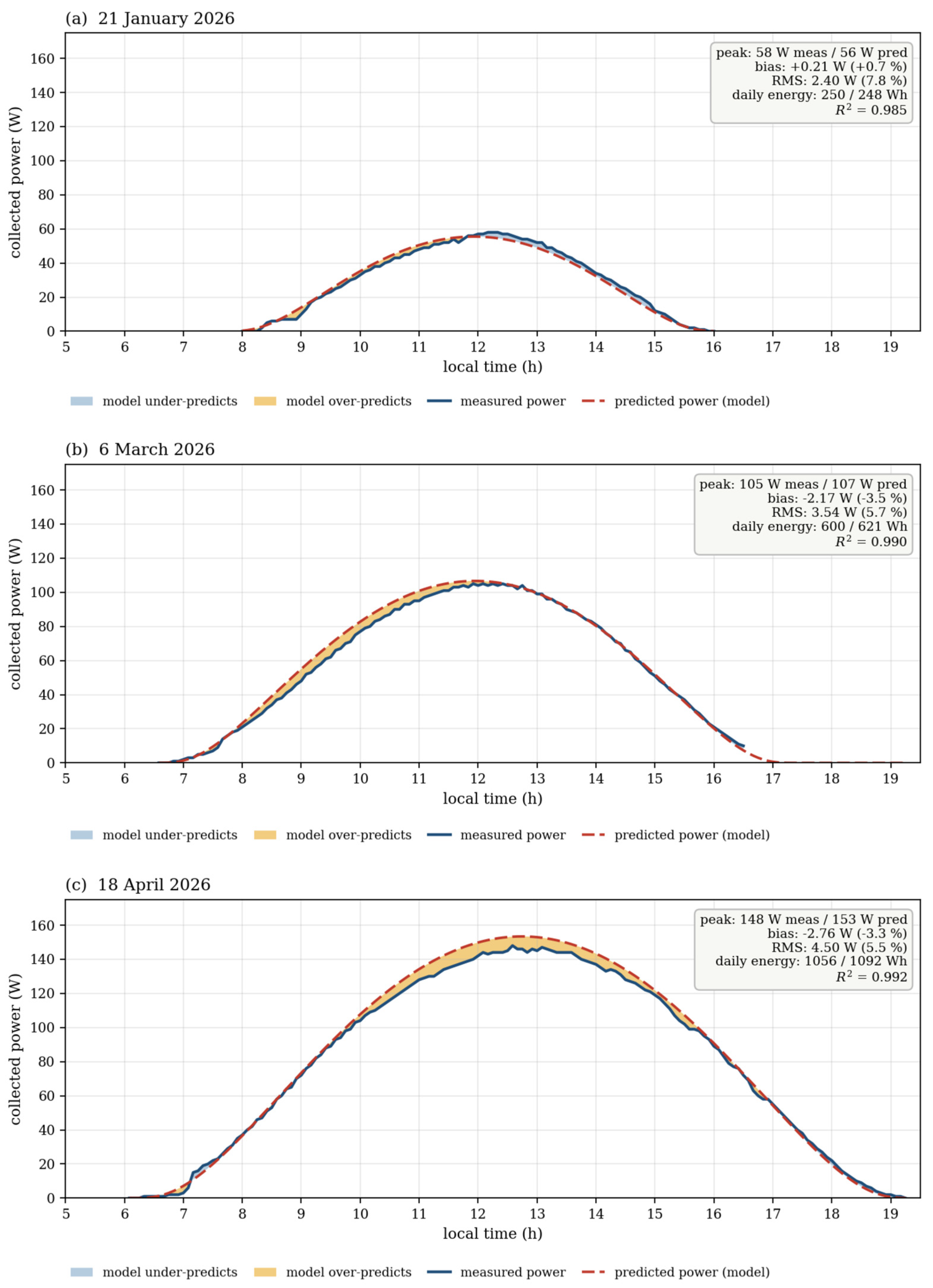
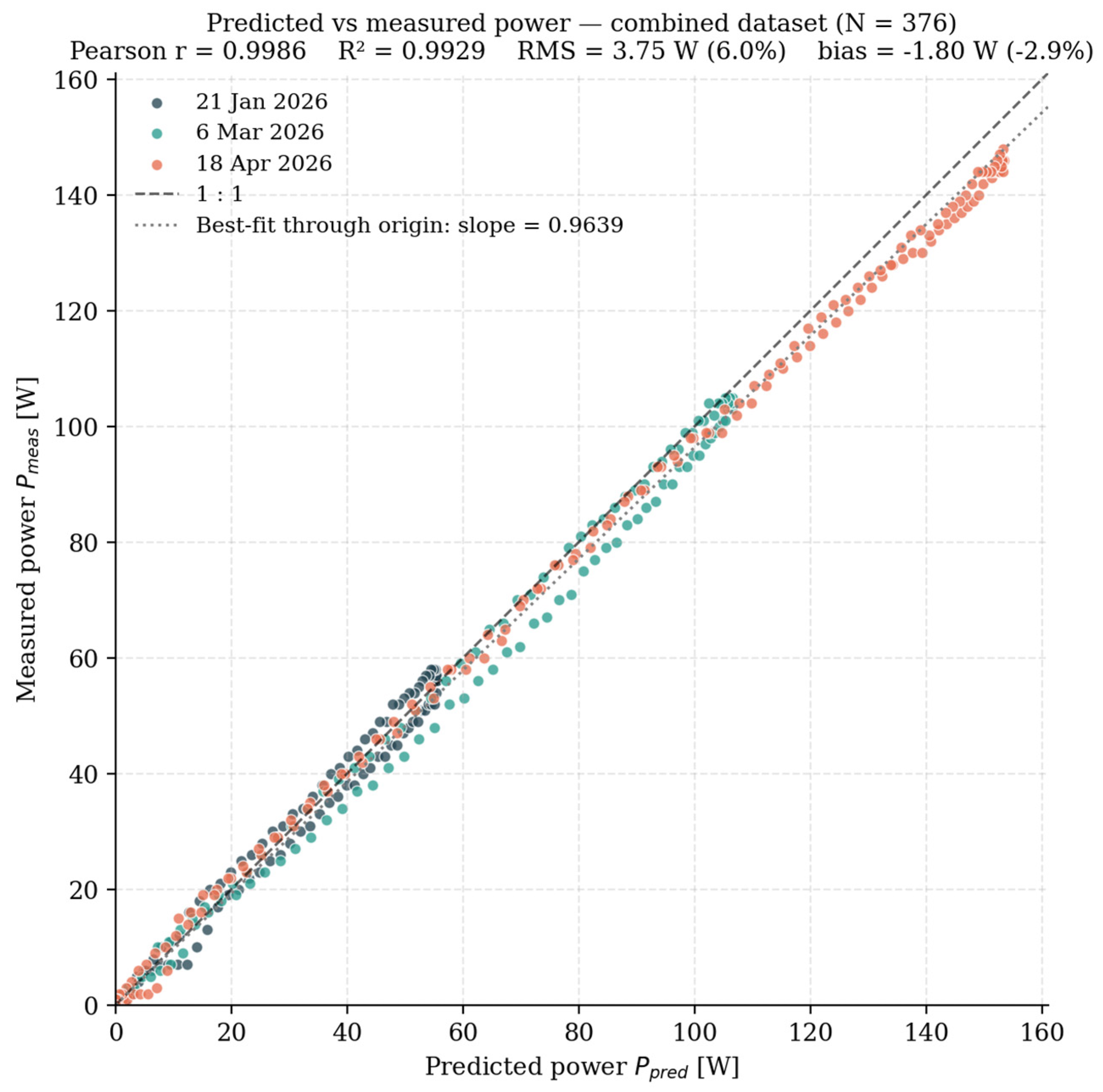
The validation against the Aurora charging campaign is the second contribution. Measurements taken on the real array of a real airframe gives the comparison direct relevance to the platform the framework is intended to support. The agreement is strong: across 376 samples spanning a 90-day seasonal range, the model reproduces the wing-collected power with a correlation of 0.998 and an RMS error of 6.0%, and—most importantly for design and planning use—the daily energy totals agree to within 3.5%. The structured residual is itself an informative result: rather than unexplained scatter, the disagreement has the clear elevation-dependent signature of photovoltaic temperature derating [
44], a known mechanism whose magnitude and trend match the observation and which can be added as a bounded, well-understood refinement.
A dedicated static heading-rotation campaign, indexing the airframe through controlled azimuths at fixed solar elevation, has separately been conducted on the Aurora platform and confirms the cos ψ heading dependence predicted by the collection model, with the pure-geometry coefficient found to be a conservative estimate of the realisable heading sensitivity. The detailed heading-resolved characterisation, together with the heading-optimisation strategy it supports, lies beyond the scope of the present energy-balance paper.
Several limitations should be stated. The validation was a ground-based campaign: the airframe was static, so the comparison does not exercise the thermal or aerodynamic conditions of flight, and although the test deliberately isolates the solar power-generation sub-model under natural sunlight, in-flight measurement campaigns will be needed to assess predictive accuracy in operational contexts. Four flight-specific effects warrant comment. First, because the collection model is formulated in the body frame for an arbitrary sun vector (Equation (19)), aircraft attitude enters the framework directly and can be driven by logged orientation; the static rig fixes attitude only to isolate the generation sub-model. Second, loiter bank angle perturbs the wing normal in a near-zero-mean fashion over a full circular orbit, so the orbit-averaged coefficient C
0 is essentially preserved, while cruise pitch is a small second-order change in effective elevation. Third, in-flight convective cooling lowers the cell-junction temperature relative to the static rig, which would reduce—not amplify—the high-elevation over-prediction identified in
Figure 17; the ground test is therefore a thermally conservative bound. Fourth, aeroelastic up-bending raises the effective dihedral in flight; this is a second-order effect on the geometric coefficients [
37,
38] and can be quantified directly, if required, by re-evaluating the wing-geometry module on the deflected wing shape.
The use of three clear-sky days is deliberate rather than a sampling limitation: the objective is to validate the deterministic clear-sky generation physics, for which clear-sky conditions are the correct controlled case that isolates the model from stochastic cloud effects. The three days span a 90-day seasonal range and a peak-elevation range of 20.6–51.3°, exercising the model across the geometric regime it is built to predict. Characterising performance under variable cloud is a separate task addressed by the configurable cloud-attenuation input and is not a validation of the clear-sky physics.
The irradiance model treats only the direct beam and uses a single broadband transmission constant and a static standard-atmosphere pressure profile; each of these is a small and, where relevant, conservative simplification, but each is also a natural target for higher-fidelity extension. The collection model assumes no self-shading and a rigid wing, both valid for the moderate camber and dihedral of the platforms of interest and at useful solar elevations. The onboard consumption is held constant at the cruise-mean value; because the energy balance is linear in consumption, a fractional change in mean power scales the overnight energy deficit proportionally, while transient wind- and gust-driven excursions largely average out over the diurnal integration. This assumption affects only the illustrative simulations of
Section 4.1,
Section 4.2 and
Section 4.3 and not the validation of
Section 4.4, in which the motor was cycled solely to keep the MPPT loaded. The battery is modelled as a scalar energy reservoir with a single discharge-chain efficiency; this is appropriate for feasibility screening and early sizing but not for precise mission-duration forecasting, for which an electrochemical model would be required.
From a broader perspective, the global analysis extends the applicability of the tool beyond a single mission. The finding that equatorial regions, despite receiving more direct sunlight, can face tighter endurance constraints than mid-latitude summers highlights that optimal deployment depends on the day–night energy balance and the duration of usable sunlight rather than on absolute irradiance alone and underscores the need for tailored design even in nominally favourable solar environments. Future work should incorporate an explicit photovoltaic temperature term, empirical cloud-attenuation data for tropospheric operation, dynamic rather than constant power consumption and integration with reanalysis or satellite-based irradiance datasets. The framework is also a natural foundation for energy-aware operational optimisation—heading and trajectory control, altitude profiling and model-predictive energy management—and for evolutionary or reinforcement-learning approaches to configuration tuning [
46,
47]. The closed-form, heading-resolved collection model is particularly well suited to such guidance applications, because it provides the heading–power relationship analytically and at negligible computational cost.
6. Conclusions
This paper presented a general-purpose, modular simulation framework for evaluating the energy balance and endurance potential of solar-powered UAVs. The framework couples a physics-based environmental irradiance model—astronomical solar position, air-mass- and altitude-scaled broadband atmospheric transmission and an eccentricity-corrected extraterrestrial reference—with a wing-geometry photovoltaic collection model that reduces an arbitrary cambered wing to three scalar coefficients and yields a closed-form, heading-resolved expression for collected power, together with an exact orbit-averaging result for circular loiter. Implemented as a reproducible tool with single-day, annual and global analysis modes, it enables rapid exploration of flight viability across configurations, latitudes and seasons.
The solar power-generation model was validated against a ground-based charging campaign on the as-built Aurora demonstrator over three clear-sky days spanning a 90-day seasonal range, achieving a predicted-versus-measured correlation of 0.998, a coefficient of determination of 0.993, an RMS error of 6.0% and a daily-energy agreement within 3.5%. A structured residual identified an unmodelled photovoltaic temperature effect, bounded at the 6% level and recommended as a future refinement. The framework provides HAPS designers and operators with a transparent, validated tool for feasibility screening, component selection and mission planning and offers a sound basis for the future integration of adaptive control strategies and real-time environmental feedback.