Trajectory Planning Framework for Drones Under Sensor Occlusion in Unknown Indoor Environments

Highlights

What are the main findings?

• A sensor occlusion detection algorithm is proposed for autonomous drone navigation in unknown indoor environments, which systematically classifies sensor occlusion into three categories: occlusion-free, partial occlusion, and full occlusion.
• An occlusion-aware trajectory replanning algorithm is proposed to handle partial and full occlusion conditions, generating candidate trajectories within occluded unknown regions to prevent collisions with obstacles.

What are the implications of the main finding?

• A novel trajectory planning framework is proposed for sensor occlusion scenarios, enhancing both the flight safety and navigation efficiency of drones operating autonomously in unknown indoor environments.
• The proposed framework can operate as an augmentation module while preserving the favorable characteristics of the underlying initial planning method, requiring only a 3D occupancy grid map and a parameterized trajectory.

Abstract

Autonomous drone navigation relies on onboard sensors to perceive obstacle information in real time. However, indoor environments contain abundant wall structures that occlude the sensor’s field of view, rendering obstacle information within occluded regions undetectable to the drone. Existing trajectory planning algorithms fail to adequately account for the safety risks introduced by sensor occlusion. To address this limitation, this article proposes a novel trajectory planning framework to enhance drone flight performance in indoor environments. Specifically, a 3D occupancy grid map is first constructed from sensor data, and an initial trajectory is generated from the current position to the goal. A sensor occlusion detection algorithm then classifies the current scene into three categories: occlusion-free, partial occlusion, and full occlusion. For occlusion-free scenarios, the initial trajectory is directly forwarded to the controller. For partial and full occlusion cases, an occlusion-aware trajectory replanning algorithm generates multiple candidate trajectories in unknown regions. These candidates are evaluated by a scoring function comprising three metrics: safety, efficiency, and smoothness. Upon detection of a collision between the currently executing initial trajectory and an obstacle, the active trajectory is immediately switched to the highest-scoring candidate trajectory, thereby ensuring both flight safety and navigation efficiency of the drone. Extensive experiments are conducted across multiple occlusion scene configurations to validate the performance of the proposed method. Experimental results demonstrate that the proposed method is capable of providing safe and efficient trajectories for drones under both partial occlusion and full occlusion conditions.

1. Introduction

In recent years, small-scale drones have attracted considerable research attention owing to their exceptional maneuverability [1,2,3], finding widespread applications across diverse domains, including agriculture and military operations [4,5,6]. When performing autonomous flight in unknown environments, drones rely on onboard sensors, such as depth cameras, to perceive surrounding environmental information and generate collision-free flight trajectories [7,8]. In indoor environments, however, surrounding walls introduce occlusions that compress the sensor’s perceptual space. Under such sensor-limited conditions, both the efficiency and safety of drone trajectory planning are severely compromised.

To date, no systematic classification of sensor occlusion levels caused by obstacles in indoor environments has been established. This article categorizes sensor occlusion into three classes based on the associated safety risk to the drone: occlusion-free, partial occlusion, and full occlusion:

• The occlusion-free case refers to scenarios in which no obstacles are present between the drone’s current position and the goal point within the sensor’s field of view, representing a condition with no associated safety risk.
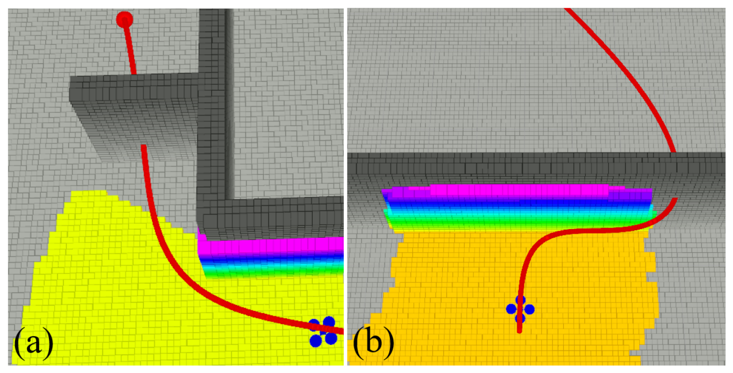
• The partial occlusion case, illustrated in Figure 1a, refers to the scenario in which obstacles partially obstruct the sensor’s field of view, creating blind spots within the effective sensing range. When obstacles are present within such unknown occluded regions, the risk of collision is substantially elevated.
• The full occlusion case, illustrated in Figure 1b, refers to the scenario in which an obstacle is sufficiently large to cause full occlusion of all feasible paths toward the goal within the sensor’s field of view. In this case, the drones face not only an increased collision risk but also the potential to become trapped in a local optimum replanning cycle, as no feasible trajectory toward the goal can be identified in the vicinity of the current position.

Figure 1. Illustration of (a) partial occlusion and (b) full occlusion conditions. These scenarios are commonly encountered in indoor environments, such as navigating corridor turns and bypassing wall obstacles.

Figure 1. Illustration of (a) partial occlusion and (b) full occlusion conditions. These scenarios are commonly encountered in indoor environments, such as navigating corridor turns and bypassing wall obstacles.

Existing planning strategies for sensor occlusion conditions can be broadly divided into two categories. The first is the conservative planning strategy [9,10], which constrains trajectory generation within the known map or the sensor’s field of view, treating unknown occluded regions as obstacle-occupied areas. While this approach maximizes flight safety, it inherently sacrifices trajectory flexibility and traversal efficiency. The second is the optimistic planning strategy [11,12,13], which treats unknown occluded regions as obstacle-free areas, allowing the planner to generate more aggressive trajectories. Although this approach improves both flexibility and efficiency, trajectories that penetrate unknown regions introduce non-negligible safety risks. To address the safety risks inherent in optimistic planning, the prevailing solution in the literature is the perception-aware planning approach [14,15]. The core principle of this paradigm is to incorporate visibility as an optimization objective, enabling the drones to observe unknown occluded regions earlier prior to entering them. This approach can effectively mitigate the risk of collision with obstacles in occluded regions for the partial occlusion case. However, to maximize visibility into occluded regions, perception-aware methods tend to deflect the trajectory away from the occluding obstacle, which comes at the cost of traversal efficiency. Furthermore, in full occlusion scenarios, such methods still fail to generate feasible and effective trajectories. When the occluding obstacle is sufficiently large, some improvements in visibility are still insufficient to expose the obstacle boundary, and therefore cannot break the local optimum in which the planner becomes trapped.

To overcome the limitations of existing approaches, this article proposes a novel drone trajectory planning framework tailored for indoor sensor-occlusion scenarios. A 3D occupancy grid map is first constructed from sensor data, upon which an initial trajectory is planned based on the observed obstacle information. When a segment of the initial trajectory is detected to pass through unknown regions, a sensor occlusion detection algorithm is invoked to classify the current scene into one of three categories: occlusion-free, partial occlusion, or full occlusion. For occlusion-free scenarios, execution of the initial trajectory proceeds without modification. For partial occlusion scenarios, an occlusion-aware trajectory replanning algorithm is triggered, comprising three stages: candidate trajectory generation, evaluation, and execution. In the generation stage, candidate trajectories are produced within unknown regions through a perception-range-based sampling strategy; in the evaluation stage, each candidate trajectory is scored by an evaluation function incorporating safety, efficiency, and smoothness criteria; and in the execution stage, a switching decision is made based on the collision status of the initial trajectory to determine whether it should be replaced by the highest-scored candidate. For full occlusion scenarios, an exploration vector is additionally integrated into the above pipeline to locate the obstacle boundary, thereby guiding the planner to generate a safe and efficient trajectory toward the goal.

The main contributions of this work are summarized as follows:

• A sensor occlusion detection algorithm is proposed to classify indoor sensor occlusion conditions into three categories: occlusion-free, partial occlusion, and full occlusion.
• An occlusion-aware trajectory replanning algorithm is proposed to handle partial and full occlusion scenarios, enhancing both trajectory safety and navigation efficiency.
• Comprehensive experiments are conducted in both simulated and real-world environments to validate the effectiveness of the proposed framework.

The remainder of this paper is organized as follows: related work on drone trajectory planning under occlusion conditions is presented in Section 2. A detailed description of the proposed algorithm is provided in Section 3, including the initial trajectory planning algorithm in Section 3.1; the occlusion detection algorithm in Section 3.2; and the occlusion-aware trajectory replanning algorithm in Section 3.3, which comprises the trajectory replanning algorithm for partial occlusion in Section 3.3.1 and the replanning algorithm for full occlusion in Section 3.3.2. Experiments and analysis are presented in Section 4, including simulation experiments for partial occlusion in Section 4.1, simulation experiments for full occlusion in Section 4.2, and real-world experiments in Section 4.3. Section 5 contains a discussion of the proposed method in Section 5.1 and a conclusion of the entire paper in Section 5.2.

2. Related Work

Considerable research effort has been devoted to drone trajectory planning in unknown environments. Fast-Planner [16] employs the distance field of an Euclidean Signed Distance Field (ESDF) map as a safety constraint, solving for collision-free, dynamically feasible, and smooth drone trajectories through B-spline trajectory optimization combined with gradient descent. To mitigate the high computational cost associated with ESDF construction, EGO-Planner [17] provides an ESDF-free gradient-based planning framework that generates collision-free trajectories via repulsive direction vectors. To address trajectory time minimization, Teissing et al. [18] introduce a time-optimal point-mass model and a limited thrust decomposition method to enable agile drone flight. The method in [19] guides the planner to generate reliable trajectories by monitoring structural changes in the local Euclidean Signed Distance Field, thereby enhancing trajectory safety and reducing the frequency of replanning. The problem of dynamic obstacle avoidance has been investigated in [20,21]. PE-Planner [20] integrates the planning framework of Fast-Planner with a local MPCC-based controller incorporating disturbance estimation and Control Barrier Function constraints, enabling high-speed flight in cluttered and dynamic environments. Qi et al. [21] propose a temporally constrained deep deterministic policy gradient reinforcement learning framework to address path planning in dynamic environments. The method [22] combines elastic visibility-aware trajectory planning with a flexible terminal adjustment algorithm to achieve adaptive dynamic tracking and perching for drones.

Regarding the safety risks posed by sensor occlusion conditions, Fast-Planner [16] provides only preliminary recognition of the potential flight hazards associated with trajectories passing in close proximity to obstacles, without dedicated optimization to address this concern. Faster [23] places greater emphasis on the collision risks introduced by obstacles lurking within occluded regions, and proposes the generation of backup trajectories within known-free regions as a means of enhancing flight safety. RAPTOR [15] introduces a perception-aware approach that quantifies safety risk through a trajectory visibility status and further optimizes the trajectory away from the occluding obstacle. This method enables the drone to observe unknown regions earlier during flight and has inspired a series of subsequent related works. For example, CPA-Planner [24] further extends the perception-aware planning framework of RAPTOR [15] by incorporating visibility as an explicit constraint during the path planning stage, thereby further enhancing the drone’s observational capability over occluded unknown regions. The study [25] introduces a viewpoint transition graph for adaptive target selection and a localizable corridor constructed via feature co-visibility evaluation, ensuring efficient navigation in unknown environments.

Although the aforementioned perception-aware methods can ensure trajectory safety under partial occlusion, they fail to deliver reliable performance in fully occluded scenarios. For instance, while the backup trajectory in FASTER guarantees flight safety, it does not retain any global information regarding obstacle boundary search; consequently, it cannot guide the drone toward the obstacle boundary under full occlusion. Similarly, perception-aware methods such as RAPTOR and CPA-Planner, even when trajectory visibility is maximized, remain unable to directly observe the obstacle boundary under full occlusion. As a result, both categories of methods are susceptible to local optima in fully occluded environments. In contrast, the proposed method introduces global obstacle-search information via an exploration vector, which effectively guides the drone to locate the obstacle boundary even under complete occlusion.

Several studies have also been devoted to addressing full occlusion caused by large obstacles [26,27]. For instance, the study [28] proposes a planning method for drones operating in unknown indoor environments based on a Limit Ellipsis Controller, which is an improved artificial-potential-field-type method capable of preventing the planner from becoming trapped in local optima. The method [29] employs hybrid surface frontiers to guide the trajectory search process, leveraging integrated information gain to improve trajectory feasibility. The study [30] addresses full occlusion of feasible paths induced by large obstacles through a cost-function-based backtracking and circumvention mechanism. Nevertheless, although the aforementioned methods can guarantee that the planner escapes local optima, they tend to explore redundant trajectories in the vicinity of the obstacle before identifying a feasible path toward the goal, failing to ensure energy-optimal trajectory generation. Meanwhile, frontier-based and backtracking-based methods also fail to guarantee the safety of occluded trajectory segments under partial occlusion. The proposed method, by contrast, not only leverages the exploration vector to rapidly identify the obstacle boundary under full occlusion but also employs candidate trajectories to ensure trajectory safety in partial occlusion scenarios.

3. Methodology

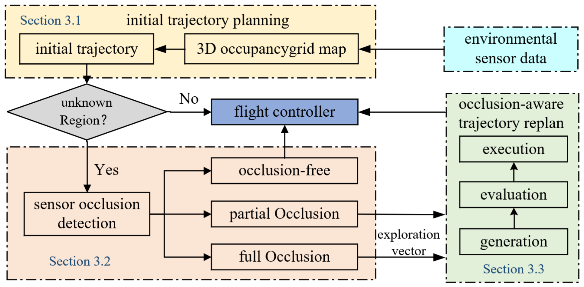
The overall pipeline of the proposed framework is illustrated in Figure 2. First, a 3D occupancy grid map is constructed from the surrounding sensor data, upon which an initial trajectory is planned (Section 3.1). The initial trajectory is then periodically inspected to determine whether any segment falls within unknown regions; if so, a sensor occlusion detection algorithm is applied to classify the current scene into one of three categories: occlusion-free, partial occlusion, or full occlusion (Section 3.2). For scenarios in which sensor occlusion is detected, an occlusion-aware trajectory replanning algorithm is invoked to ensure both the safety and efficiency of quadrotor flight (Section 3.3).

3.1. Initial Trajectory Planning

As demonstrated in [17], ESDF maps impose a heavy computational burden. Therefore, the proposed framework instead constructs a more fundamental yet computationally efficient 3D occupancy grid map from sensor data. Let the occupied, free, and unknown regions within the drone’s current grid map be denoted as ${\mathcal{X}}_{occ}$, ${\mathcal{X}}_{free}$ and ${\mathcal{X}}_{unk}$, respectively. The current drone position and local goal are denoted as ${\mathbf{p}}_{cur}\in {\mathbb{R}}^3$ and ${\mathbf{p}}_{goal}\in {\mathbb{R}}^3$. A collision-free path from ${\mathbf{p}}_{cur}$ to ${\mathbf{p}}_{goal}$ is then searched using the A-star algorithm. The resulting path is subsequently refined through B-spline curve optimization, improving both trajectory smoothness and dynamic feasibility. The optimization problem is formulated as follows:

$$\underset{\mathbf{C}}{min}\mathcal{J}={\lambda }_s{J}_s+{\lambda }_d{J}_d+{\lambda }_c{J}_c$$

(1)

where $\mathbf{C}=\{{\mathrm{C}}_0,{\mathrm{C}}_1,\dots ,{\mathrm{C}}_{N_c}\},{\mathrm{C}}_i\in {\mathbb{R}}^3$ denotes the set of control points for the drone trajectory, $J_s$ is the smoothness penalty, $J_d$ is the feasibility penalty, and $J_c$ is the obstacle collision penalty. $J_s$ is formulated as the time integral over square derivatives of the trajectory. $J_d$ is ensured by restricting the higher order derivatives of the trajectory on every single dimension. $J_c$ pushes control points away from obstacles. ${\lambda }_{*}\in \mathbb{R}$ are the weights that balance these penalty terms (detailed in [17]). The initial trajectory is denoted as $\mathcal{T}$. Since the primary focus of this work is on sensor occlusion detection and occlusion-aware trajectory replanning, the initial trajectory generation adopts straightforward path search and trajectory optimization algorithms. Notably, these components are modular and can be replaced by more advanced methods, such as [31,32], without affecting the subsequent stages of the framework. The proposed framework imposes only two requirements on the initial trajectory planning method: a 3D occupancy grid map and a parameterized trajectory, both of which are fundamental prerequisites in trajectory planning algorithms. Once these requirements are satisfied, the proposed framework can operate purely as an augmentation module when encountering occluded unknown regions while preserving the favorable characteristics of the underlying initial planning method.

3.2. Sensor Occlusion Detection

3.2.1. Algorithm Procedure

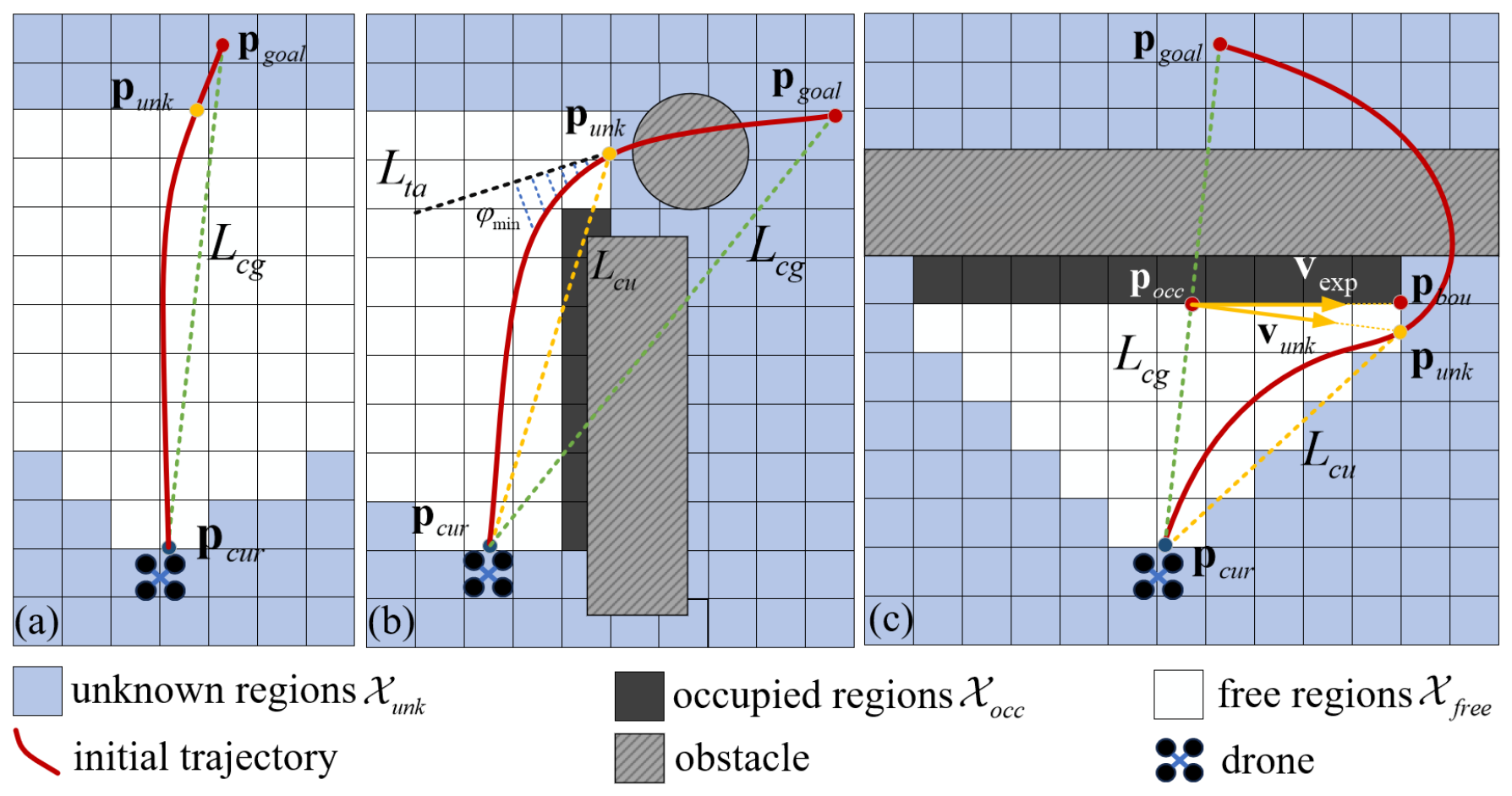
Let the occupied, free, and unknown regions within the drone’s current grid map be denoted as ${\mathcal{X}}_{occ}$, ${\mathcal{X}}_{free}$ and ${\mathcal{X}}_{unk}$, respectively. Upon generation of the initial trajectory $\mathcal{T}$, a periodic inspection is performed to determine whether any segment of $\mathcal{T}$ falls within the unknown region ${\mathcal{X}}_{unk}$. The first unknown point detected along $\mathcal{T}$ is denoted as ${\mathbf{p}}_{unk}\in {\mathbb{R}}^3$. The sensor occlusion detection algorithm is presented in Algorithm 1 and Figure 3. The algorithm first determines whether any obstacle exists between ${\mathbf{p}}_{cur}$ and the ${\mathbf{p}}_{goal}$ (Lines 2–4). If no obstacle is detected, the current scene is deemed free of collision risk and the algorithm returns the occlusion-free directly. Otherwise, the line segment $L_{cu}$ connecting ${\mathbf{p}}_{cur}$ and ${\mathbf{p}}_{unk}$ is constructed to facilitate further occlusion classification (Line 5).

The partial occlusion case typically arises when the trajectory undergoes a turning maneuver, causing obstacles to obstruct a portion of the sensor’s field of view, as shown in Figure 3b. When an occupied grid cell is detected on $L_{cu}$ (Line 6), it indicates that the unknown region at ${\mathbf{p}}_{unk}$ arises because the sensor’s view is blocked by a nearby obstacle. Furthermore, since ${\mathbf{p}}_{unk}$ is the first unknown point along the trajectory, a known region must necessarily exist in the vicinity of ${\mathbf{p}}_{unk}$, indicating that the sensor is able to detect the boundary of the occluding obstacle, which confirms that the obstacle causes only partial occlusion of the sensor. Once partial occlusion is determined, the severity of the current occlusion is assessed based on the average curvature of the trajectory as it approaches ${\mathbf{p}}_{unk}$. A larger curvature indicates that the occluded region is more difficult to discover. When the drone needs to turn sharply around the occluding obstacle in order to observe the occluded unknown region, the remaining planning margin becomes extremely limited, thereby increasing the risk of collision. Therefore, rather than relying on an ESDF map as required in [15], the threat level of the current scenario to flight safety is assessed by analyzing the local curvature of the trajectory. Specifically, the tangent line $L_{ta}$ to the trajectory at ${\mathbf{p}}_{unk}$ is first computed (Line 7). The time interval from $t_{unk}$ to $t_{cur}$ is then discretized into a decreasing sequence ${\mathcal{S}}_n=\{t_n,t_{n-1}\dots ,t_1\}$ with a uniform time step (Line 8). Starting from $t_{unk}$, the perpendicular distance $d_i$ from the trajectory position $\mathbf{p}\left(t_i\right)$ to the tangent line $L_{ta}$ is computed for each sampled time (Lines 9–10). If $d_i$ exceeds the minimum visibility distance ${\phi }_{min}$ and the mean curvature of the initial trajectory over the interval $[t_i,t_{unk}]$ surpasses the threshold $K_t\in \mathbb{R}$, the partial occlusion scenario is classified as posing a significant threat to flight safety (Lines 11–12).

Algorithm 1: sensor occlusion detection

Full occlusion typically occurs in scenarios where the drone needs to bypass a large wall-like obstacle. When an occupied grid cell is detected on $L_{cg}$, this indicates the presence of an obstacle between the drone and the goal point. If, at this moment, no occupied grid cell is detected on $L_{cu}$, it indicates that the current point $p_{unk}$ does not arise from obstacle occlusion. There are two possible causes for this phenomenon: first, a large obstacle may have fully occluded the sensor, such that no feasible obstacle-bypassing trajectory can be found within the current sensor range; second, a small obstacle may happen to lie exactly at the intersection of $L_{cg}$ and the edge of the sensor’s perception range. Let ${\mathbf{p}}_{occ}\in {\mathbb{R}}^3$ denote the intersection point between the line segment $L_{cg}$ and the obstacle (Line 15). The grid cells in the vicinity of ${\mathbf{p}}_{unk}$ are searched to identify the occupied cell closest to ${\mathbf{p}}_{unk}$, denoted as ${\mathbf{p}}_{bou}$, which represents the boundary point of the obstacle within the current sensing horizon (Line 16). The vector from ${\mathbf{p}}_{occ}$ to ${\mathbf{p}}_{bou}$ is defined as the exploration vector as ${\mathbf{v}}_{exp}\in {\mathbb{R}}^3$, and the vector from ${\mathbf{p}}_{occ}$ to ${\mathbf{p}}_{unk}$ is denoted as ${\mathbf{v}}_{unk}\in {\mathbb{R}}^3$ (Line 17). The following computation is then performed to determine whether a full occlusion condition is present (Lines 18–19):

$$1-{\displaystyle \frac{{\mathbf{v}}_{exp}·{\mathbf{v}}_{unk}}{∥{\mathbf{v}}_{exp}∥∥{\mathbf{v}}_{unk}∥}}<{\mathrm{C}}_t$$

(2)

$${\displaystyle \frac{∥{\mathbf{v}}_{\exp }∥}{∥{\mathbf{p}}_{occ}-{\mathbf{p}}_{cur}∥}}>R_t$$

(3)

where $C_t\in \mathbb{R}$ denotes the trajectory angle threshold and $R_t\in \mathbb{R}$ denotes the obstacle size threshold. When both Equations (2) and (3) are simultaneously satisfied, the obstacle is considered sufficiently large and the trajectory entering the unknown region is in close proximity to the obstacle, upon which the algorithm returns full occlusion (Line 18–19). Otherwise, the occlusion-free classification is returned (Line 21).

3.2.2. Threshold Determination

The sensor occlusion detection algorithm involves three detection thresholds, $K_t$, $C_t$, and $R_t$. The selection of these three thresholds has a substantial impact on the algorithm’s performance.

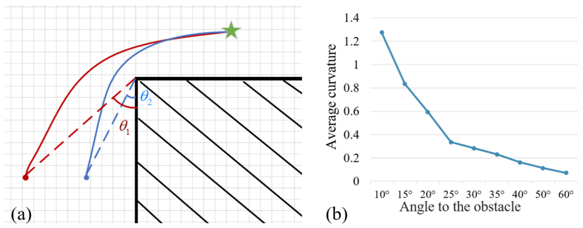
The selection of the threshold $K_t$ directly affects the algorithm’s sensitivity in classifying a scene as partial occlusion. If $K_t$ is set too small, scenarios with mild sensor occlusion may be misclassified as partial occlusion, triggering unnecessary replanning and resulting in computational overhead. Conversely, a larger $K_t$ significantly increases the probability of missing partial occlusion scenarios, thereby elevating safety risks during drone flight. In this paper, an appropriate value for $K_t$ is determined through empirical evaluation. As illustrated in Figure 4a, the experimental setup involves initiating multiple trajectory planning tasks from positions where the sensor faces the obstacle at varying angles ${\theta }_{*}$. For each configuration, the average curvature of the planned trajectory is computed. A smaller angle ${\theta }_{*}$ corresponds to more severe occlusion in the region behind the obstacle, which yields a larger average trajectory curvature. The statistical results are presented in Figure 4b. To balance safety and computational efficiency, $K_t$ is set to 0.25, which corresponds to an occlusion angle of approximately 30 degrees.

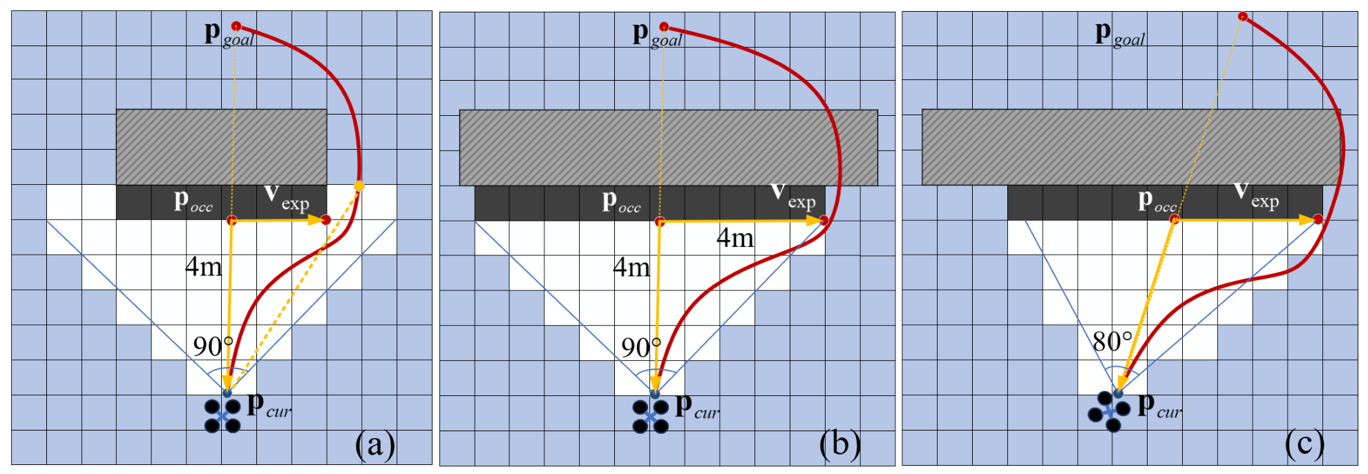
The obstacle size threshold $R_t$ is used to measure the size of an obstacle and is determined based on the sensor’s field of view and effective sensing range. For a commonly used camera such as the D435, the effective sensing range $d_s$ is approximately 4 m, with a horizontal field of view of approximately 90°. When an obstacle happens to be located precisely at the intersection of $L_{cg}$ and the edge of the sensor’s sensing range, no occupied grid cell will be detected on $L_{cg}$ either, as illustrated in the Figure 5a. In this case, the size of the obstacle directly in front of the drone can be approximately expressed as $d_s·R_t$. Under the ideal scenario of full occlusion, as illustrated in the Figure 5b, when the edge of the sensor is completely occupied by the obstacle, $R_t$ = 1. However, in practice, the drone’s viewing angle is unlikely to be perfectly aligned with the obstacle, and the data near the edge of the sensor’s field of view tends to become unreliable, effectively narrowing the usable field of view, which causes the value of $R_t$ to be smaller than 1, as illustrated in the Figure 5c. Therefore, a value of 0.5 is selected as the threshold $R_t$, meaning that an obstacle must be at least 4 m in size to exceed the threshold. This choice effectively filters out small obstacles that happen to appear at the intersection of $L_{cg}$ and the edge of the sensor’s sensing range while also avoiding missed detections of genuine full-occlusion scenarios due to an excessively large $R_t$ value. If a sensor with different parameters is adopted, the value of $R_t$ can be estimated by following the procedure described above.

For the trajectory angle threshold $C_t$ used in the full occlusion determination algorithm, it measures the cosine distance between ${\mathbf{v}}_{exp}$ and ${\mathbf{v}}_{unk}$. Under full occlusion, since the planner cannot find a known-free region between the obstacle and the target point, the trajectory is guided toward the unknown region near the obstacle, causing the distance between ${\mathbf{p}}_{unk}$ and ${\mathbf{p}}_{bou}$ to become very small. The threshold of $C_t$ can be estimated based on the obstacle inflation coefficient and the drone’s dimensions. For example, when the value of $C_t$ is set to 0.15, it means that the full occlusion condition is satisfied when the angle between ${\mathbf{v}}_{exp}$ and ${\mathbf{v}}_{unk}$ is smaller than approximately 30°. If $C_t$ is set too small, e.g., 0.05, the algorithm’s ability to detect full occlusion would be compromised, leading to missed detections. Conversely, if $C_t$ is set too large, the threshold would lose its discriminative effectiveness.

3.3. Occlusion-Aware Trajectory Replanning

3.3.1. Strategy for Partial Occlusion Conditions

In partial occlusion conditions, the worst-case configuration places an obstacle at the boundary between the known free region and the unknown region. By the time the drone detects the obstacle, the separation distance between them may already be critically small. If the motion planner is unable to generate a collision-free trajectory within the available reaction time, the drone faces the risk of abrupt deceleration or even collision. To this end, an occlusion-aware trajectory replanning algorithm is proposed to proactively generate candidate trajectories within the unknown region, ensuring flight safety while preserving trajectory flexibility.

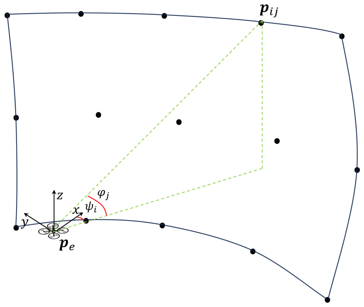
Generation: The perception-range-based sampling strategy for candidate trajectory generation involves four components: initial conditions, sampling region, terminal conditions, and parameterization. Let $t_c$ denote the timestamp at which the partial occlusion criterion is satisfied in the sensor occlusion detection algorithm (Algorithm 1 Line 11–12). The starting point of each candidate trajectory is located at the position on $\mathcal{T}$ corresponding to time $t_e=t_c+t_m$, where $t_m$ is a temporal relaxation factor. The position ${\mathbf{p}}_e\in {\mathbb{R}}^3$, velocity ${\mathbf{v}}_e\in {\mathbb{R}}^3$, and acceleration ${\mathbf{a}}_e\in {\mathbb{R}}^3$ of the initial trajectory at $t_e$ are recorded and used as the initial conditions for the candidate trajectories. Taking ${\mathbf{p}}_e$ as the starting point, the sampling region in the horizontal and vertical directions is defined as $[-{\theta }_h,{\theta }_h]$ and $[-{\theta }_v,{\theta }_v]$, respectively, based on the current sensor attitude and maximum sensing range. Sampling directions are then discretized along both the horizontal and vertical axes, enabling the candidate trajectories to uniformly cover the sensor’s perceptual space at ${\mathbf{p}}_e$, as illustrated in Figure 6. The terminal position of each candidate trajectory can be computed as follows:

$$\begin{array}{cc}\hfill {\mathbf{p}}_{ij}& ={\mathbf{p}}_e+(rcos{\phi }_{j}cos{\psi }_i,rcos{\phi }_{j}sin{\psi }_i,rsin{\phi }_j)\hfill \\ \hfill {\psi }_i& =-{\theta }_h+i\Delta {\sigma }_h,i=0,1,2,\cdots ,N_{\psi }\hfill \\ \hfill {\phi }_j& =-{\theta }_v+j\Delta {\sigma }_v,j=0,1,2,\cdots ,N_{\phi }\hfill \end{array}$$

(4)

where $\Delta {\sigma }_h$ and $\Delta {\sigma }_v$ denote the angular sampling intervals in the horizontal and vertical directions, and $N_{\psi }={\displaystyle \frac{2{\theta }_h}{\Delta {\sigma }_h}}$ and $N_{\phi }={\displaystyle \frac{2{\theta }_v}{\Delta {\sigma }_v}}$ represent the number of sampling points along the corresponding directions. r denotes the sampling length, computed according to the following formula:

$$r=min\left(r_{max},{\omega }_{\alpha }{\parallel {\mathbf{p}}_{goal}-{\mathbf{p}}_{unk}\parallel }^2\right)$$

(5)

where $r_{max}$ denotes the maximum length of the candidate trajectory and ${\omega }_{\alpha }$ is a scaling parameter. The terminal velocity ${\mathbf{v}}_{ij}\in {\mathbb{R}}^3$ of each candidate trajectory is decomposed into two components: speed magnitude and velocity direction. The speed magnitude is determined by the average speed $v_{avg}$ of the initial trajectory between ${\mathbf{p}}_e$ and ${\mathbf{p}}_{goal}$. The velocity direction is determined by a weighted combination of the obstacle avoidance direction and the trajectory terminal direction. The terminal velocity is computed according to the following formulation:

$${\mathbf{u}}_{ij}={\lambda }_1{\displaystyle \frac{{\mathbf{p}}_{ij}-{\mathbf{p}}_e}{∥{\mathbf{p}}_{ij}-{\mathbf{p}}_e∥}}+{\lambda }_2{\displaystyle \frac{{\mathbf{p}}_{goal}-{\mathbf{p}}_{ij}}{∥{\mathbf{p}}_{goal}-{\mathbf{p}}_{ij}∥}}$$

(6)

$${\mathbf{v}}_{ij}={\mathrm{v}}_{avg}{\displaystyle \frac{{\mathbf{u}}_{ij}}{\left|\right|{\mathbf{u}}_{ij}\left|\right|}}$$

(7)

where ${\mathbf{u}}_{ij}\in {\mathbb{R}}^3$ is the terminal direction of the candidate trajectory, ${\lambda }_1\in \mathbb{R}$ and ${\lambda }_2\in \mathbb{R}$ denote the weighting coefficients. The terminal acceleration is fixed at zero to ensure stable flight execution after completing the avoidance maneuver. Upon completing the sampling of all terminal positions and the computation of their corresponding velocities, the terminal conditions for each candidate trajectory are fully determined.

Given the specified initial and terminal conditions, the candidate trajectories can be parameterized using any suitable method, including those consistent with the initial trajectory. In this work, we adopt the method [33] to represent trajectories as piecewise polynomials. Polynomial representation is a fundamental and widely adopted parameterization approach that admits a closed-form solution via quadratic programming (QP), offering high trajectory generation efficiency. Since a quadrotor is an underactuated system, its complete state and control inputs can be algebraically expressed in terms of position and its derivatives. Snap, defined as the fourth-order derivative of position, corresponds directly to the rate of change of thrust. Minimizing snap is essentially equivalent to minimizing the aggressiveness of motor thrust variations, thereby yielding trajectories that are both energy-efficient and dynamically smooth. Accordingly, seventh-order polynomials are adopted to represent the candidate trajectories. The trajectory generation problem is formulated as follows:

$${\mathcal{P}}_{ij}\left(t\right)={\displaystyle \sum _{k=0}^7}{c}_k{t}^k,t\in [0,T_d]$$

(8)

$$\begin{array}{cc}\hfill \underset{\mathbf{c}}{min}& {\int }_0^{T_d}{∥{\displaystyle \frac{d^4{\mathcal{P}}_{ij}\left(t\right)}{d{t}^4}}∥}^{2}dt={\mathbf{c}}^{\top }\mathbf{Q}\mathbf{c}\hfill \\ \hfill \mathrm{s}.\mathrm{t}.& \mathbf{Ac}=\mathbf{b}\hfill \\ \hfill & \mathbf{b}={[{\mathbf{p}}_e,{\mathbf{v}}_e,{\mathbf{a}}_e,{\mathbf{p}}_{ij},{\mathbf{v}}_{ij},0]}^{\top }\hfill \end{array}$$

(9)

where ${\mathcal{P}}_{ij}\left(t\right)$ denotes the polynomial representation of the candidate trajectory, $T_d$ denotes the duration of the candidate trajectory, $\mathbf{Q}\in {\mathbb{R}}^{8\times 8}$ is the Hessian matrix, $\mathbf{A}\in {\mathbb{R}}^{8\times 8}$ is the constraint matrix. The computation of $T_d$ is given by

$$T_d={\omega }_d{\displaystyle \frac{r}{v_{avg}}}$$

(10)

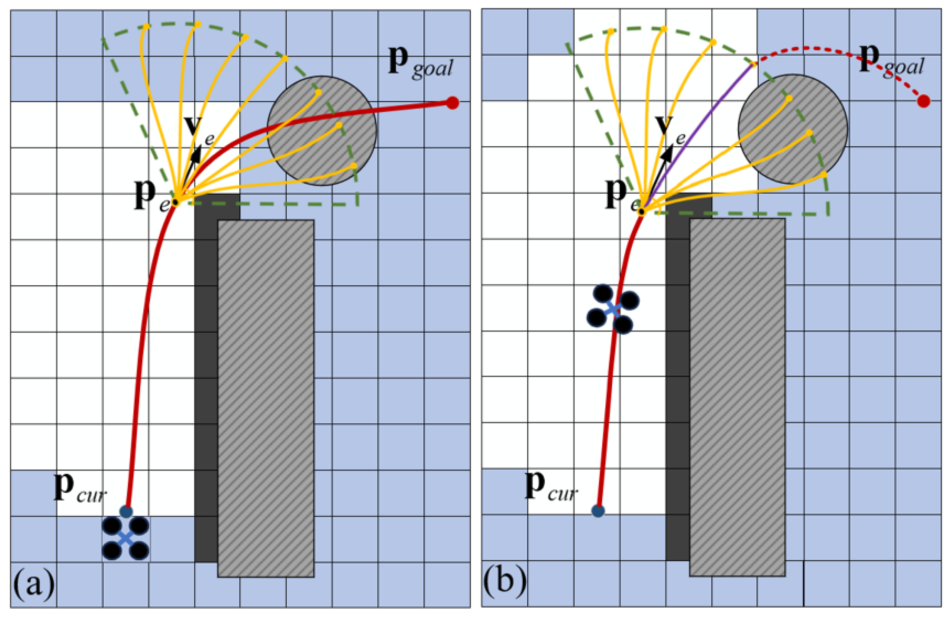
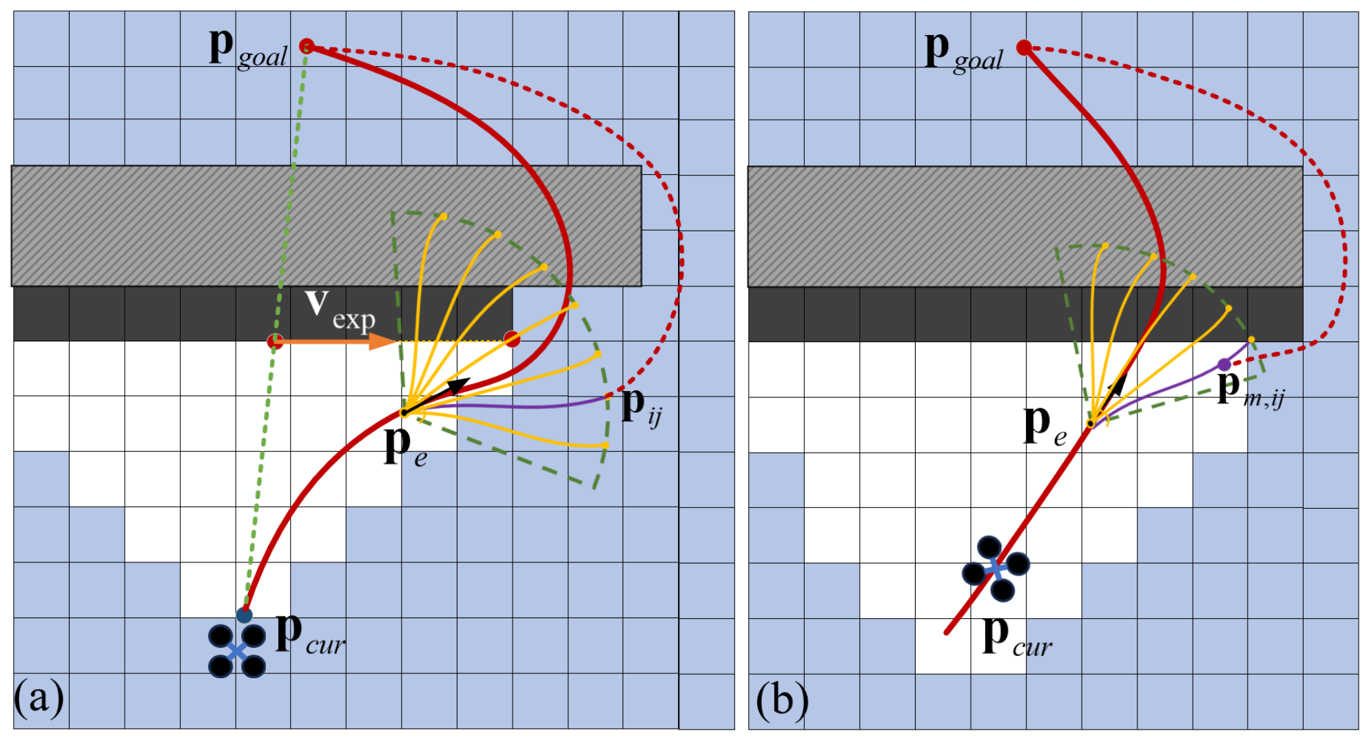
where ${\omega }_d$ is a scaling parameter. Upon completing the aforementioned steps, a set of candidate trajectories originating from ${\mathbf{p}}_e$ is obtained, as illustrated in Figure 7a.

Evaluation: All candidate trajectories are continuously evaluated prior to entering the execution stage. The time relaxation factor $t_m$ guarantees that every candidate trajectory undergoes at least one complete evaluation. For each candidate trajectory ${\mathcal{P}}_{ij}$, a position set ${\mathcal{Q}}_{ij}$ is obtained by uniformly discretizing the trajectory at a fixed time interval. The occupancy state of the grid cell corresponding to each position in ${\mathcal{Q}}_{ij}$ is queried sequentially. Upon detection of an occupied grid cell, the score of ${\mathcal{P}}_{ij}$ is immediately set to zero, and zero-scored trajectories are excluded from all subsequent evaluation iterations. Upon first encountering an unknown grid cell, or upon reaching the terminal point of the candidate trajectory, the corresponding timestamp $t_{u,ij}$ is recorded, and the trajectory score is computed according to the following formula:

$$\begin{array}{cc}\hfill F_{ij}& ={\omega }_t{f}_{t,ij}+{\omega }_g{f}_{g,ij}+{\omega }_s{f}_{s,ij}\hfill \\ \hfill f_{t,ij}& ={\displaystyle \frac{t_{u,ij}-t_e}{T_d}}\hfill \\ \hfill f_{g,ij}& ={\displaystyle \frac{d_{g,max}-d_{g,ij}}{d_{g,max}-d_{g,min}}}\hfill \\ \hfill f_{s,ij}& =1/\left(1+{\displaystyle \frac{J_{ij}}{t_{u,ij}-t_e}}\right)\hfill \end{array}$$

(11)

where $f_{t,ij}\in [0,1]$ denotes the safety score, representing the proportion of the candidate trajectory’s total duration that spent within known-free regions; $f_{g,ij}\in [0,1]$ represents the efficiency score quantifying the distance from the trajectory endpoint to ${\mathbf{p}}_{goal}$, $d_{g,ij}$ is the euclidean distance from the terminal point of the evaluated trajectory to ${\mathbf{p}}_{goal}$, $d_{g,max}$ and $d_{g,min}$ denote the maximum and minimum goal distances among all candidate trajectories, respectively; $f_{s,ij}\in [0,1]$ represents the smoothness score of the candidate trajectory; and $J_{ij}={\int }_{t_e}^{t_{u,ij}}\left|\right|jerk\left({\mathcal{P}}_{ij}\right)|{|}^{2}dt$, ${\omega }_t$, ${\omega }_g$ and ${\omega }_s$ denote the weighting coefficients corresponding to each score. In certain special cases where all candidate trajectories receive a score of zero, the pipeline transitions to the candidate trajectory evaluation procedure designated for full occlusion (in Section 3.3.2).

Execution: Prior to the drone reaching ${\mathbf{p}}_e$, the initial trajectory is continuously monitored for collisions with obstacles. If no collision is detected throughout this period, the initial trajectory is maintained and all candidate trajectories are discarded. Upon detection of a collision, the highest-scored candidate trajectory at that instant is immediately selected to replace the segment of the initial trajectory beyond ${\mathbf{p}}_e$. A new initial trajectory connecting the endpoint of the selected candidate trajectory to ${\mathbf{p}}_{goal}$ is then generated following the method described in Section 3.1, where the terminal conditions of the selected candidate trajectory serve as the initial conditions for this initial trajectory. The two trajectory segments are subsequently concatenated and dispatched to the controller for execution, after which the sensor occlusion detection algorithm resumes its cyclic operation, as illustrated in Figure 7b.

3.3.2. Strategy for Full Occlusion Conditions

In full occlusion conditions, no feasible trajectory toward the goal can be identified in the vicinity of the drone’s current position, causing the motion planner to become trapped in a local optimum and resort to blind and frequent replanning. To address this condition, the generation, evaluation, and execution pipeline developed for partial occlusion is extended and refined, with the exploration vector incorporated to enhance both the safety and efficiency of the initial trajectory.

Generation: In these scenarios, the grid cell containing ${\mathbf{p}}_{unk}$ is highly likely to be occupied, rendering the computation of trajectory visibility largely uninformative. To ensure flight safety, candidate trajectories are generated at the emergency braking safety distance. Specifically, the time interval from $t_{cur}$ to $t_{unk}$ is discretized into a decreasing sequence with a uniform time step. Starting from $t_{unk}$, the earliest timestamp $t_c$ satisfying the following condition is identified:

$${\int }_{t_i}^{t_{unk}}∥{\mathcal{P}}_{ij}^{\prime }\left(t\right)∥dt>v_{t_i}^2/2a_{max},t_i\in \{t_{unk},\dots ,t_{cur}\}$$

(12)

the term ${\int }_{t_i}^{t_{unk}}∥{\mathcal{P}}_{ij}^{\prime }\left(t\right)∥dt$ on the left-hand side of the equation denotes the length of the candidate trajectory from $t_i$ to $t_{unk}$. In implementation, the interval $[t_i,t_{unk}]$ is discretized with a sampling interval of $\Delta t_s=0.02$. The trajectory length is then approximated by accumulating the Euclidean distances between consecutive sampling points. The right-hand side $v_{t_i}^2/2a_{max}$ represents the emergency stop distance, which is the distance required to decelerate from speed $v_{t_i}$ to zero at time $t_i$. If the inequality is satisfied, it indicates that the arc length of the trajectory from the point corresponding to time $t_i$ to $t_{unk}$ is greater than the distance required for an emergency stop. In the event of an emergency, the drone can apply emergency braking by decelerating at $a_{\max }$, bringing it to a complete stop before reaching ${\mathbf{p}}_{unk}$, thereby ensuring the safety of the drone when the location of ${\mathbf{p}}_{unk}$ is unknown. Adding the temporal relaxation factor $t_m$ to $t_c$ yields the candidate trajectory generation timestamp $t_e$. Candidate trajectories are subsequently generated following the same strategy as in the partial occlusion pipeline; however, the coefficient ${\lambda }_2$ in Equation (6) is reduced to enhance the safety of trajectories in close proximity to the obstacle.

Evaluation: Since the obstacle completely blocks all nearby paths toward ${\mathbf{p}}_{goal}$, the goal-directed efficiency score term $f_{g,ij}$ not only fails to contribute any positive contribution under the current condition, but also introduces an elevated collision risk. Consequently, the exploration vector ${\mathbf{v}}_{exp}$, directed toward the boundary of the current obstacle, is adopted as the basis for candidate trajectory evaluation:

$$f_{e,ij}={\displaystyle \frac{1}{2}}\left(1-{\displaystyle \frac{{\mathbf{v}}_{\mathit{exp}}·({\mathbf{p}}_{ij}-{\mathbf{p}}_e)}{∥{\mathbf{v}}_{\mathit{exp}}∥∥({\mathbf{p}}_{ij}-{\mathbf{p}}_e)∥}}\right)$$

(13)

where $f_{e,ij}\in [0,1]$ denotes the new efficiency score, quantifying the directional alignment between the candidate trajectory and the exploration vector. The overall evaluation function is accordingly updated as follows:

$$F_{ij}={\omega }_t{f}_{t,ij}+{\omega }_e{f}_{e,ij}+{\omega }_s{f}_{s,ij}$$

(14)

Upon detecting a collision between a candidate trajectory and an obstacle, rather than immediately setting its score to zero, the collision time $t_{c,ij}$ is recorded and the following expression is evaluated:

$${\int }_{t_e}^{t_{c,ij}}∥{\mathcal{P}}_{ij}^{\prime }\left(t\right)∥dt>v_{t_{c,ij}}^2/2a_{max}$$

(15)

If the condition is satisfied, the trajectory is designated as a secondary candidate, and its safety score is updated accordingly using $t_{c,ij}$. Candidate trajectories that remain collision-free are designated as primary candidates.

Execution: When a collision is detected along the initial trajectory and at least one primary candidate trajectory exists within the candidate set, the highest-scored primary candidate is selected and executed following the partial occlusion execution strategy, as illustrated in Figure 8a. In certain special cases—for instance, when the sampling angular range is configured with a narrow field—all candidate trajectories may collide with obstacles. In such cases, the highest-scored secondary candidate is selected instead, and its effective terminal time is redefined as $t_{m,ij}=t_{c,ij}-t_q$, where $t_q$ is a time relaxation parameter. The position, velocity, and acceleration at this redefined terminal time are fed to the initial planner as initial conditions to generate a connecting trajectory toward ${\mathbf{p}}_{goal}$, as illustrated in Figure 8b.

4. Experiments and Analysis

The experimental evaluation is structured into three components: partial occlusion simulation experiments, full occlusion simulation experiments, and real-world environment experiments. The comparative methods employed include EGO-Planner [17] and CPA-Planner [24]. EGO-Planner is a well-established representative of optimistic trajectory planning, while CPA-planner builds upon Fast-Planner and addresses the safety risks in occluded unknown scenarios through a perception-aware strategy. The weighting coefficients $w_t$, $w_g$, and $w_s$ in Equation (11) are set to 0.5, 1.0, and 0.5, respectively. The weighting coefficients $w_t$, $w_e$, and $w_s$ in Equation (14) are configured as 1.0, 0.5, and 0.5, respectively. The thresholds $K_t$, $C_t$ and $R_t$ in Algorithm 1 are set to 0.25, 0.15 and 0.5, respectively. $r_{max}$ is set to 3 m; ${\lambda }_1$ and ${\lambda }_2$ in Equation (6) are set to 0.5 and 0.5 during the partial occlusion phase, and to 0.8 and 0.2 during the full occlusion phase, respectively; the temporal relaxation factors $t_m$ and $t_q$ are both set to 0.02 s; the scaling parameters ${\omega }_{\alpha }$ and ${\omega }_d$ in Equation (5) and Equation (10) are set to 0.9 and 1.2, respectively. The number of candidate trajectories is 24, the sensor perception range is 4.0 m, the resolution of the simulation map is 0.1 m, and the field-of-view angle of the drone sensor is 90°. Further details of all experiments can be accessed at the following URL: https://youtu.be/JDsDff80Vjk (accessed on 30 May 2026).

4.1. Partial Occlusion Simulation Experiments

The simulation experiments are primarily conducted using ROS Noetic on a desktop computer equipped with an Intel Core i7-12700 CPU and an NVIDIA RTX 4090 GPU, running Ubuntu 20.04. The simulation experiments in Section 4.2 are built upon the same configuration.

4.1.1. Operational Process Analysis

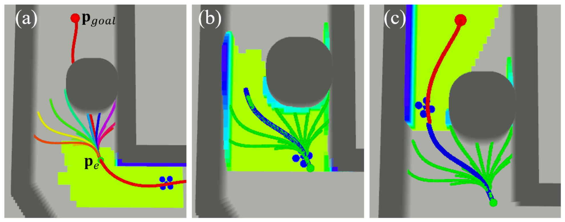
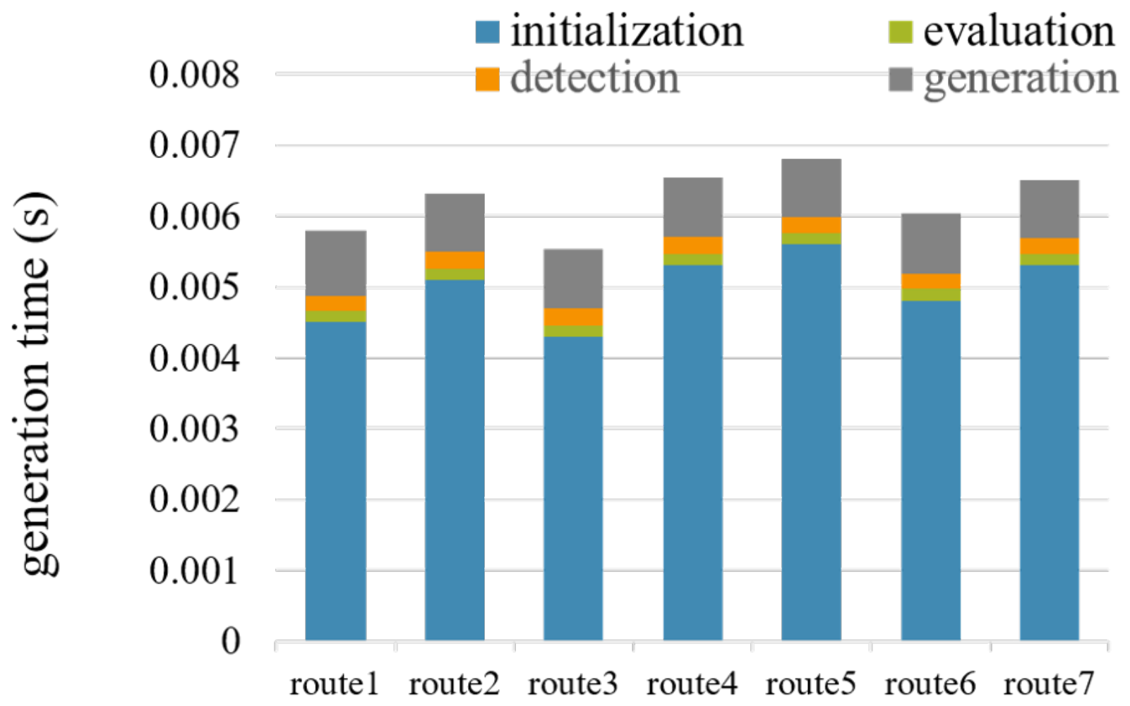
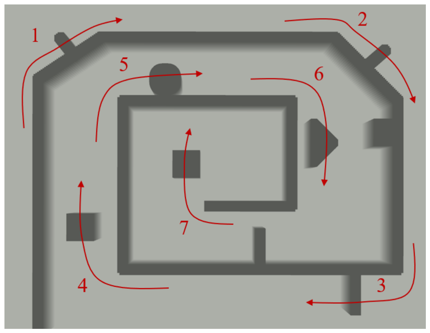
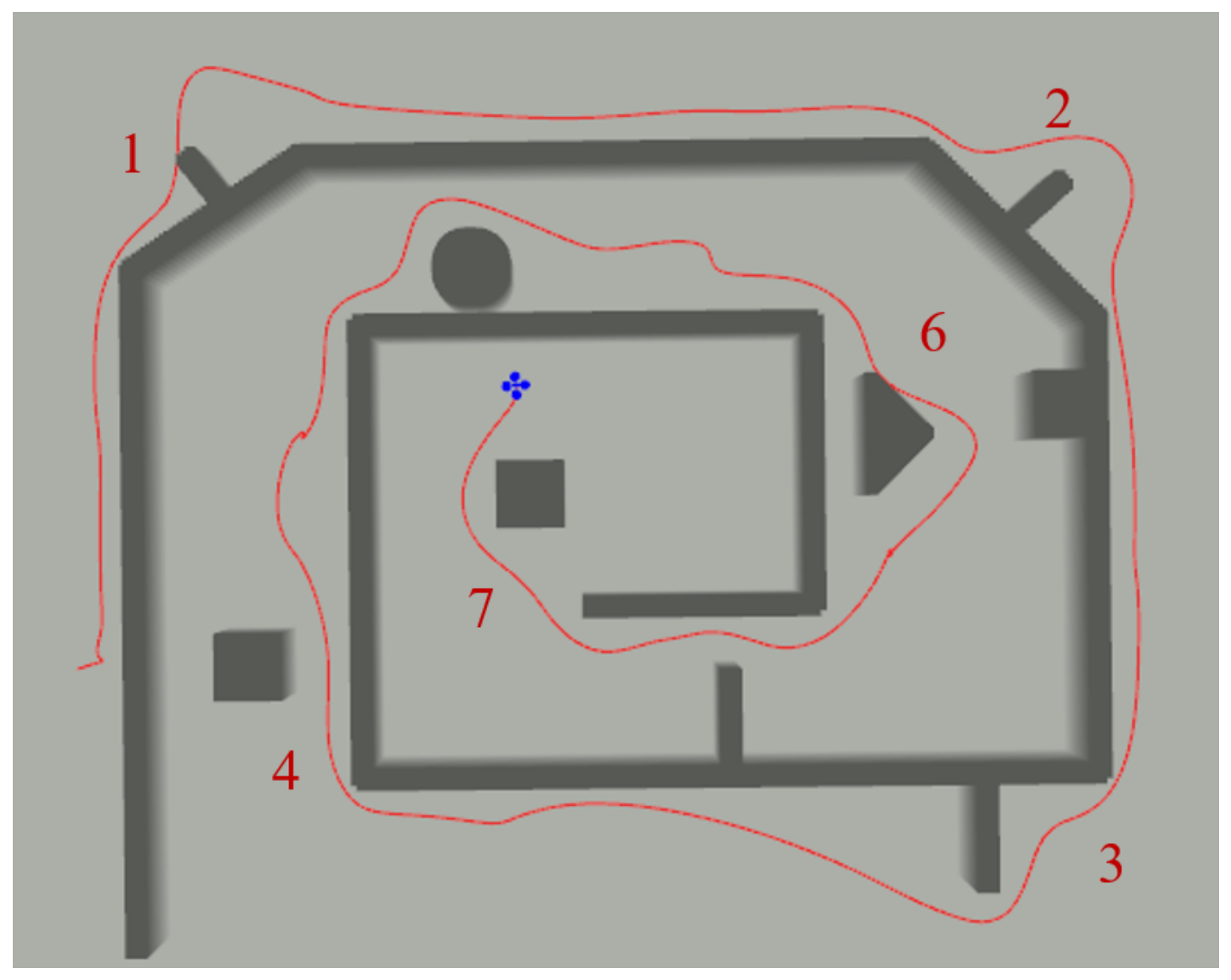
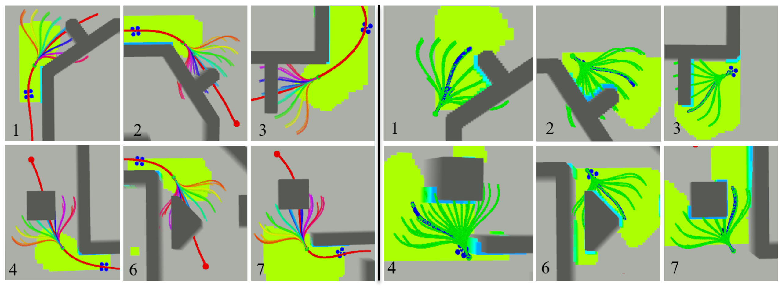
The simulation environment is constructed as illustrated in Figure 9. The experimental scenario comprises seven routes, simulating partial occlusion conditions of varying degrees encountered by the drone when navigating turns in indoor corridors. The maximum flight velocity is set to 5 m/s. The operational execution of the proposed method is first analyzed using Route 5 as a representative case, as illustrated in Figure 10. Figure 10a demonstrates the sensor occlusion detection algorithm detecting a partial occlusion condition, generating color-coded candidate trajectories at ${\mathbf{p}}_e$. Figure 10b illustrates the candidate trajectory evaluation and execution stage: after detecting a collision between the initial trajectory and an obstacle, the planner switches to a candidate trajectory, with the blue trajectory indicating the highest-scored candidate. Figure 10c illustrates the initial trajectory connecting the terminal point of the selected candidate trajectory to the goal point. Figure 11 illustrates the overall flight trajectory of the proposed method in the partial-occlusion simulation experiments. Figure 12 presents screenshots captured at the moment of candidate trajectory generation along each route, as well as screenshots taken when the candidate trajectory with the highest score is selected for execution. Figure 13 presents a comparison of computation time among initial trajectory planning, candidate trajectory generation, candidate trajectory evaluation, and sensor occlusion detection. The execution of candidate trajectories—forwarding the selected optimal candidate trajectory to the controller—involves no additional computation and completes nearly instantaneously; it is therefore not included in the statistics shown in the Figure 13. As observed from the figure, the time consumed by sensor occlusion detection and candidate trajectory evaluation in the proposed algorithm is considerably smaller than that consumed by candidate trajectory generation. Furthermore, since candidate trajectory generation employs a closed-form solution and does not account for obstacle collision during generation, its computation time is considerably smaller than that of initial trajectory generation.

4.1.2. Comparative Analysis

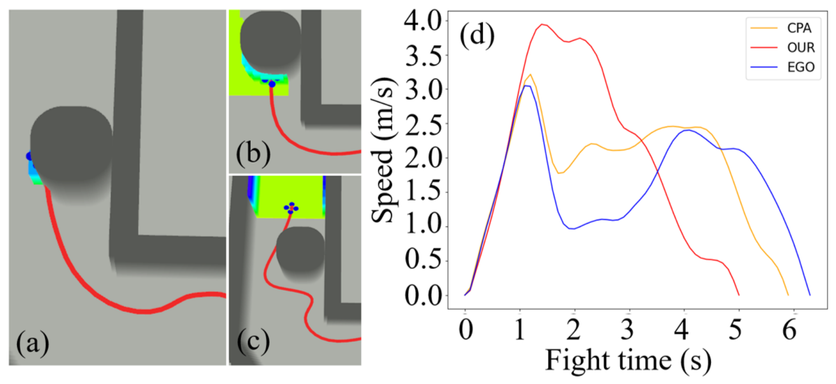
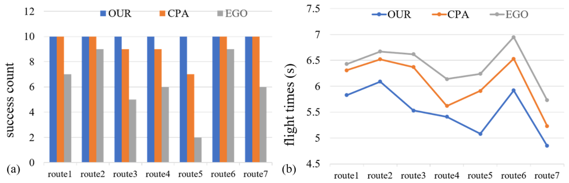
All compared methods are evaluated over 10 trials per route, with any collision occurrence classified as a failure. The success counts are summarized in Figure 14a. The proposed method achieves a 100% success rate across all routes. CPA-planner also demonstrates a high success rate, with only a few collision failures occurring on Routes 3, 4, and 5. EGO-Planner experiences collisions on most routes due to its limited capacity to handle occluded obstacles. Figure 14b presents a comparison of the mean traversal time of all evaluated methods across each route. The proposed method achieves the shortest time across all routes. To enhance trajectory visibility, CPA-planner elongates the trajectory prior to entering occluded areas, which inevitably increases traversal time. In contrast, the proposed method preserves the initial trajectory without modification and incorporates smoothness and efficiency scores as evaluation metrics during candidate trajectory selection, enabling more agile and efficient flight. EGO-Planner, suffers from frequent trajectory replanning triggered by sudden obstacle detection, resulting in prolonged traversal times due to repeated deceleration and re-optimization cycles.

Table 1. Performance in partial occlusion scenes.

Methods	Metrics	Route 1	Route 2	Route 3	Route 4	Route 5	Route 6	Route 7
Ours	ATL (m)	11.64	12.15	10.97	10.82	10.16	11.84	9.63
	STL (m)	0.2035	0.2317	0.1942	0.2461	0.2087	0.2918	0.1853
	SFT (s)	0.1031	0.1197	0.0924	0.1197	0.0959	0.1493	0.0817
	ART (ms)	1.51	1.47	1.49	1.45	1.43	1.47	1.52
	SRT (ms)	0.0403	0.0359	0.0297	0.0327	0.0415	0.0337	0.0416
EGO- planner	ATL (m)	12.25	12.93	11.59	11.15	11.58	12.43	10.37
	STL (m)	0.3428	0.2705	0.4418	0.3671	0.7200	0.3152	0.5371
	SFT (s)	0.1957	0.1529	0.2104	0.1798	0.3850	0.1549	0.2439
	ART (ms)	1.24	1.31	1.25	1.12	1.32	1.25	1.53
	SRT (ms)	0.1704	0.1425	0.1876	0.1439	0.1928	0.1342	0.1503
CPA- planner	ATL (m)	11.89	12.57	11.35	11.18	10.98	12.11	10.04
	STL (m)	0.2451	0.2349	0.2176	0.2613	0.3145	0.2392	0.1931
	SFT (s)	0.1295	0.1227	0.1137	0.1259	0.1393	0.1206	0.1039
	ART (ms)	3.45	3.32	3.17	3.53	3.51	3.24	3.47
	SRT (ms)	0.3629	0.3145	0.2975	0.3596	0.4107	0.3258	0.3173

presents the detailed quantitative results of each algorithm in the comparative experiments. In the table, ATL denotes average trajectory length, STL denotes standard deviation of trajectory length, SFT denotes standard deviation of flight time, ART denotes average replanning time, and SRT denotes standard deviation of replanning time. As shown in the table, our algorithm achieves the smallest ATL, STL, and SFT among all compared methods, demonstrating that it not only provides more efficient trajectories but also exhibits stronger robustness. EGO-Planner, as a method primarily designed for computational efficiency, achieves the shortest average replanning time. The replanning time of the proposed method is not substantially different from that of EGO-Planner and is considerably shorter than that of CPA-Planner. Moreover, since the replanning process of the proposed method does not involve repeated iterations or other optimization procedures with substantial uncertainty, the replanning time exhibits strong stability. Figure 15a–c presents the collision incidents recorded for CPA-planner and EGO-Planner during experiments on Route 5, while Figure 15d illustrates the comparative speed profiles of all evaluated methods throughout Route 5.

4.2. Full Occlusion Simulation Experiments

4.2.1. Operational Process Analysis

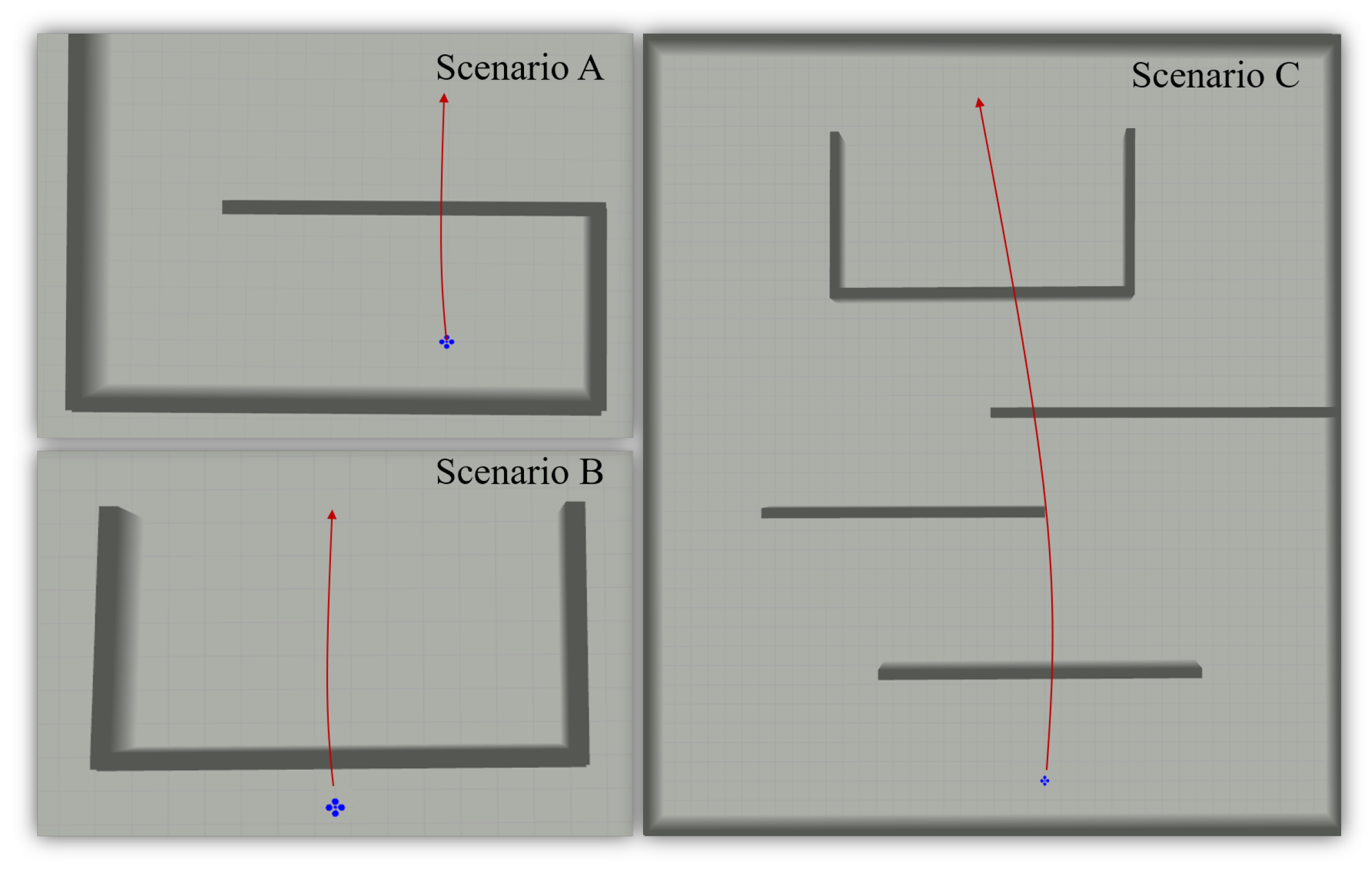
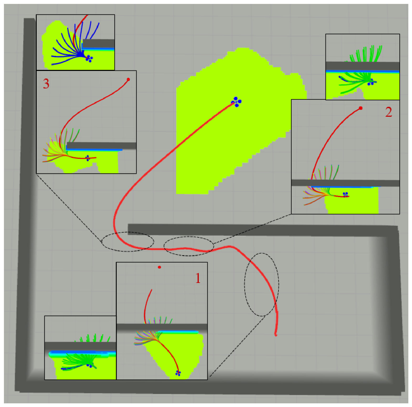
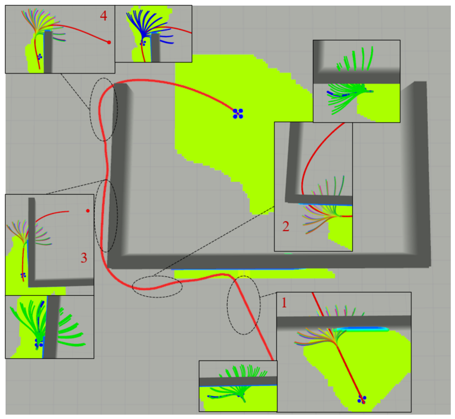
Three experimental scenarios are designed for the full occlusion case, as illustrated in Figure 16. Specifically, Scenario A and Scenario B represent single-obstacle simulations targeting two distinct wall configurations, while Scenario C represents a complex multi-wall indoor environment simulation. The maximum flight altitude is constrained to 3 m, and the maximum flight velocity is set to 4 m/s. Two single-obstacle scenarios are first presented as illustrative examples to analyze in detail the execution process of the proposed method under full occlusion conditions. As illustrated in Figure 17: the proposed method performs a total of three times of candidate trajectory generation in Scenario A. In the first two instances, the sensor occlusion detection algorithm classifies the scene as full occlusion, whereupon the corresponding candidate trajectory generation, evaluation, and execution pipeline is carried out accordingly. In the third instance, the scene is classified as partial occlusion. Furthermore, no collision between the initial trajectory and any obstacle is detected during the execution stage, and consequently all candidate trajectories are discarded without execution—reflected in the figure by all candidate trajectories being rendered in blue. As illustrated in Figure 18, the proposed method performs a total of four rounds of candidate trajectory generation throughout the execution process in Scenario B. Among these, the first three rounds are triggered under full occlusion conditions, while the fourth round is triggered under partial occlusion conditions, with no candidate trajectory ultimately selected for execution.

To investigate the influence of different score terms in the candidate trajectory evaluation function on the algorithm’s performance, a weight sensitivity analysis is designed for each score weight. In scenario A, the effect of different weight values on the algorithm’s performance is examined by varying one weight at a time while holding the other two fixed. Each parameter configuration is tested over 10 trials, and the results are presented in the

Table 2. Results in scenario A under different $w_t$ values ($w_s$ = 0.5, $w_e$ = 0.5).

Value of ${\mathit{w}}_{\mathit{t}}$	0	0.1	0.5	1.0	2.0	10	100
Number of success	0	5	10	10	10	8	7
Trajectory Length (m)	/	19.73	20.75	20.63	21.35	25.49	30.43
Flight Time (s)	/	8.73	9.03	8.93	9.23	13.26	20.87

,

Table 3. Results in scenario A under different $w_e$ values ($w_t$ = 1.0, $w_s$ = 0.5).

Value of ${\mathit{w}}_{\mathit{e}}$	0	0.1	0.3	0.5	1.0	10	100
Number of success	7	10	10	10	10	5	0
Trajectory Length (m)	31.89	24.56	21.92	20.63	20.47	20.81	\
Flight Time (s)	20.83	13.82	9.13	8.93	8.83	9.35	\

and

Table 4. Results in scenario A under different $w_s$ values ($w_t$ = 1.0, $w_e$ = 0.5).

Value of ${\mathit{w}}_{\mathit{s}}$	0	0.1	0.5	1.0	10	30	100
Number of success	10	10	10	10	10	7	1
Trajectory Length (m)	21.08	20.53	20.63	20.74	21.47	25.68	\
Flight Time (s)	9.23	9.06	8.93	9.15	9.34	12.65	\

.

Table 2 presents the sensitivity analysis results for $w_t$. As observed, when $w_t$ is set to 0, the evaluation of candidate trajectories completely ignores safety factors, rendering the trajectories unable to avoid collisions with obstacles, which results in zero successful trials. When $w_t$ is set to 0.1, the success rate improves immediately. However, since $w_e$ and $w_s$ are relatively higher than $w_t$, the planned trajectories tend to closely hug the obstacles. Although the trajectory efficiency is high, the safety remains compromised. Varying $w_t$ between 0.5 and 2.0 has little noticeable effect on the algorithm’s performance. Nevertheless, when $w_t$ is set excessively large, variations in the safety score dominate over variations in the efficiency score, preventing the algorithm from escaping local optima through the exploration vector.

Table 3 shows the sensitivity analysis results for $w_e$. When $w_e$ is set to 0, trajectory evaluation entirely neglects efficiency, making the algorithm unable to locate obstacle boundaries through the exploration vector. The planner occasionally fails due to getting trapped in local optima. Improving $w_e$ to 0.1 enables the planner to escape local optima. However, because $w_e$ constitutes a relatively small proportion compared to $w_s$ and $w_t$, the candidate trajectories cannot guarantee optimal efficiency. The algorithm achieves satisfactory performance when $w_e$ ranges from 0.3 to 1.0. Conversely, an excessively large $w_e$ causes the candidate trajectory evaluation to be dominated solely by the exploration vector, thereby compromising trajectory safety.

Table 4 shows the sensitivity analysis results for $w_s$. It can be observed that the algorithm’s performance does not fluctuate substantially as $w_s$ varies between 0 and 10. This is because the sensor employed in the experiments has a field of view of 90°, within which all generated candidate trajectories satisfy the dynamic feasibility constraints and remain smooth, with no substantial differences in the integrated jerk. Therefore, as long as $w_s$ is not set excessively large, it does not have a significant impact on the algorithm’s performance. However, if a sensor with a wider field of view were adopted, the effect of $w_s$ would become more pronounced. If $w_s$ is set excessively large, it would dominate over the safety score, compromising the guarantee of trajectory safety.

To examine the performance of the proposed algorithm under different flight speeds, experiments are conducted in scenario B with maximum speeds set to 3 m/s, 4 m/s, and 5 m/s, respectively, with each speed condition tested over 10 trials. The statistical results of the proposed algorithm under each speed condition are summarized in

Table 5. Results of the proposed method in scenario B under different velocities.

Max Speed	Num. of Success	Avg. Traj. Length (m)	Max Traj. Length (m)	Avg. Flight Times (s)	Max Flight Times (s)
3 m/s	10	24.97	28.63	14.39	16.74
4 m/s	10	25.84	29.06	11.26	14.51
5 m/s	8	27.04	31.72	9.54	13.19

. As shown in the Table 5, two collisions occur in the experiments when the velocity is set to 5 m/s. While the exploration vector can guide candidate trajectories toward obstacle boundaries, multiple candidate segments must be connected to the original initial trajectory. In the two failed trials, collisions occur during the subsequent initial trajectory phase after the candidate trajectories are executed. Under full occlusion, the drone is required to perform frequent replanning continuously around the obstacle. Increasing the maximum velocity reduces the time allocated by the planner to each trajectory segment, causing the trajectory shape to become more aggressive and thereby increasing the risk of collision. Adopting a safer initial trajectory planning algorithm would enhance the performance of the proposed framework under high-speed conditions.

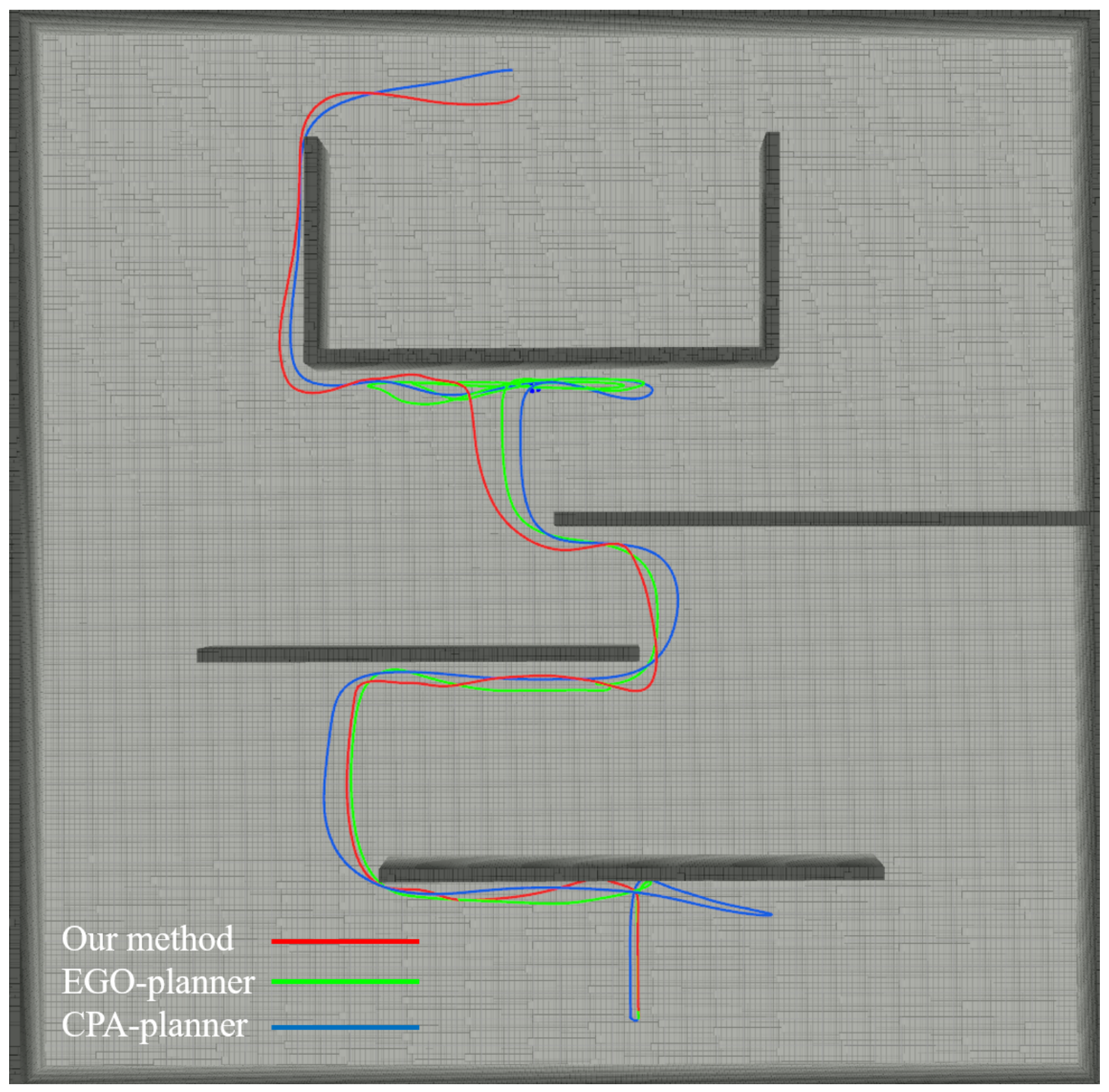
4.2.2. Comparative Analysis

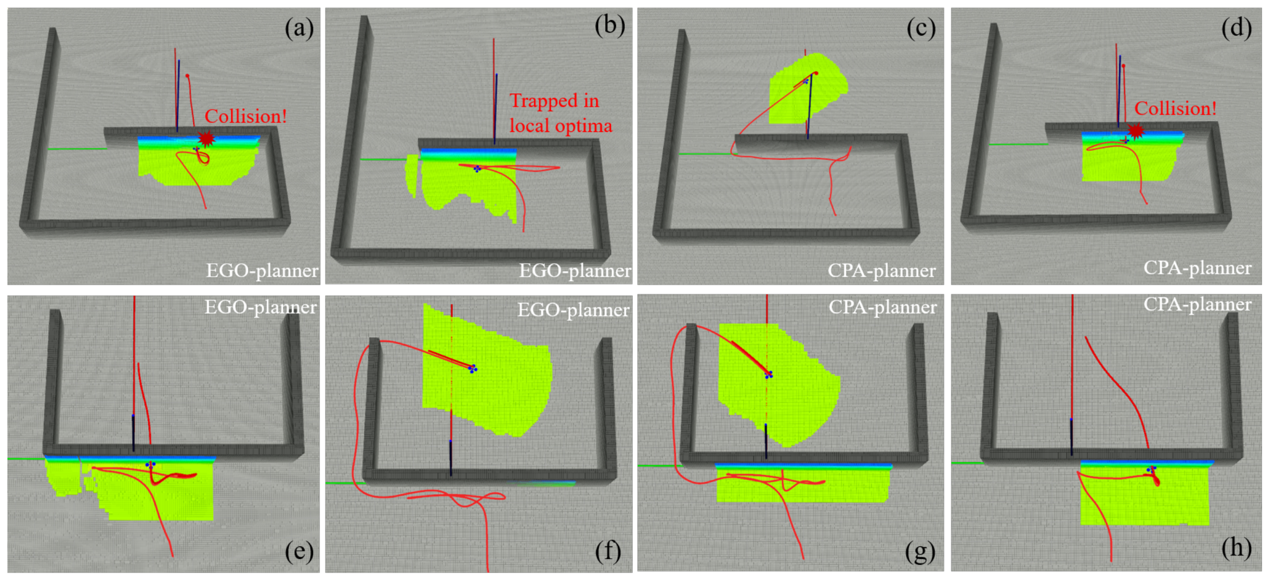
All methods are evaluated over ten trials in each of the three scenarios. Figure 19 presents the execution results of EGO-Planner and CPA-Planner in single-obstacle Scenario A and Scenario B. Figure 20 presents a comparative illustration of the trajectories generated by the proposed algorithm and the two baseline algorithms in Scenario C. EGO-Planner and CPA-planner exhibit comparable behavior in full occlusion scenarios, both manifesting highly unstable flight performance. In certain trials, these methods result in collisions, while in others, they reach the goal safely only after executing substantial detours. Neither EGO-planner nor CPA-planner incorporates global information during trajectory planning; consequently, both fail to effectively avoid local optima under conditions of complete occlusion. In contrast, the proposed algorithm identifies full occlusion scenarios via the sensor occlusion detection algorithm, and rapidly escapes local optima by selecting the highest-scoring candidate trajectory guided by the exploration vector.

Table 6. Performance in full occlusion scenes.

Scenarios	Method	Avg. Traj. Length (m)	Avg. Flight Times (s)	Num. of Success	Std. Flight Times (s)	Std. Traj. Length (m)
scenario A	our method	20.63	8.93	10	0.76	1.68
	CPA-planner	29.54	18.73	8	2.31	3.51
	EGO-planner	33.71	21.53	7	3.08	4.43
scenario B	our method	25.84	11.26	10	0.85	1.83
	CPA-planner	34.41	23.54	7	3.25	4.56
	EGO-planner	36.93	27.83	5	4.17	5.31
scenario C	our method	75.25	31.47	10	1.73	2.85
	CPA-planner	95.76	58.62	5	5.63	9.31
	EGO-planner	/	/	1	/	/

summarizes the statistical results of all methods across all three experimental scenarios. As can be observed from the table, the proposed algorithm achieves optimal performance in terms of trajectory length, flight time, and success rate. EGO-Planner exhibits the poorest overall performance; in Scenario C, it successfully reached the goal in only one trial after an extensively prolonged detour, while the remaining trials resulted in either collisions with obstacles or entrapment in local optima (quantitative statistics for EGO-Planner in Scenario C are not included in the table).

4.3. Real-World Experiments

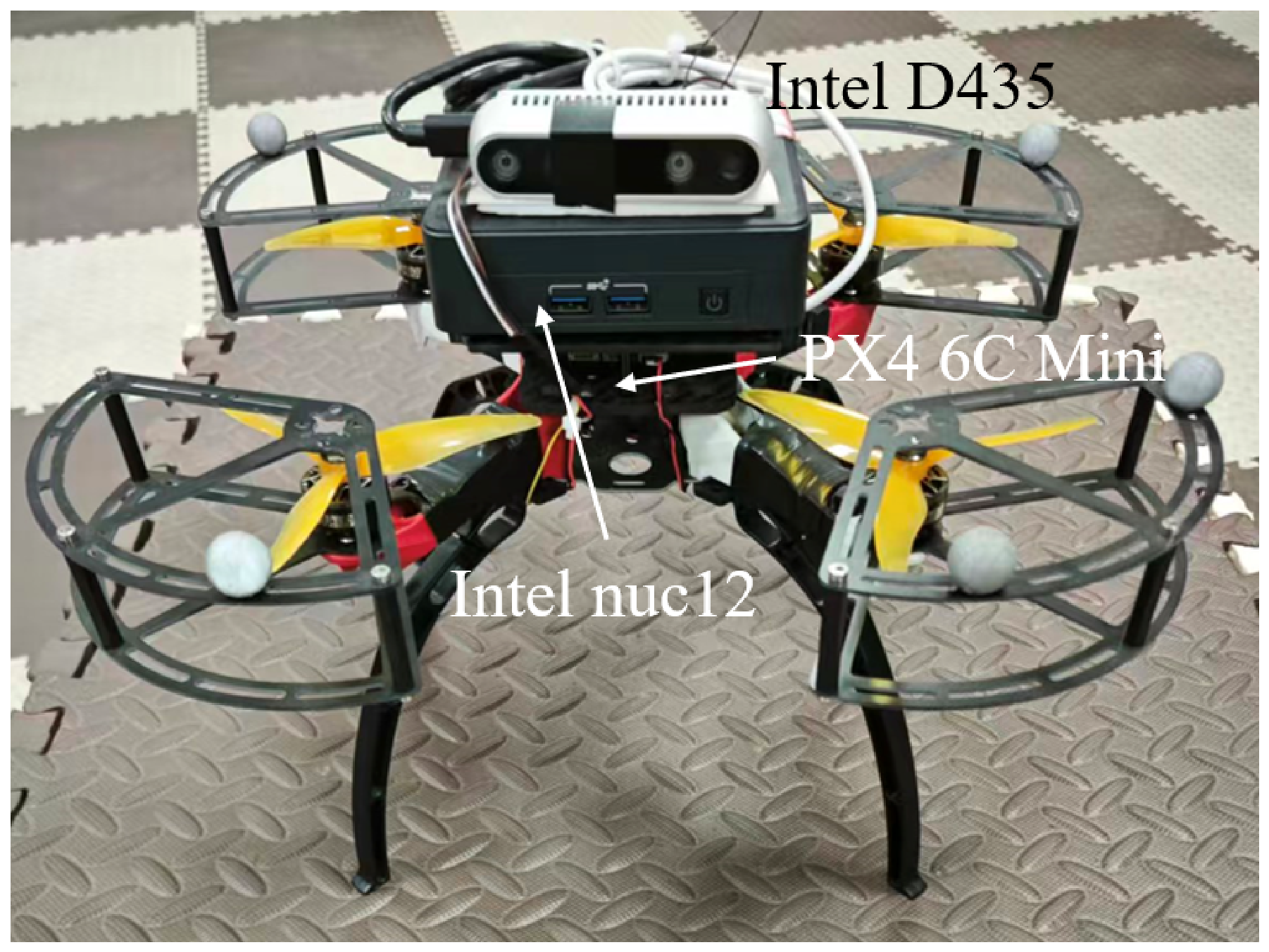
To further validate the effectiveness of the proposed method, real-world flight experiments were conducted under sensor occlusion conditions. The quadrotor platform used in the experiments is shown in Figure 21, which is equipped with an Intel RealSense D435 depth camera as the onboard sensor, a Pixhawk 6C Mini as the flight controller, and an Intel NUC12 as the onboard computer. The onboard computing environment runs Ubuntu 20.04 and ROS Noetic. The experimental site is a 6.6 m × 7.8 m square room. During the experiments, the maximum velocity of the quadrotor is set to 3 m/s, and a motion capture system is employed to provide accurate localization for the quadrotor.

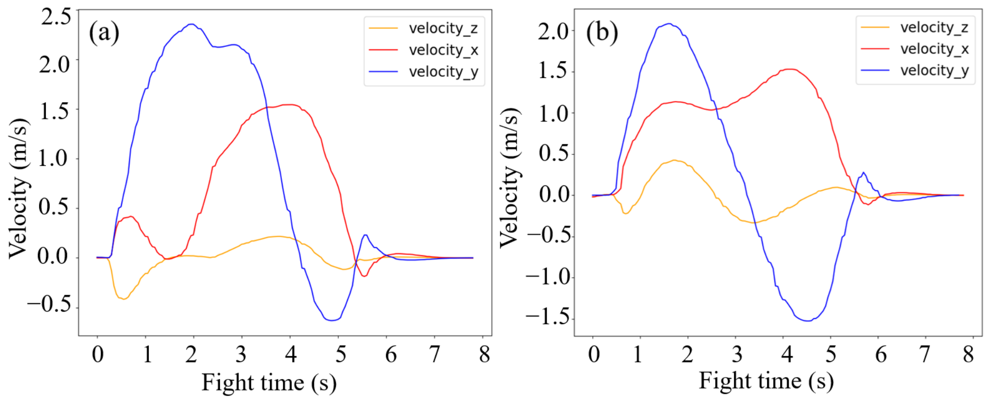
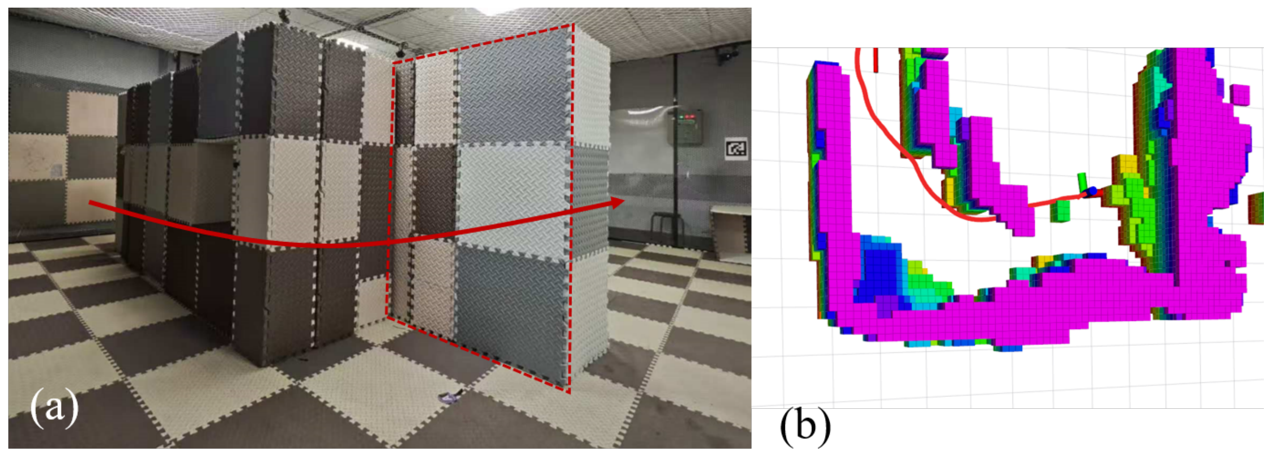
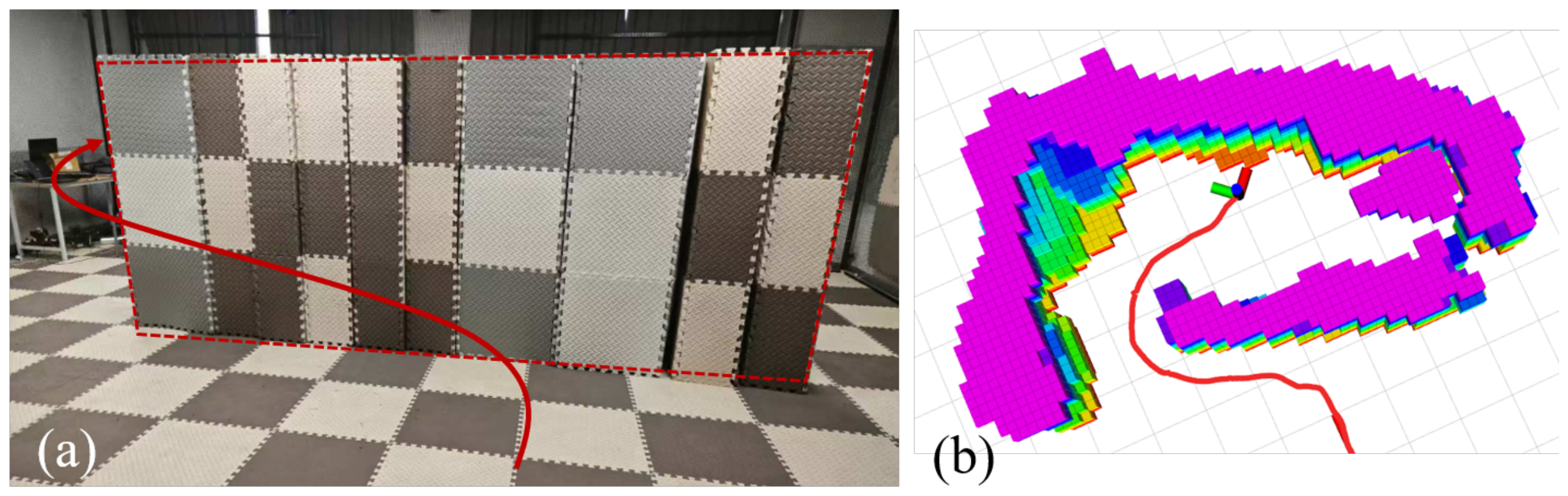
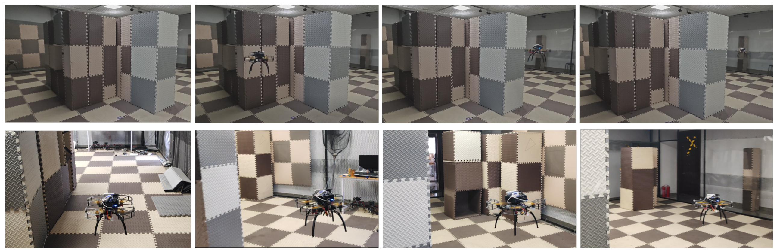
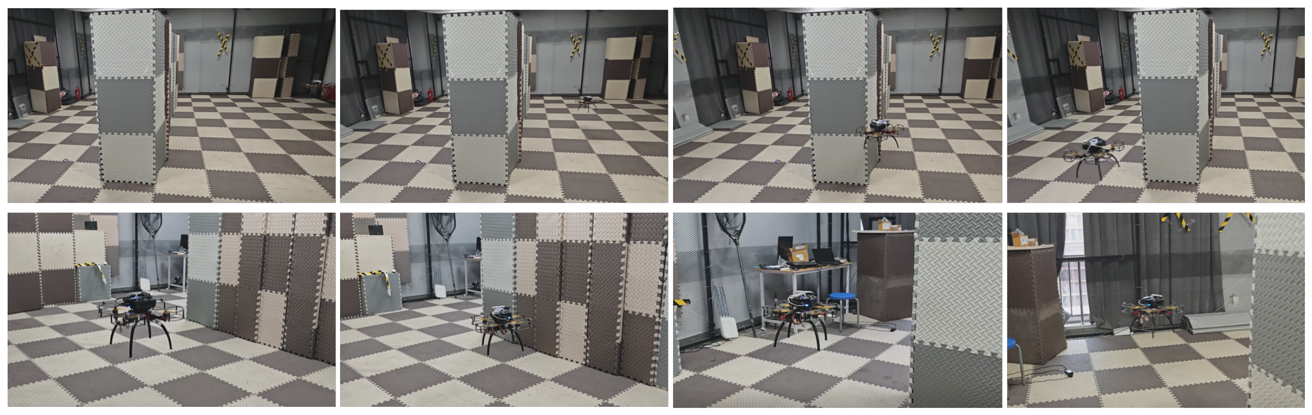
The partial occlusion experimental scenario is illustrated in Figure 22a, which simulates a quadrotor navigating an indoor corridor turn, where the obstacle highlighted by the red bounding box is occluded from the sensor’s field of view. Figure 22b presents the 3D occupancy grid map constructed by the quadrotor and the corresponding flight trajectory recorded during the experiment. The full occlusion experimental scenario is shown in Figure 23a, simulating a condition in which the quadrotor’s sensor field of view is completely blocked by an indoor wall. Figure 23b presents the 3D occupancy grid map and flight trajectory recorded during a representative trial of this scenario. Ten trials are conducted in each of the two experimental scenarios, and the statistical results are summarized in

Table 7. Performance in real-world experiments.

	Avg. Traj. Length (m)	Avg. Flight Times (s)	Std. Traj. Length (m)	Std. Flight Times (s)	Number of Success
partial occlusion	8.73	5.54	0.2416	0.1672	10
full occlusion	9.34	6.08	0.2953	0.2094	10

. As shown in the table, the proposed method achieves a 100% success rate across both occlusion scenarios in real-world experiments. Figure 24 and Figure 25 present snapshots of the quadrotor at various positions recorded during the partial occlusion and full occlusion experiments, respectively. Figure 26 illustrates the velocity profiles obtained from a representative trial in each of the two scenarios.

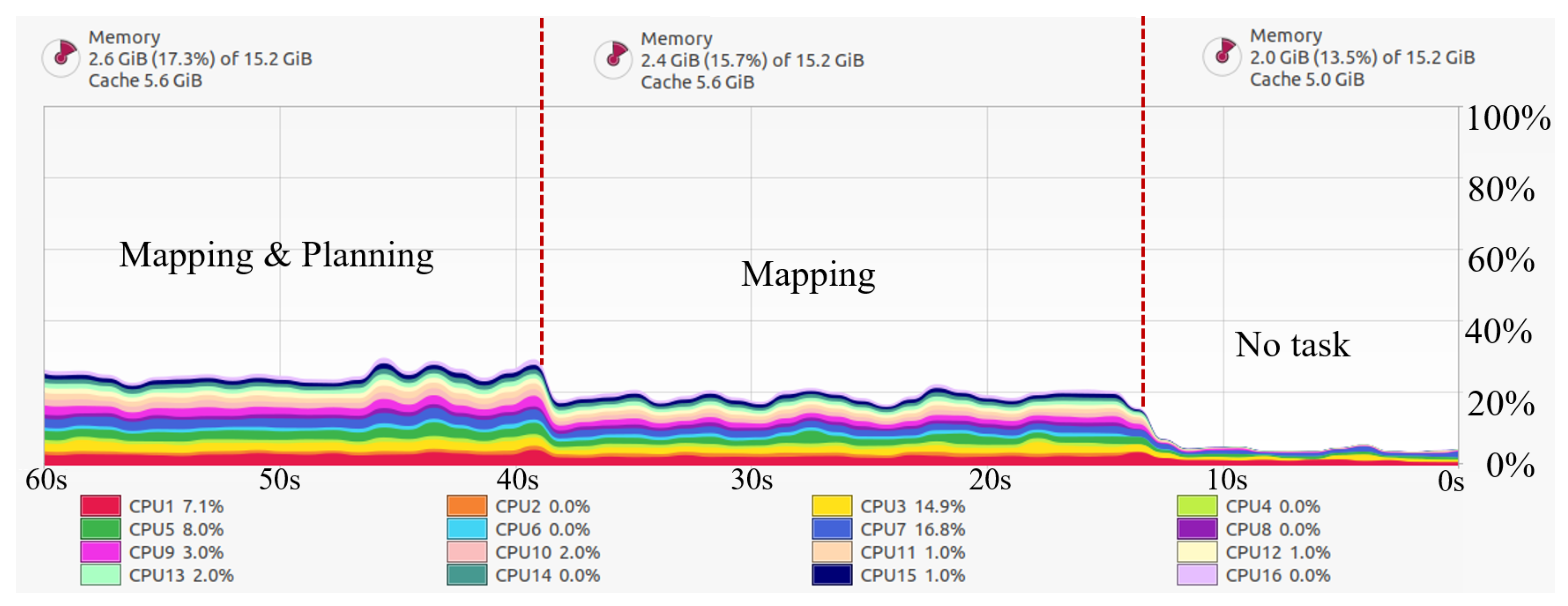
Figure 27 presents the CPU usage curve and memory usage pie chart recorded during one trial of the partial-occlusion experiment. The computational resource consumption in the full-occlusion experiment is highly similar to that of the partial-occlusion experiment and is therefore not shown separately. The CPU model is an Intel Core i7-1260P (Intel, Santa Clara, CA, USA). As shown in the figure, the CPU utilization of the proposed framework remains below 25% during actual operation. Among the computational components, map updating to maintain the surrounding environment constitutes the primary computational overhead, whereas the CPU resources required by the proposed planning framework are comparatively modest. In terms of memory usage, under the conditions of a perception range of 4.5 m and a map resolution of 0.1 m, the memory consumed by map construction is approximately 400 MB, while that required to run the proposed planning algorithm is approximately 200 MB. The computational and memory resources demanded by the proposed algorithm are both low, enabling reliable operation even on onboard computers with relatively limited processing capability. The real-world experiments further validate the effectiveness of the proposed method.

5. Discussion and Conclusions

5.1. Limitations in Practical Applications

In the real-world experiments, a motion capture system was employed to provide pose information for the drones so as to eliminate confounding factors and evaluate the proposed planning framework with greater precision. In practice, however, the pose estimates available onboard a drone typically fall short of the accuracy and stability provided by a motion capture system and are subject to errors of varying magnitude. For example, when a visual-SLAM framework such as VINS-Fusion is adopted for pose estimation, the proposed algorithm remains capable of delivering reasonably reliable performance provided that the localization error stays within 0.5 m. As drift errors gradually accumulate, however, the probability that the optimal candidate trajectory selected by the evaluator collides with obstacles increases progressively. Therefore, in indoor environments—particularly in scenes dominated by white walls with limited texture features—the integration of a LiDAR sensor is recommended to achieve higher localization accuracy.

The candidate trajectory generation range of the proposed algorithm is directly related to the sensor’s perception range. In the case of full occlusion, a camera with an excessively narrow field of view may result in the absence of any collision-free trajectory that satisfies the required constraints among the candidate trajectories. In the real-world experiments, a RealSense D435 camera (Intel, Santa Clara, CA, USA) with an 87° field of view is employed, yielding favorable results. If alternative cameras are utilized, a field-of-view greater than 80° is recommended to ensure robust algorithm performance under full occlusion conditions. Additionally, the initial trajectory planning algorithm affects the framework’s performance in full occlusion scenarios. The EGO-planner adopted in this work guarantees flight safety at a maximum velocity of 4 m/s. To further increase the maximum flight speed, it is necessary to employ a more robust initial trajectory planner.

Currently, the proposed algorithm considers trajectory planning exclusively for static obstacles in conventional indoor environments. In scenarios where the navigable region is extremely narrow, or where moving objects such as pedestrians are present in the occluded area, the proposed algorithm cannot guarantee trajectory planning safety. We plan to investigate drone trajectory planning in the presence of pedestrians moving within occluded regions as part of our future work.

5.2. Conclusions

This article investigates the problem of sensor occlusion caused by obstacles during autonomous indoor flight of drones and proposes a novel trajectory planning framework to enhance flight safety and efficiency under such conditions. The framework first generates an initial trajectory through A-star path search and B-spline curve optimization. A sensor occlusion detection algorithm is then applied to classify scenarios in which the trajectory enters unknown regions into three categories: occlusion-free, partial occlusion, and full occlusion. For occlusion-free scenarios, execution of the initial trajectory proceeds without modification. In partial occlusion scenarios, the occlusion-aware trajectory replanning algorithm enhances drone flight safety and efficiency. The algorithm first samples multiple candidate trajectories within unknown regions, then evaluates them using a composite scoring function encompassing safety, efficiency, and smoothness. Upon detection of a collision along the initial trajectory, the highest-scoring candidate trajectory is substituted for the initial trajectory. For full occlusion scenarios, an exploration vector is additionally introduced to rapidly identify boundary points of the obstacle and escape local optima. Comprehensive simulation experiments were designed to evaluate the performance of the proposed algorithm under both partial and full occlusion scenarios, with comparative evaluations conducted against EGO-Planner and CPA-Planner. The comparative results demonstrate the effectiveness of the proposed algorithm. Furthermore, real-world occlusion experimental scenarios were constructed to further validate the practical feasibility of the proposed method.

In future work, we will continue to investigate the sensor occlusion problem and plan to address it through multi-drone cooperative planning strategies. Swarm systems can provide a broader collective perception range, thereby further enhancing the safety and efficiency of drone flight.

References

1. Xiong, H.; Yu, B.; Zhang, Y. Research on autonomous navigation and obstacle avoidance methods for high-speed large-inertia rotor UAV. Drones 2026, 10, 259. [Google Scholar]
2. Cheng, Z.; Yang, J.; Sun, J.; Zhao, L. Trajectory planning of unmanned aerial vehicles in complex environments based on intelligent algorithm. Drones 2025, 9, 468. [Google Scholar] [CrossRef] [Scilit]
3. Xu, L.; Zhang, K.; Jiang, B. Re-Planning of Reconnaissance Missions for Multi-UAV Systems Under Potential Faults. In Proceedings of the 2025 4th Conference on Fully Actuated System Theory and Applications (FASTA), Nanjing, China, 4–6 July 2025; IEEE: Piscataway, NJ, USA, 2025; pp. 923–928. [Google Scholar]
4. Menouar, H.; Guvenc, I.; Akkaya, K.; Uluagac, A.S.; Kadri, A.; Tuncer, A. UAV-enabled intelligent transportation systems for the smart city: Applications and challenges. IEEE Commun. Mag. 2017, 55, 22–28. [Google Scholar] [CrossRef] [Scilit]
5. Huang, H.; Su, J.; Wang, F.-Y. The potential of low-altitude airspace: The future of urban air transportation. IEEE Trans. Intell. Veh. 2024, 9, 5250–5254. [Google Scholar] [CrossRef] [Scilit]
6. Long, Y.; Xu, G.; Zhao, J.; Xie, B.; Fang, M. Dynamic truck–UAV collaboration and integrated route planning for resilient urban emergency response. IEEE Trans. Eng. Manag. 2024, 71, 9826–9838. [Google Scholar]
7. Zhai, Y.; Reiter, R.; Scaramuzza, D. PA-MPPI: Perception-aware model predictive path integral control for quadrotor navigation in unknown environments. IEEE Robot. Autom. Lett. 2026, 11, 3804–3811. [Google Scholar] [CrossRef] [Scilit]
8. Zhou, X.; Wen, X.; Wang, Z.; Gao, Y.; Li, H.; Wang, Q.; Yang, T.; Lu, H.; Cao, Y.; Xu, C.; et al. Swarm of micro flying robots in the wild. Sci. Robot. 2022, 7, 5954. [Google Scholar] [CrossRef] [Scilit]
9. Nieuwenhuisen, M.; Behnke, S. Search-based 3D planning and trajectory optimization for safe micro aerial vehicle flight under sensor visibility constraints. In Proceedings of the 2019 IEEE International Conference on Robotics and Automation (ICRA), Montreal, QC, Canada, 20–24 May 2019; IEEE: Piscataway, NJ, USA, 2019; pp. 9123–9129. [Google Scholar]
10. Lopez, B.T.; How, J.P. Aggressive 3-D collision avoidance for high-speed navigation. In Proceedings of the 2017 IEEE International Conference on Robotics and Automation (ICRA), Singapore, 29 May–3 June 2017; IEEE: Piscataway, NJ, USA, 2017; pp. 5759–5765. [Google Scholar]
11. Liu, T.; Wang, Q.; Zhong, X.; Wang, Z.; Xu, C.; Zhang, F.; Gao, F. Star-convex constrained optimization for visibility planning with application to aerial inspection. In Proceedings of the 2022 IEEE International Conference on Robotics and Automation (ICRA), Philadelphia, PA, USA, 23–27 May 2022; IEEE: Piscataway, NJ, USA, 2022; pp. 7861–7867. [Google Scholar]
12. Liu, S.; Watterson, M.; Mohta, K.; Sun, K.; Bhattacharya, S.; Taylor, C.J.; Kumar, V. Planning dynamically feasible trajectories for quadrotors using safe flight corridors in 3-D complex environments. IEEE Robot. Autom. Lett. 2017, 2, 1688–1695. [Google Scholar] [CrossRef] [Scilit]
13. Chen, J.; Liu, T.; Shen, S. Online generation of collision-free trajectories for quadrotor flight in unknown cluttered environments. In Proceedings of the 2016 IEEE International Conference on Robotics and Automation (ICRA), Stockholm, Sweden, 16–21 May 2016; IEEE: Piscataway, NJ, USA, 2016; pp. 1476–1483. [Google Scholar]
14. Wang, Q.; He, B.; Xun, Z.; Xu, C.; Gao, F. GPA-teleoperation: Gaze enhanced perception-aware safe assistive aerial teleoperation. IEEE Robot. Autom. Lett. 2022, 7, 5631–5638. [Google Scholar] [CrossRef] [Scilit]
15. Zhou, B.; Pan, J.; Gao, F.; Shen, S. Raptor: Robust and perception-aware trajectory replanning for quadrotor fast flight. IEEE Trans. Robot. 2021, 37, 1992–2009. [Google Scholar] [CrossRef] [Scilit]
16. Zhou, B.; Gao, F.; Wang, L.; Liu, C.; Shen, S. Robust and efficient quadrotor trajectory generation for fast autonomous flight. IEEE Robot. Autom. Lett. 2019, 4, 3529–3536. [Google Scholar] [CrossRef] [Scilit]
17. Zhou, X.; Wang, Z.; Ye, H.; Xu, C.; Gao, F. EGO-planner: An ESDF-free gradient-based local planner for quadrotors. IEEE Robot. Autom. Lett. 2021, 6, 478–485. [Google Scholar] [CrossRef] [Scilit]
18. Teissing, K.; Novosad, M.; Penicka, R.; Saska, M. Real-time planning of minimum-time trajectories for agile UAV flight. IEEE Robot. Autom. Lett. 2024, 9, 10351–10358. [Google Scholar] [CrossRef] [Scilit]
19. Chen, M.; Lu, Q.; Liu, X. Map-Change-Driven Closed-Loop Replanning for UAV Navigation in Unknown Indoor Environments. Drones 2026, 10, 168. [Google Scholar] [CrossRef] [Scilit]
20. Qiu, J.; Liu, Q.; Qin, J.; Cheng, D.; Tian, Y.; Ma, Q. PE-planner: A performance-enhanced quadrotor motion planner for autonomous flight in complex and dynamic environments. IEEE Robot. Autom. Lett. 2024, 9, 5879–5886. [Google Scholar] [CrossRef] [Scilit]
21. Qi, M.; Zheng, H. Temporal-constrained DDPG-based path planning for UAV in dynamic environment. IEEE Sens. J. 2026, 26, 4301–4312. [Google Scholar] [CrossRef] [Scilit]
22. Gao, Y.; Ji, J.; Wang, Q.; Jin, R.; Lin, Y.; Shang, Z.; Cao, Y.; Shen, S.; Xu, C.; Gao, F. Adaptive tracking and perching for quadrotor in dynamic scenarios. IEEE Trans. Robot. 2024, 40, 499–519. [Google Scholar] [CrossRef] [Scilit]
23. Tordesillas, J.; Lopez, B.T.; Everett, M.; How, J.P. FASTER: Fast and safe trajectory planner for navigation in unknown environments. IEEE Trans. Robot. 2022, 38, 922–938. [Google Scholar] [CrossRef] [Scilit]
24. Yu, Q.; Qin, C.; Luo, L.; Liu, H.H.T.; Hu, S. CPA-planner: Motion planner with complete perception awareness for sensing-limited quadrotors. IEEE Robot. Autom. Lett. 2023, 8, 720–727. [Google Scholar]
25. Yu, C.; Lu, Z.; Mei, J.; Zhou, B. Perception-aware planning for quadrotor flight in unknown and feature-limited environments. In Proceedings of the 2025 IEEE/RSJ International Conference on Intelligent Robots and Systems (IROS), Hangzhou, China, 19–25 October 2025; IEEE: Piscataway, NJ, USA, 2025; pp. 3533–3540. [Google Scholar]
26. Rekabi-Bana, F.; Hu, J.; Krajník, T.; Arvin, F. Unified robust path planning and optimal trajectory generation for efficient 3D area coverage of quadrotor UAVs. IEEE Trans. Intell. Transp. Syst. 2024, 25, 2492–2507. [Google Scholar] [CrossRef] [Scilit]
27. Zhang, H.; Wang, S.; Liu, Y.; Ji, P.; Yu, R.; Chao, T. EFP: Efficient frontier-based autonomous UAV exploration strategy for unknown environments. IEEE Robot. Autom. Lett. 2024, 9, 2941–2948. [Google Scholar] [CrossRef] [Scilit]
28. Varga, B.; Doer, C.; Trommer, G.F.; Hohmann, S. Validation of a Limit Ellipsis Controller for Rescue Drones. In Proceedings of the 2022 IEEE 16th International Symposium on Applied Computational Intelligence and Informatics (SACI), Timisoara, Romania, 25–28 May 2022; IEEE: Piscataway, NJ, USA, 2022; pp. 55–60. [Google Scholar]
29. Zhang, X.; Xu, X.; Liu, Y.; Wang, H.; Zhang, X.; Zhuang, Y. FGIP: A frontier-guided informative planner for UAV exploration and reconstruction. IEEE Trans. Ind. Inform. 2024, 20, 6155–6166. [Google Scholar] [CrossRef] [Scilit]
30. Chen, J.; Liu, X.; Sheng, G.; Shao, Q.; Zhao, B. A general path planning algorithm with soft constraints for UAVs in high-density and large-sized obstacle scenarios. Drones 2025, 9, 793. [Google Scholar] [CrossRef] [Scilit]
31. Hu, Y.; Chen, X.; Tang, P.; Zhang, H.; Jin, J.; Mao, S. A path planning framework for robots based on improved parallel sampling RRT and offset guidance DWA. IEEE Sens. J. 2025, 25, 35597–35608. [Google Scholar] [CrossRef] [Scilit]
32. Wang, Z.; Zhou, X.; Xu, C.; Gao, F. Geometrically constrained trajectory optimization for multicopters. IEEE Trans. Robot. 2022, 38, 3259–3278. [Google Scholar] [CrossRef] [Scilit]
33. Mellinger, D.; Kumar, V. Minimum snap trajectory generation and control for quadrotors. In Proceedings of the 2011 IEEE International Conference on Robotics and Automation (ICRA), Shanghai, China, 9–13 May 2011; IEEE: Piscataway, NJ, USA, 2011; pp. 2520–2525. [Google Scholar]
Figure 2. Overview of the operational pipeline of the proposed method.
Drones 10 00499 g002
Figure 3. Illustration of the sensor occlusion detection algorithm. (a) occlusion-free; (b) partial occlusion; (c) full occlusion.
Drones 10 00499 g003
Figure 4. Illustration of the threshold K t determination. (a) Experimental setup for threshold selection. The green star denotes a local goal point. (b) Average trajectory curvature under varying approach angles to obstacles.
Drones 10 00499 g004
Figure 5. Illustration of the threshold R t determination. (a) A small obstacle located exactly at the edge of the sensor’s effective range. (b) The sensor facing directly toward a large obstacle. (c) The sensor positioned at an angle relative to the obstacle.
Drones 10 00499 g005
Figure 6. Illustration of the sampled terminal points for candidate trajectories.
Drones 10 00499 g006
Figure 7. Illustration of the proposed method under partial occlusion conditions. (a) Generation of candidate trajectories. (b) Evaluation and execution of the optimal candidate trajectory.
Drones 10 00499 g007
Figure 8. Illustration of the proposed method under full occlusion conditions. (a) Collision-free candidate trajectories exist within the candidate set. (b) All candidate trajectories are in collision with obstacles.
Drones 10 00499 g008
Figure 9. Simulation environment for the partial occlusion experiments.
Drones 10 00499 g009
Figure 10. Illustration of the proposed method on Route 5. (a) Snapshot at candidate trajectory generation stage. (b) Snapshot at candidate trajectory evaluation stage. The blue curve denotes the candidate trajectory with the highest score. (c) Snapshot at candidate trajectory execution stage.
Drones 10 00499 g010
Figure 11. Illustration of the overall flight trajectory for the drone under partial occlusion scenarios.
Drones 10 00499 g011
Figure 12. Illustration of the proposed method under partial occlusion scenarios. The left subfigure shows snapshots captured at the generation moment of candidate trajectories on each route. The right subfigure presents snapshots taken when the candidate trajectory with the highest score starts to be executed on each route, where the blue-highlighted curve denotes the top-scoring candidate trajectory.
Drones 10 00499 g012
Figure 13. Comparison of computation time among initial trajectory planning, candidate trajectory generation, candidate trajectory evaluation, and sensor occlusion detection.
Drones 10 00499 g013
Figure 14. Comparative results across all routes under partial occlusion scenarios: (a) Success count comparison. (b) Mean traversal time comparison.
Drones 10 00499 g014
Figure 15. Results on route 5: (a) Collision incident of CPA-planner. (b) Collision incident of EGO-Planner. (c) Deceleration and detour behavior of EGO-Planner. (d) Comparative speed profiles of all evaluated methods in a representative trial.
Drones 10 00499 g015
Figure 16. Simulation environment for the full occlusion experiments.
Drones 10 00499 g016
Figure 17. Illustration of the proposed method in full occlusion scenario A. Insets are provided to illustrate the locations at which candidate trajectories are generated and the highest-scoring candidate trajectory selected for execution.
Drones 10 00499 g017
Figure 18. Illustration of the proposed method in full occlusion scenario B.
Drones 10 00499 g018
Figure 19. Illustration of the comparative methods in full occlusion scenario A and B. (ad) show the results of the comparative methods in scenario A, and (eh) show the results of the comparative methods in scenario B.
Drones 10 00499 g019
Figure 20. Illustration of the proposed method and the comparative methods in scenario C.
Drones 10 00499 g020
Figure 21. The quadrotor platform employed in the real-world experiments.
Drones 10 00499 g021
Figure 22. Illustration of the partial occlusion experiment. (a) Real-world experimental environment under partial occlusion conditions. (b) The 3D occupancy grid map constructed by the quadrotor and the corresponding flight trajectory recorded during a representative trial.
Drones 10 00499 g022
Figure 23. Illustration of the full occlusion experiment. (a) Real-world experimental environment. (b) 3D occupancy grid map and flight trajectory.
Drones 10 00499 g023
Figure 24. Snapshots of the quadrotor flight process captured from different perspectives during the partial occlusion real-world experiment. The first row corresponds to a fixed lateral viewpoint, and the second row corresponds to a tracking viewpoint.
Drones 10 00499 g024
Figure 25. Snapshots of the quadrotor flight process captured from different perspectives during the full occlusion real-world experiment.
Drones 10 00499 g025
Figure 26. Velocity profiles of the quadrotor recorded during the real-world experiments. (a) Partial occlusion scenario. (b) Full occlusion scenario.
Drones 10 00499 g026
Figure 27. Illustration of the CPU usage curve and memory usage pie chart recorded during one trial of the partial-occlusion experiment.
Drones 10 00499 g027