Trajectory Tracking Control of Autonomous Underwater Vehicles Using GP-Based Model Predictive Control

Highlights

What are the main findings?

• The proposed offline and online Gaussian process-based model predictive control (GP-MPC) algorithms achieve reductions of over 40% in the position and yaw tracking RMSE and ME of AUVs across diverse tasks and outperform conventional PID and nominal MPC controllers. This performance is fully verified through systematic simulations and real-time pool experiments.
• The online GP-MPC uses real-time AUV data to refine its predictive model and achieve enhanced robustness against underwater disturbances and accelerated convergence under sharp trajectory changes and initial errors.

What are the implications of the main findings?

• This low-data-demand data-driven GP-MPC framework resolves the critical challenges of inaccurate hydrodynamic modeling and insufficient disturbance compensation in traditional AUV control.
• The proposed offline and online GP-MPC algorithms exhibit significant engineering application potential and support the reliable high-precision operation of AUVs in complex marine environments, such as marine resource exploration and offshore facility maintenance.

Abstract

In this paper, a Gaussian process-based model predictive control (GP-MPC) method is proposed, which aims to enhance the trajectory tracking performance of autonomous underwater vehicles (AUVs). This method can compensate for internal errors and external disturbances based on a limited amount of data. Firstly, numerical models of the AUV are presented. Then, the offline GP-MPC algorithm and online GP-MPC algorithm are presented and described. Meanwhile, the current disturbances and initial errors are also considered. The circular trajectory, L-shaped steering trajectory, and lemniscate trajectory are tracked to evaluate the trajectory tracking performances of different algorithms. Compared with proportional–integral–derivative (PID) and nominal MPC algorithms, the GP-MPC algorithms show reduced root mean square error (over 40%) and reduced maximum error (over 40%) in both position and yaw angle when performing different trajectory tracking tasks. Finally, real-time pool experiments are conducted to validate the implementation feasibility of the GP-corrected MPC framework on a physical AUV under surface three-degrees-of-freedom motion, while the online GP-MPC is evaluated through numerical simulations.

1. Introduction

Autonomous underwater vehicles (AUVs) play an important role in many marine engineering applications, such as aquaculture, marine environment exploration, and offshore platform maintenance [1,2,3]. Trajectory tracking control is a key function for AUVs, which enables them to execute missions in intricate marine environments [4]. However, the trajectory tracking performance of AUVs is generally constrained due to the nonlinear dynamics of AUVs and the uncertain environmental disturbances [5].

Various approaches have been proposed to address the trajectory tracking control of AUVs [6]. Traditional control methods include fuzzy PID control [7,8], backstepping control [9,10], and sliding-mode control [11,12]. Hasan et al. proposed an adaptive fuzzy PID controller to mitigate uncertainties caused by ocean currents [8]. This method significantly enhances the anti-interference performance of AUVs compared with other PID controllers. However, the design of a fuzzy PID controller requires human knowledge and experience to formulate the fuzzy rules and membership functions. Coleman et al. solved under-actuation challenges by applying backstepping control to trajectory tracking in under-actuated gliding robotic fish [10]. Taha et al. applied sliding-mode control to horizontal trajectory tracking tasks of AUVs [12]. Sliding-mode control (SMC) can improve the robustness and response speed of trajectory tracking control. However, it causes chattering in the control input, which leads to increased energy consumption and diminished controller performance.

Nevertheless, the performance and stability of backstepping control heavily rely on accurate system parameter estimation. With the rapid development of artificial intelligence (AI) technology, neural network control [13,14] and reinforcement learning control [15,16] have been applied to AUV motion control in recent years. Zhang et al. proposed an adaptive trajectory tracking control scheme based on neural networks, which improved the robustness of the control system [17]. Fang et al. applied fast-deployed deep reinforcement learning for the trajectory tracking control of AUVs [16]. The simulation results showed good tracking performance for various trajectories. However, these methods still have practical limitations due to their heavy reliance on data and substantial computing resources.

Model predictive control (MPC) solves the optimal control problem recursively by using real-time state measurements as initial conditions. The optimization process considers system constraints on both state and control variables [18,19]. MPC design only needs to define a reasonable predictive model and cost function, which is relatively simple compared with other control methods. However, it is difficult to build the dynamics model of AUVs due to the complex hydrodynamic [20]. In addition, MPC demands substantial computing resources and time. Traditional MPC relies on offline system identification methods to obtain predictive models, such as the least square [21], Kalman filter [22], and neural network [17]. However, these methods cannot compensate for external disturbances in real time. In order to effectively compensate for external disturbances, adaptive compensation methods [23] and robust control techniques [24] are utilized in traditional MPC. However, adaptive compensation methods are severely affected by the uncertain parameters in real experiments. Robust control techniques impose constraints that limit the actual performance of the control system.

In recent years, data-driven MPC methods have emerged as promising control methods in robotics, which reduce numerical modeling complexity and enable real-time compensation for external disturbance [25,26,27]. Applications in various robotic systems, including unmanned aerial vehicles [28], autonomous vehicles [29], unmanned ships [30], and robotic arms [31], have demonstrated the effectiveness of data-driven MPC in many control tasks. These methods leverage machine learning algorithms to learn robot dynamics from sensor data [32,33]. Chee et al. proposed KNODE-MPC for trajectory tracking tasks in quadrotors, which achieves a 30$\%$ improvement in tracking performance [32]. Leonard et al. proposed a novel method to model quadrotors by learning the residual error with a neural network, which has better performance than conventional models, resulting in a 50% reduction in prediction errors [34]. However, data-driven methods based on deep neural networks require extensive training data.

Gaussian process regression (GPR) is a non-parametric machine learning algorithm that can predict system models from a small amount of data [35]. The GPR has been widely used in data-driven control algorithms. Lukas et al. applied GPR to learn the residual errors in the dynamics of a race car, reducing lap times by 10% [36]. Torrente et al. applied GPR to account for aerodynamic effects. Experimental results show that this algorithm can guarantee the performance of trajectory tracking control under strong wind interference [28]. In [37], Janine et al. designed an MPCC controller based on the GPR-enhanced model, which achieves accurate motion control of the robot arm. Aditya et al. presented a control scheme based on L1 adaptive control and GPR, which improves performance and maintains robustness specifications [38].

Existing MPC methods under model uncertainty can be broadly classified into robust MPC, adaptive MPC, disturbance-observer-based MPC, neural-network-enhanced MPC, and Gaussian process-enhanced MPC. Robust MPC improves safety by considering bounded uncertainty sets, but it is often conservative and may sacrifice tracking accuracy. Adaptive MPC and disturbance-observer-based MPC can compensate for slowly varying model mismatch or lumped disturbances, but their performance depends on the observer structure and disturbance assumptions. Neural-network-enhanced MPC has strong nonlinear fitting capability, but it usually requires a relatively large dataset and may introduce a heavy training burden. In contrast, Gaussian process regression is suitable for small-data residual learning and provides a probabilistic description of model uncertainty. Therefore, GP-MPC is attractive for AUV trajectory tracking, where hydrodynamic modeling is difficult and experimental data are usually limited.

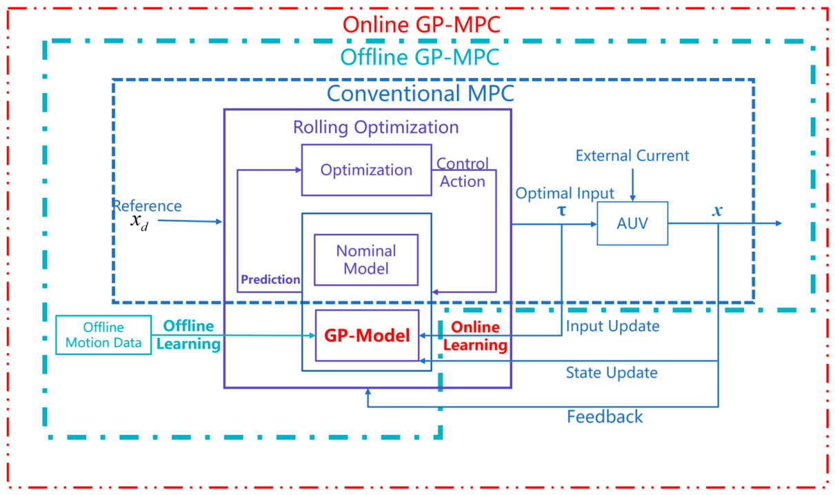
Compared with existing learning-based MPC studies, the proposed method emphasizes a lightweight residual-learning structure for real-time AUV control. The offline GP-MPC compensates for model mismatch using pre-collected residual data, while the online GP-MPC further updates the residual model using recent closed-loop data. This design allows the controller to improve disturbance compensation without requiring a large neural network dataset or a fully identified hydrodynamic model.

In this paper, two Gaussian process-based model predictive control (GP-MPC) algorithms (offline and online) are proposed to address trajectory tracking tasks for autonomous underwater vehicles (AUVs). The main objectives include building a numerical AUV model that uses Gaussian process regression to correct modeling errors, incorporating external disturbances and initial errors into a predictive control framework, and validating the approach through both simulation and real-time experiments on various trajectories. Simulation and experimental results consistently validate the robust performance of the proposed GP-MPC, even in the presence of significant initial offsets and substantial external disturbances.

Essentially, the purpose of the proposed algorithms is to combine Gaussian process regression with a model predictive control framework in order to achieve robust and accurate motion control. By leveraging real-time motion data (in the online case), the predictive model is refined to deal with uncertain factors such as ocean currents. Compared with existing controllers, the GP-MPC shows a faster transient response and improved adaptability when encountering sudden changes in the reference trajectory or significant initial errors. This ability of GP-MPC to converge within just a few seconds further highlights its rapid adjustment capabilities. Firstly, the simulation dynamics model and the nominal AUV model are described. Secondly, a novel method that utilizes GPR to augment the nominal AUV model is presented. Subsequently, a simulation platform is developed to evaluate the tracking performance of different control algorithms. Finally, the effectiveness of the proposed GP-MPC controller is validated through real-time experiments on an open-frame AUV in a pool, which involve various trajectory tracking tasks. The main contributions of this work are summarized as follows:

(1)

A GP-enhanced predictive model is developed for AUV trajectory tracking by learning the residual dynamics between a simplified nominal model and the actual/simulated vehicle response. The method is designed to operate with a small training dataset, which is important for real-time MPC implementation.

(2)

Both offline and online GP-MPC schemes are formulated. The offline GP-MPC compensates for model mismatch using pre-collected data, while the online GP-MPC further updates the residual model using a sliding window of real-time data to improve disturbance compensation.

(3)

The proposed controllers are systematically evaluated in numerical simulations under circular, L-shaped, and lemniscate trajectories, including different velocity profiles, current disturbances, and initial tracking errors.

(4)

Real-time pool experiments are conducted on an open-frame AUV to validate the practical feasibility of the GP-corrected MPC framework in surface three-DOF trajectory tracking. The experimental validation is limited to the offline GP-MPC because of the current optical tracking and real-time computing constraints, which are now explicitly discussed as limitations.

2. Numerical Model

2.1. Modeling of AUVs

In order to describe the kinematic model of an AUV, the world coordinate frame (I) and the body coordinate frame of the AUV (B) are defined, as shown in Figure 1. The attitude and position vector of the AUVs in the world coordinate frame $I$ can be expressed as $\mathit{\eta }={\left[{\mathit{\eta }}_1^{\mathrm{T}},{\mathit{\eta }}_2^{\mathrm{T}}\right]}^{\mathrm{T}}\in {\mathbb{R}}^6$, where ${\mathit{\eta }}_1={\left[x,y,z\right]}^{\mathrm{T}}$ is the position vector, and ${\eta }_2={\left[\varphi ,\theta ,\psi \right]}^{\mathrm{T}}$ is the orientation vector. The velocity and angular velocity vector of the AUVs in the body coordinate frame $V$ can be expressed as $\mathit{\nu }={\left[{\nu }_1^{\mathrm{T}},{\nu }_2^{\mathrm{T}}\right]}^{\mathrm{T}}\in {\mathbb{R}}^6$, where ${\mathit{\nu }}_1={\left[u,v,w\right]}^{\mathrm{T}}$ is the velocity vector, and ${\mathit{\nu }}_2={\left[p,q,r\right]}^{\mathrm{T}}$ is the angular velocity vector.

In marine craft modeling, the North-East-Down (NED) frame is commonly adopted following the SNAME/Fossen convention. In this study, however, an ENU-type laboratory inertial frame is used because the optical motion capture system and the ROS2-based experimental interface provide position feedback in the laboratory coordinate convention. The AUV is treated as a rigid body with six degrees of freedom in an inertial frame. The model of the AUV can be described as follows [39]:

$$\left\{\begin{array}{r}\dot{\mathit{\eta }}=\mathit{J}\left(\mathit{\eta }\right)\\ {\mathit{\tau }}_c+\mathit{T}\mathit{\tau }=M\dot{\mathit{\nu }}+C\left(\mathit{\nu }\right)\mathit{\nu }+D\left(\mathit{\nu }\right)\mathit{\nu }+g\left(\mathit{\eta }\right)\end{array}\right.,$$

(1)

where $\mathit{J}\left(\mathit{\eta }\right)$ is the rotation transformation function from the body coordinate system $B$ to the world inertial coordinate system $I$; $\mathit{M}\in {\mathbb{R}}^{6\times 6}$ is the inertia matrix; $\mathit{C}\left(\mathit{\nu }\right)\in {\mathbb{R}}^{6\times 6}$ is the Coriolis matrix; $\mathit{D}\left(\mathit{\nu }\right)\in {\mathbb{R}}^{6\times 6}$ is the damping matrix; $\mathit{g}\left(\mathit{\eta }\right)\in {\mathbb{R}}^6$ is the restoring force (the gravity and buoyancy effects); ${\mathit{\tau }}_c={\left[X_c,Y_c,Z_c,\mathrm{0,0},0\right]}^{\mathrm{T}}\in {\mathbb{R}}^6$ is the external current disturbance force; $\mathit{\tau }={\left[F_1\dots F_N\right]}^{\mathrm{T}}\in {\mathbb{R}}^N$ is the thrust vector generated by the underwater propellers; $N$ is the number of propellers; $\mathit{T}$ is the thrust allocation matrix, which depends on the position and orientation of each propeller.

In order to reduce the complexity of the model, the following assumptions are given:

(1)

The center of gravity of the AUV is chosen as the origin $O_b$ of the body coordinate system $B$. The projection of the AUV’s buoyancy center on XOY coincides with the origin. The gravity and buoyancy forces of the AUV are equal;

(2)

The mass distribution of the AUV is symmetric about the $XOZ$ and $YOZ$ planes in the body coordinate frame;

(3)

The high-order damping is ignored;

(4)

The AUV is equipped with six propellers, and the forward and reverse OARS are utilized to counteract the anti-torsion torque. The propellers are positioned in the $XOY$ plane of the body coordinate, which are symmetric with respect to the X-axis and Y-axis. The specific distribution is shown in Figure 2.

In this paper, the external current disturbance is assumed to be a bounded irrotational ocean current in the world coordinate frame. The thrust vectors can be described as:

$$\mathit{\tau }={\left[F_1,F_2,F_3,F_4,F_5,F_6\right]}^{\mathrm{T}}{\mathit{\tau }}_c={\left[X_c,Y_c,Z_c\right]}^{\mathrm{T}},$$

(2)

where $\mathit{\tau }\in {\mathbb{R}}^6$ is the thrust vector of the AUV propellers.

Based on the above assumptions, it can be assumed that the AUV has a restoring force to adjust the roll and pitch angles. Thus, the angle $\left(\varphi ,\theta \right)$ and angular velocity $\left(p,q\right)$ are considered equal to zero. The system state vector can be defined as:

$$\mathit{x}={\left[{\eta }^{\mathrm{T}},v^{\mathrm{T}}\right]}^{\mathrm{T}}\mathit{\eta }={\left[x,y,z,\psi \right]}^{\mathrm{T}}\mathit{\nu }={\left[u,v,w,r\right]}^{\mathrm{T}},$$

(3)

The simplified dynamics model of the AUV can be described as follows:

$$\dot{\mathit{x}}=f_1\left(\mathit{x}\right)+{\mathit{T}}_A\mathit{\tau }+{\mathit{T}}_B{\mathit{\tau }}_c,$$

(4)

$$f_1(\mathit{x})=\left[\begin{array}{l}u\mathrm{c}\mathrm{o}\mathrm{s}(\psi )-v\mathrm{s}\mathrm{i}\mathrm{n}(\psi )\\ v\mathrm{c}\mathrm{o}\mathrm{s}(\psi )+u\mathrm{s}\mathrm{i}\mathrm{n}(\psi )\\ w\\ r\\ {\displaystyle \frac{1}{m_{11}}}(m_{22}vr+X_{u}u+x_{u|u|}|u|u)\\ {\displaystyle \frac{1}{m_{22}}}(-m_{11}ur+Y_{v}v+Y_{v|v|}|v|v)\\ {\displaystyle \frac{1}{m_{33}}}(Z_{w}w+Z_{w|w|}|w|w)\\ {\displaystyle \frac{1}{m_{44}}}((m_{11}-m_{22})uv+N_{r}r+N_{r|r|}|r|r)\end{array}\right],$$

(5)

$${\mathit{T}}_A=\left[\begin{array}{llllll}0& 0& 0& 0& 0& 0\\ 0& 0& 0& 0& 0& 0\\ 0& 0& 0& 0& 0& 0\\ 0& 0& 0& 0& 0& 0\\ {\displaystyle \frac{\mathrm{s}\mathrm{i}\mathrm{n}\left({\theta }_T\right)}{m_{11}}}& {\displaystyle \frac{\mathrm{s}\mathrm{i}\mathrm{n}\left({\theta }_T\right)}{m_{11}}}& -{\displaystyle \frac{\mathrm{s}\mathrm{i}\mathrm{n}\left({\theta }_T\right)}{m_{11}}}& -{\displaystyle \frac{\mathrm{s}\mathrm{i}\mathrm{n}\left({\theta }_T\right)}{m_{11}}}& 0& 0\\ {\displaystyle \frac{\mathrm{c}\mathrm{o}\mathrm{s}\left({\theta }_T\right)}{m_{22}}}& -{\displaystyle \frac{\mathrm{c}\mathrm{o}\mathrm{s}\left({\theta }_T\right)}{m_{22}}}& {\displaystyle \frac{\mathrm{c}\mathrm{o}\mathrm{s}\left({\theta }_T\right)}{m_{22}}}& -{\displaystyle \frac{\mathrm{c}\mathrm{o}\mathrm{s}\left({\theta }_T\right)}{m_{22}}}& 0& 0\\ 0& 0& 0& 0& {\displaystyle \frac{1}{m_{33}}}& {\displaystyle \frac{1}{m_{33}}}\\ {\displaystyle \frac{d}{m_{44}}}& -{\displaystyle \frac{d}{m_{44}}}& -{\displaystyle \frac{d}{m_{44}}}& {\displaystyle \frac{d}{m_{44}}}& 0& 0\end{array}\right],$$

$${\mathit{T}}_B=\left[\begin{array}{lll}0& 0& 0\\ 0& 0& 0\\ 0& 0& 0\\ 0& 0& 0\\ {\displaystyle \frac{1}{m_{11}}}& 0& 0\\ 0& {\displaystyle \frac{1}{m_{22}}}& 0\\ 0& 0& {\displaystyle \frac{1}{m_{33}}}\\ 0& 0& 0\end{array}\right],$$

where $\mathit{x}\in {\mathbb{R}}^8$ and $\tau \in {\mathbb{R}}^6$ are the state and control variables of the system, respectively; $m_{ii}\left(i=1\dots 4\right)$ are the mass terms, including the mass of the AUV body, and the added mass; $X_u,Y_v,Z_w,N_r$ are the negative linear damping coefficients; $X_{u\left|u\right|},Y_{v\left|v\right|},Z_{w\left|w\right|},N_{r\left|r\right|}$ denote the negative quadratic damping coefficients, respectively; ${\tau }_c$ is the external disturbance, which is modeled as a time-varying force acting on the AUV body; ${\theta }_{\mathrm{T}}$ is defined as the angle between the propeller and the Y-axis; and $d$ is defined as the moment arm of a propeller to the origin of the body coordinate frame.

2.2. Problem Description

The trajectory tracking control of the AUV needs an accurate dynamics model. There are two difficulties in establishing the dynamics model of an AUV:

• The dynamics model is a complex MIMO system with multiple hydrodynamic coefficients, which require computational fluid dynamics (CFD) simulation or towed tank experiments to determine. However, CFD simulation often suffers from the problem of inaccurate coefficients, and towed tank experiments often require expensive experimental equipment.
• External current disturbances are difficult to measure.

To solve the above-mentioned problems, a data-driven method is proposed to enhance modeling accuracy and compensate for external disturbances. The dynamics model of an AUV is decomposed into two parts: nominal dynamics and residual dynamics. The nominal dynamics are simplified dynamics derived from the AUV dynamics model. The residual dynamics capture the residual error between the nominal and the real dynamics. The model of the AUV can be written as:

$$\dot{\mathit{x}}=f_t\left(\mathit{x},\mathit{\tau }\right)=\left[\begin{array}{l}{f}_k\left(\mathit{v}\right)\\ f_{d\_n}(\mathit{v},\mathit{\tau })\end{array}\right]+\left[\begin{array}{l}0\\ f_{d\_e}(\mathit{v},\mathit{\tau })+f_{dis}\left({\mathit{w}}_t\right)\end{array}\right],$$

(6)

where $f_k\left(v\right)$ denotes the standard kinematic equation; $f_{d\_n}(v,\tau )$ denotes the nominal dynamics obtained by the simplified analysis of the AUV dynamics; $f_{d\_e}(v,\tau )$ represents the residual error between the nominal dynamics and the real dynamics; and $f_{dis}\left(w_t\right)$ denotes the external disturbance factors, mainly the external current disturbance.

Neglecting the hydrodynamic part, the nominal dynamics model is expressed as:

$$f_{d\_n}\left(v,\tau \right)=\left[\begin{array}{l}{\displaystyle \frac{1}{m}}\left(F_1\mathrm{s}\mathrm{i}\mathrm{n}\right({\theta }_T)+F_2\mathrm{s}\mathrm{i}\mathrm{n}({\theta }_T)-F_3\mathrm{s}\mathrm{i}\mathrm{n}({\theta }_T)-F_4\mathrm{s}\mathrm{i}\mathrm{n}({\theta }_T\left)\right)\\ {\displaystyle \frac{1}{m}}\left(F_1\mathrm{c}\mathrm{o}\mathrm{s}\right({\theta }_T)-F_2\mathrm{c}\mathrm{o}\mathrm{s}({\theta }_T)+F_3\mathrm{c}\mathrm{o}\mathrm{s}({\theta }_T)-F_4\mathrm{c}\mathrm{o}\mathrm{s}({\theta }_T\left)\right)\\ {\displaystyle \frac{1}{m}}(F_5+F_6)\\ {\displaystyle \frac{1}{I_z}}(F_{1}d-F_{2}d-F_{3}d+F_{4}d)\end{array}\right]+\left[\begin{array}{l}vr\\ -ur\\ 0\\ 0\end{array}\right],$$

(7)

where $m$ is the mass of the AUV body, and $I_z$ is the moment of inertia of the AUV in the Z-axis.

2.3. Using Gaussian Process Regression to Correct the Nominal Model

Gaussian process regression (GPR) is a non-parametric regression model [40]. A Gaussian process is a set of random variables that have a joint Gaussian distribution for any finite subset.

The training dataset can be described as follows:

$$\begin{array}{c}{\mathit{D}}_{train}=\left\{X_{train}={\left[X_{trai{n}_1},X_{trai{n}_2},\dots ,X_{trai{n}_M}\right]}^{\mathrm{T}},Y_{train}={\left[Y_{trai{n}_1},Y_{trai{n}_2},\dots ,Y_{trai{n}_M}\right]}^{\mathrm{T}}\right\},\\ {\mathit{X}}_{trai{n}_i}={\left[{\mathit{\nu }}_i^{\mathrm{T}},{\mathit{\tau }}_i^{\mathrm{T}}\right]}^{\mathrm{T}}\in {\mathbb{R}}^{10}{\mathit{Y}}_{trai{n}_i}={\dot{\mathit{\nu }}}_{erro{r}_i}\in {\mathbb{R}}^{4}i\in \left[1,M\right],\\ {\dot{\mathit{\nu }}}_{error\_i}={\dot{\mathit{\nu }}}_{r\_i}-{\dot{\mathit{\nu }}}_{n\_i}\end{array}$$

(8)

where $\mathit{\nu }$ and $\mathit{\tau }$ are the control input and real speed state of the AUV; ${\dot{\mathit{\nu }}}_r$ is the real acceleration state; ${\dot{\mathit{\nu }}}_n$ is the nominal acceleration state predicted by the nominal dynamics model; ${\dot{\mathit{\nu }}}_{error}$ is the residual error between ${\dot{\nu }}_r$ and ${\dot{\nu }}_n$; and M is the data size.

GPR has multidimensional inputs and a one-dimensional output. Each dimension of the output is independent. For the $d-th$ dimension output, the mean function is considered as zero. The squared exponential (SE) kernel function is selected as the covariance function [40]:

$${\mathit{k}}_d\left(\mathit{x},{\mathit{x}}^{\prime }\right)={\mathit{\delta }}_f\mathrm{e}\mathrm{x}\mathrm{p}\left(-{\displaystyle \frac{1}{2}}{\left(\mathit{x}-{\mathit{x}}^{\prime }\right)}^{\mathrm{T}}\mathit{L}\left(\mathit{x}-{\mathit{x}}^{\prime }\right)\right),$$

(9)

where ${\mathsf{\delta }}_f$ is the variance of the data; $\mathit{L}\in {\mathbb{R}}^{10\times 10}$ is a positive diagonal matrix; and ${\mathsf{\delta }}_f, \mathit{L}$ are hyperparameters that need to be optimized by the training data.

The SE kernel is selected in this study because the residual dynamics to be learned are expected to vary smoothly with respect to the velocity and thrust inputs within the bounded operating range of the AUV. The residual term represents the difference between the nominal model and the actual/simulated response, rather than discontinuous switching dynamics. Therefore, a smooth covariance function is suitable for describing the correlation between nearby input samples. The SE kernel is also one of the most widely used covariance functions in Gaussian process regression and has been commonly adopted in GP-based dynamics learning and GP-MPC studies due to its smoothness assumption, universal approximation property, and computational simplicity.

In this work, the automatic relevance determination form of the SE kernel is used, in which different input dimensions have different length-scale hyperparameters. This allows the GP model to assign different relevance to velocity and thrust components when learning the residual dynamics. It should be noted that the present study does not claim that the SE kernel is globally optimal for all underwater conditions. For more complex real-sea environments with non-smooth, non-stationary, or depth-dependent hydrodynamic behavior, alternative kernels such as Matérn kernels or composite kernels may be more appropriate. A systematic comparison of different kernel functions will be investigated in future work.

Based on the definition of GPR, the prior distribution of the $d-th$ dimension GPR output can be given as:

$$\begin{array}{l}{\mathit{Y}}_d=\mathcal{N}\left(\mathbf{0},{\mathit{K}}_{X_{train},X_{train}}^d\right)\\ {\left[{\mathit{K}}_{X_{train},X_{train}}^d\right]}_{ij}={\mathit{k}}_d\left({\mathit{x}}_{train\_i},{\mathit{x}}_{train\_j}\right)\end{array},$$

(10)

$${\mathit{Y}}_d\in {\mathbb{R}}^M{\mathit{K}}_{X_{train},X_{train}}^d\in {\mathbb{R}}^{M\times M},$$

where ${\mathit{K}}_{X_{train},X_{train}}^d$ is the covariance matrix obtained by the squared exponential kernel function.

For a set of input $x_{tes,t}$, the prior distribution based on GPR can be expressed as:

$$\left[\begin{array}{l}{\mathit{y}}_{test,d}\\ {\mathit{Y}}_d\end{array}\right]=\mathcal{N}\left(\left[\begin{array}{l}\mathbf{0}\\ \mathbf{0}\end{array}\right],\left[\begin{array}{ll}{\mathit{K}}_{x_{test},x_{test}}^d& {\mathit{K}}_{x_{test},X_{train}}^d\\ {\mathit{K}}_{X_{train},x_{test}}^d& {\mathit{K}}_{X_{train},X_{train}}^d+\mathit{I}{\mathit{\delta }}_d^2\end{array}\right]\right),$$

(11)

$$\begin{array}{l}{\mathit{K}}_{x_{test},x_{test}}^d={\mathit{k}}_d\left({\mathit{x}}_{test},{\mathit{x}}_{test}\right)\\ {\mathit{K}}_{X_{train},x_{test}}^d={\mathit{k}}_d\left({\mathit{X}}_{train},{\mathit{x}}_{test}\right)\\ {\mathit{K}}_{x_{test},X_{train}}^d={\left({\mathit{K}}_{X_{train},x_{test}}^d\right)}^T\end{array},$$

where ${\mathsf{\delta }}_d$ is the noise variance.

Therefore, the conditional distribution of the $d-th$ dimension output can be expressed as:

$$\begin{array}{c}{\mathit{y}}_{test,d}~\mathcal{N}\left({\mathit{\mu }}_{test},{\mathsf{\Sigma }}_{test}\right)\\ {\mathit{\mu }}_{test}={\mathit{K}}_{x_{test},X_{train}}^d{\left({\mathit{K}}_{X_{train},X_{train}}^d+\mathit{I}{\delta }_d^2\right)}^{-1}{\mathit{Y}}_d\\ {\mathsf{\Sigma }}_{\mathit{t}\mathit{e}\mathit{s}\mathit{t}}={\mathit{K}}_{x_{test},x_{test}}^d-{\mathit{K}}_{x_{test},X_{train}}^d{\left[{\mathit{K}}_{X_{train},X_{train}}^d\right]}^{-1}{\mathit{K}}_{X_{train},x_{test}}^d\end{array},$$

(12)

For a new set of inputs ${\mathit{X}}_{test}={\left[{\mathit{\nu }}_{test}^{\mathrm{T}},{\mathit{\tau }}_{test}^{\mathrm{T}}\right]}^{\mathrm{T}}$, the fit equation based on GPR can be written as:

$$\begin{array}{l}{\mathit{Y}}_{test}=f_{gp}\left({\mathit{\nu }}_{test},{\mathit{\tau }}_{test}\right)\\ {\mathit{Y}}_{test}=\left[{\mathit{Y}}_{test,1},{\mathit{Y}}_{test,2},{\mathit{Y}}_{test,3},{\mathit{Y}}_{test,4}\right]\end{array},$$

(13)

The mean of the conditional distribution is selected as the prediction. Thus, the fitting equation for the output in the $d-th$ dimension ($d\in \left[\mathrm{1,4}\right]$) can be specified:

$$\begin{array}{ll}{\mathit{Y}}_{test,d}& ={\mathit{K}}_{x_{test},X_{train}}^d{\left({\mathit{K}}_{X_{train},X_{train}}^d+\mathit{I}{\mathit{\delta }}_d^2\right)}^{-1}{\mathit{Y}}_d\end{array},$$

(14)

2.4. Data Collection and Hyperparameter Training

The performance of GPR-based equation fitting is significantly influenced by the quality of the training dataset. Thus, the data points need a reasonable distribution to reflect the residual errors.

The maximum forward and reverse speeds of each axis of the AUV and the maximum forward and reverse thrusts of the propeller are formulated as follows:

$${\mathit{\nu }}_{min}\le \mathit{\nu }\le {\mathit{\nu }}_{max}{\mathit{\tau }}_{min}\le \mathit{\tau }\le {\mathit{\tau }}_{max},$$

(15)

The Latin hypercube sampling (LHS) method [41] is employed to select the training data points, which ensures an even distribution in each input dimension. The number of training data points is $M$. For the output of the $d-th$ dimension GPR, the hyperparameters are ${\mathit{\theta }}_{hyper}=\{\mathit{L},{\mathsf{\delta }}_f,{\mathsf{\delta }}_d\}$. Based on the Bayes rule [40], the posterior distribution can be expressed as:

$$p({\mathit{\theta }}_{hyper}\mid {\mathit{Y}}_d,{\mathit{X}}_{train})={\displaystyle \frac{p({\mathit{Y}}_d\mid {\mathit{X}}_{train},{\mathit{\theta }}_{hyper})p\left({\mathit{\theta }}_{hyper}\right)}{p({\mathit{Y}}_d\mid {\mathit{X}}_{train})}},$$

(16)

The optimal hyperparameter ${\mathit{\theta }}^{*}$ based on the maximum likelihood estimation (MLE) and the log marginal likelihood can be written as [40]:

$$\begin{array}{l}{\mathit{\theta }}^{\mathrm{*}}=\underset{\mathit{\theta }}{\mathrm{a}\mathrm{r}\mathrm{g}\mathrm{m}\mathrm{a}\mathrm{x}}\mathrm{l}\mathrm{o}\mathrm{g}\left(p({\mathit{Y}}_d\mid {\mathit{X}}_{train},{\mathit{\theta }}_{hyper})\right)\\ =\underset{\mathit{\theta }}{\mathrm{a}\mathrm{r}\mathrm{g}\mathrm{m}\mathrm{a}\mathrm{x}}\left[-{\displaystyle \frac{1}{2}}{\mathit{Y}}_d^T{\left[{\mathit{K}}_{X_{train},X_{train}}^d\right]}^{-1}{\mathit{Y}}_d-{\displaystyle \frac{1}{2}}\mathrm{l}\mathrm{o}\mathrm{g}|{\mathit{K}}_{X_{train},X_{train}}^d|\right]\end{array},$$

(17)

2.5. MPC for the Trajectory Tracking Control of AUVs

The desired 3D trajectory is a time-varying function of four position and four velocity degrees of freedom (${\mathit{\eta }}_d,{\mathit{\nu }}_d\in R^4$). The function can be expressed as follows:

$$\left\{\begin{array}{l}{x}_d=f_x\left(t\right)\\ y_d=f_y\left(t\right)\\ z_d=f_z\left(t\right)\\ {\psi }_d=f_{\psi }\left(t\right)\\ u_d=f_u\left(t\right)\\ v_d=f_v\left(t\right)\\ w_d=f_w\left(t\right)\\ r_d=f_r\left(t\right)\end{array}\right.,$$

(18)

where ${\mathit{\eta }}_d={\left[x_d,y_d,z_d,{\psi }_d\right]}^T$ is the position state, and ${\mathsf{\nu }}_d={\left[u_d,v_d,w_d,r_d\right]}^T$ is the velocity state.

The desired path is expressed in the body coordinate system $B$, and the desired velocity is obtained by differentiation.

The dynamics model is established by using the fitting equation of GPR:

$$\dot{\mathit{x}}=f_{cor}(\mathit{x},\mathit{\tau })=\left[\begin{array}{l}{f}_k\left(\mathit{v}\right)\\ f_{d\_n}(\mathit{v},\mathit{\tau })\end{array}\right]+\left[\begin{array}{l}0\\ f_{gp}(\mathit{v},\mathit{\tau })\end{array}\right],$$

(19)

The differential equation is discretized by the fourth-order Runge–Kutta method [42]:

$${\mathit{x}}_{k+1}=f_{Rk4}\left({\mathit{x}}_k,{\mathit{\tau }}_k,dt\right),$$

(20)

where $dt$ is the discrete time increment, ${\mathit{x}}_k$ and ${\mathit{\tau }}_k$ are the current state and input of the AUV, and ${\mathit{x}}_{k+1}$ is the state at the next time step.

The prediction step and control step are $N$. The desired state and the time steps are obtained from Equation (18), given the current time $t$, the discrete time interval $dt$, and the prediction step $N$. The predicted state ${\mathit{x}}_k\left(k\in \left[1,N\right]\right)$ in the $N$ time steps is obtained from Equation (20), given the current state ${\mathit{x}}_0$ and the control input ${\mathsf{\tau }}_k\left(k\in \left[0,N-1\right]\right)$ in the $N$ time intervals. The quadratic cost function is defined as follows:

$$\begin{array}{c}J\left({\mathit{x}}_0,\mathit{\tau }\right)={\mathit{x}}_{e_N}^{\mathrm{\top }}{\mathit{Q}}_{end}{\mathit{x}}_{e_N}+{\displaystyle \sum _{k=0}^{N-1}}{\mathit{x}}_{e_k}^{\mathrm{\top }}\mathit{Q}{\mathit{x}}_{e_k}+{\mathit{\tau }}_k^{\mathrm{\top }}\mathit{R}{\mathit{\tau }}_k\\ \{{\mathit{x}}_{e_0},\dots {\mathit{x}}_{e_N}\}=\{{\mathit{x}}_0-{\mathit{x}}_{d_0},\dots ,{\mathit{x}}_N-{\mathit{x}}_{d_N}\}\end{array},$$

(21)

where $\mathit{Q}$, $\mathit{R}$, and ${\mathit{Q}}_{end}$ denote the positive diagonal matrices of state penalty, control penalty, and terminal state penalty, respectively; $\mathit{\tau }=\left[{\mathit{\tau }}_0,{\mathit{\tau }}_1,\dots ,{\mathit{\tau }}_{N-1}\right]$ is the set of control inputs.

The essence of the MPC controller is to solve an optimal control problem (OCP) and obtain the optimal control output at the present time. The OCP is formulated as follows:

$$\underset{\tau }{\mathrm{m}\mathrm{i}\mathrm{n}}{\mathit{x}}_{e_N}^{\mathrm{\top }}{\mathit{Q}}_{end}{\mathit{x}}_{e_N}+{\displaystyle \sum _{k=0}^{N-1}}{\mathit{x}}_{e_k}^{\mathrm{\top }}\mathit{Q}{\mathit{x}}_{e_k}+{\mathit{\tau }}_k^{\mathrm{\top }}\mathit{R}{\mathit{\tau }}_k,$$

(22)

$$\begin{array}{c}\begin{array}{l}\mathrm{s}.\mathrm{t}.{\mathit{x}}_{k+1}=f_{RK4}\left({\mathit{x}}_k,{\mathit{\tau }}_k,dt\right)\\ \left\{{\mathit{x}}_{e_0},\dots {\mathit{x}}_{e_N}\right\}=\left\{{\mathit{x}}_0-{\mathit{x}}_{d_0},\dots ,{\mathit{x}}_N-{\mathit{x}}_{d_N}\right\}\end{array}\\ \begin{array}{c}{\mathit{\tau }}_{min}\le {\mathit{\tau }}_k\le {\mathit{\tau }}_{max}\\ {\mathit{x}}_{min}\le {\mathit{x}}_k\le {\mathit{x}}_{max}\\ k\in \left[0,N-1\right]\end{array}\end{array}$$

where $t$ is the current time, ${\mathit{x}}_0$ is the initial state, $\{{\mathit{x}}_{min},{\mathit{x}}_{max}\}$ is the state constraints, and $\{{\mathit{\tau }}_{min},{\mathit{\tau }}_{max}\}$ is the control input constraints.

The optimization solution ${\mathit{\tau }}^{*}$ is calculated for each control step, and ${\mathit{\tau }}_0$ is applied as the control input. At the next time step $t+dt$, the state is collected as the new initial state ${\mathit{x}}_0$, and the optimization problem is solved to obtain the new optimal control input ${\mathit{\tau }}_0$. The real-time trajectory tracking control of the AUV is achieved by repeating this process.

3. Simulation Setup and Controller Parameters

3.1. Simulation Platform Settings

The simulation parameters are detailed in

Table 1. Modeling parameters of the AUV.

Parameter	Value	Parameter	Value
$m\left(\mathrm{k}\mathrm{g}\right)$	$7.3$	$Iz\left(\mathrm{k}\mathrm{g}\mathrm{m}\right)$	$0.15$
$m_{11}\left(\mathrm{k}\mathrm{g}\right)$	$9.9$	$m_{33}\left(\mathrm{k}\mathrm{g}\right)$	$20.6$
$m_{22}\left(\mathrm{k}\mathrm{g}\right)$	$25.8$	$m_{44}\left(\mathrm{k}\mathrm{g}·\mathrm{m}\right)$	$0.43$
$Xu\left|u\right|\left(\mathrm{k}\mathrm{g}/\mathrm{m}\right)$	$-34.96$	$Zw\left|w\right|\left(\mathrm{k}\mathrm{g}/\mathrm{m}\right)$	$-74.23$
$Yv\left|v\right|\left(\mathrm{k}\mathrm{g}/\mathrm{m}\right)$	$-103.25$	$Nr\left|r\right|\left(\mathrm{k}\mathrm{g}\mathrm{m}\right)$	$-0.43$
$Xu\left(\mathrm{k}\mathrm{g}/\mathrm{s}\right)$	$0$	$Zw\left(\mathrm{k}\mathrm{g}/\mathrm{s}\right)$	$-0.19$
$Yv\left(\mathrm{k}\mathrm{g}/\mathrm{s}\right)$	$-0.26$	$Nr\left(\mathrm{k}\mathrm{g}\mathrm{m}/\mathrm{s}\right)$	$-4.64$
${\mathsf{\theta }}_T\left(\mathrm{r}\mathrm{a}\mathrm{d}\right)$	$\pi /4$	$d\left(\mathrm{c}\mathrm{m}\right)$	$15$

and are derived from the parameter identification results of the BlueRov2 as presented in [43]. A simulation platform based on Python 3.10 is established to validate the performance of different control algorithms. This platform is used to evaluate the trajectory tracking control performance of AUVs under unknown current disturbances. Various trajectory tracking tasks are executed at different speeds and with external disturbances. The performance differences between the proposed GP-MPC algorithm and the traditional cascade PID and MPC algorithms are compared.

The thrust from each of the AUV thrusters serves as the direct control input. The underlying controller determines the required thrust. These limits are common parameters of propellers available in the market. The operational area of the AUV is set as $20 \mathrm{m}\times 20 \mathrm{m}\times 15 \mathrm{m}$, and the four-degrees-of-freedom velocity limits of the AUV are set as:

$$\begin{array}{l}{\mathit{\nu }}_{min}=\{u_{min},v_{min},w_{min},r_{min}\}\\ =\{-2.5 \mathrm{m}/\mathrm{s},-1.5 \mathrm{m}/\mathrm{s},-1 \mathrm{m}/\mathrm{s},-{\displaystyle \frac{\pi }{2}} \mathrm{rad}/\mathrm{s}\}\\ {\mathit{\nu }}_{max}=\{u_{max},v_{max},w_{max},r_{max}\}\\ =\{2.5 \mathrm{m}/\mathrm{s},1.5 \mathrm{m}/\mathrm{s},1 \mathrm{m}/\mathrm{s},{\displaystyle \frac{\pi }{2}} \mathrm{rad}/\mathrm{s}\}\end{array},$$

(23)

3.2. Cascade PID Simulation Settings

In order to demonstrate the superiority of the proposed control algorithm, the traditional cascade PID control algorithm is also implemented in the simulation. The position loop and the speed loop of each axis are configured separately.

The input of the position loop is the error between the desired position and the actual position, and the output is the desired velocity. The input of the velocity loop is the error between the desired velocity and the current velocity, and the output is the thrust control command. In order to enhance the tracking performance of PID, its parameters are optimized for different trajectories. The flowchart of the cascade PID is shown in Figure 3.

In Figure 3, ${\mathit{\eta }}_d$ represents the desired position in real time, while $\mathit{\eta }$ refers to the position feedback from the robot. $\mathsf{\nu }$ denotes the velocity state feedback of the robot. $\mathit{\tau }$ is the output of the actuator, which is responsible for executing the control command.

3.3. MPC Setting

3.3.1. Nominal MPC Design

Due to the difficulties in constructing the predictive model, simplified dynamics models are commonly utilized to build the conventional MPC controller. The constraints of the MPC controller are the same, which are described in Equation (23). The prediction step $N$ is set to 5. To enhance the trajectory tracking performance of the AUV, the control penalty matrix is set to be as small as possible. The state penalty matrix is defined as $\mathit{Q}=diag\left(\mathrm{10,10,10,1},\mathrm{0.1,0.1,0.1,0.1}\right),$ and the control penalty matrix is defined as $\mathit{R}=diag\left(1e^{-3},1e^{-3},1e^{-3},1e^{-3},1e^{-3},1e^{-3},1e^{-3},1e^{-3}\right)$.

The CasADi tool [44] and Interior Point Optimizer (IPOPT) solver [45] are used to build the MPC controller. In this study, the computing device is equipped with an AMD 5800H and 16G of memory.

3.3.2. Offline GP-MPC

The training dataset of the offline GP-MPC is constructed based on the simulation results. The training data points are selected by the Latin hypercube sampling method. The simulation model and the nominal model are used to obtain the residual errors. In total, 100 sets of data are selected to train the hyperparameters of GPR.

To balance prediction accuracy and computational efficiency, 100 data samples are used to train the GPR hyperparameters, while 20 representative samples are selected from the collected raw motion data as a compact support set for constructing the GP fitting equation inside the MPC prediction model. These 20 samples are not arbitrary data points but are selected to cover the bounded operating range of the AUV as evenly as possible. This compact formulation reduces the computational burden of repeated GP evaluations during MPC optimization. Therefore, the use of 20 samples is an accuracy–complexity trade-off for real-time implementation rather than a claim of unrestricted generalization.

For clarity, the term offline GP-MPC in this study refers to the controller in which the GP residual model is constructed before closed-loop execution and remains fixed during operation. The pre-collected data are used to learn the residual dynamics between the nominal model and the reference simulation/experimental response. After the GP residual fitting function is obtained, it is directly embedded into the MPC prediction model. During closed-loop control, no new samples are added to the GP dataset, and the residual fitting function is not updated online. Therefore, the offline GP-MPC mainly compensates for repeatable model mismatch within the operating range covered by the pre-collected data. The prediction horizon, cost function, and constraints are kept the same as those of the nominal MPC so that the performance improvement can be attributed to the GP-based residual compensation.

3.3.3. Online GP-MPC

In order to compensate for the external interference, the training dataset of the online GP-MPC is divided into two parts: the offline dataset and the online dataset.

The offline dataset contains fifteen groups of offline collected data, while the online dataset consists of five groups of data that need to be collected. During the operation of the AUV, the control input and motion state are sampled in each control interval. When the online dataset consists of fewer than five groups, all of the online data are retained. If the online dataset consists of five groups, the earliest online data are discarded and the latest data are updated to the online dataset. The online dataset is updated at each control interval, and the error equation is refitted with the updated online dataset.

In contrast to the offline GP-MPC, the online GP-MPC updates the residual model during closed-loop operation. The offline data provide an initial residual model before the controller starts, while the online data reflect the most recent motion response of the AUV. At each control interval, the measured state and the applied control input are used to calculate the latest residual between the nominal acceleration and the actual acceleration. This new residual sample is then added to the online dataset. When the online dataset reaches the prescribed maximum size, the oldest online sample is removed to keep the computational complexity bounded. In this way, the online GP-MPC can adapt the residual compensation term to time-varying disturbances and recent model mismatch.

Figure 4 shows the flowchart of the nominal MPC, offline GP-MPC, and online GP-MPC. In Figure 4, ${\mathit{x}}_d={{[\mathit{\eta }}_d,{\mathit{v}}_d]}^T$ represents the desired state, while $\mathit{x}={[\mathit{\eta },\mathit{v}]}^T$ indicates the feedback state provided by the robot. The variable $\mathit{\tau }$ is the actuator’s output, which is responsible for executing the control command. The three schemes are shown as nested structures, where the nominal MPC is the basic controller, the offline GP-MPC augments it with an offline-trained GP residual model, and the online GP-MPC further extends it with an online residual-learning mechanism.

In the conventional MPC framework (inner dashed blue box), the desired state ${\mathit{x}}_d$ is used as the reference input of the rolling optimization module. Based on the nominal model, the controller predicts the future state evolution over the prediction horizon and solves an optimization problem at each control interval. The optimizer then generates the control action, and the first control input $\mathit{\tau }$ is applied to the AUV. Under the influence of the applied thrust and external current disturbances, the AUV produces the actual state response $x$, which is fed back to the controller for the next optimization step. In this way, the nominal MPC achieves closed-loop trajectory tracking through repeated prediction, optimization, and feedback.

The offline GP-MPC scheme (cyan dashed box) enhances the conventional MPC by introducing a GP-based residual model. Before closed-loop operation, offline motion data are collected and used to train the GP model. This GP model learns the residual dynamics between the nominal model and the actual AUV response and is embedded into the prediction block to correct the nominal model. Therefore, compared with the nominal MPC, the offline GP-MPC can better compensate for repeatable modeling errors and improve prediction accuracy. However, during operation, the GP model remains fixed and is not updated with new data.

The online GP-MPC scheme (outer red dashed box) further improves the offline GP-MPC by adding an online learning mechanism. During closed-loop control, the measured state $\mathit{x}$ and the applied input $\mathit{\tau }$ are continuously used to update the online dataset. The latest motion information is then employed to update the GP residual model, so that the prediction model can adapt to newly observed disturbances and time-varying uncertainties. As a result, the online GP-MPC preserves the model correction capability of the offline GP-MPC while additionally improving robustness and adaptability under changing operating conditions.

4. Numerical Simulation Results

In this section, the trajectory tracking control performance of different algorithms is studied under different trajectories, velocities, and external disturbances. The circular trajectory, L-shaped steering trajectory, and lemniscate trajectory are tracked, respectively. Additionally, the trajectory tracking task with initial errors is also studied.

The three simulation trajectories are selected to evaluate different tracking characteristics of the proposed controller. The circular trajectory is used to test steady curved path tracking under continuous yaw motion and constant curvature. The L-shaped steering trajectory is used to examine the transient response of the controller under abrupt changes in yaw angle and velocity. The lemniscate trajectory introduces coupled multi-axis motion with continuously varying curvature and velocity and is therefore used to evaluate tracking performance under more complex reference motion. In addition, the disturbance cases and initial-error case are designed to further evaluate the robustness and convergence ability of different controllers under external current disturbances and nonzero initial tracking errors.

The root mean square error (RMSE) and the maximum error (ME) of position and yaw angle are used to evaluate the trajectory tracking performance of different algorithms. The specific expression can be described as follows:

$$\mathrm{R}\mathrm{M}\mathrm{S}\mathrm{E}=\sqrt{{\displaystyle \frac{1}{M}}{\displaystyle \sum _{k=1}^M}|{\mathit{e}}_k{|}^2}\mathrm{M}\mathrm{E}=\mathrm{m}\mathrm{a}\mathrm{x}\left(\left|{\mathit{e}}_k\right|\right),$$

(24)

$$\begin{array}{c}{\mathit{e}}_k^{pos}={\mathit{\eta }}_{dk}^{pos}-{\mathit{\eta }}_{tk}^{pos}{\mathit{e}}_k^{yaw}={\mathit{\eta }}_{dk}^{yaw}-{\mathit{\eta }}_{tk}^{yaw}k\in \left[1,N\right]\\ M=T/dt\end{array},$$

where ${\eta }_{dk}^{pos}$ and ${\eta }_{dk}^{yaw}$ are the position and yaw angle of the desired trajectory at the $k$ time step, respectively; ${\eta }_{tk}^{pos}$ and ${\eta }_{tk}^{yaw}$ are the position and yaw angle of the actual tracking trajectory at the $k$ time step, respectively; $T$ is the simulation running time; and $dt$ is the discrete time interval.

In all error tables, the position RMSE and ME are reported in meters (m), and the yaw angle RMSE and ME are reported in radians (rad). These standard units are used consistently for all simulation cases.

The AUV starts from the origin of the world coordinate system $I$ with a zero yaw angle. The running time is set as $T=10\mathrm{s}$, and the discrete time interval is set as $dt=0.05\mathrm{s}$. The simulation results of different trajectory tracking tasks are given below.

4.1. No Current Disturbance and No Initial Error

4.1.1. Circular Trajectory

The radius of the circular trajectory is denoted as $r$. Define the vertical velocity as $v_z$, then the circular trajectory can be obtained as follows:

$$\begin{array}{ll}{f}_x\left(t\right)=r\mathrm{s}\mathrm{i}\mathrm{n}\left({\displaystyle \frac{\pi }{5}}t\right)& f_u\left(t\right)={\displaystyle \frac{\pi }{5}}r\\ f_y\left(t\right)=r-r\mathrm{c}\mathrm{o}\mathrm{s}\left({\displaystyle \frac{\pi }{5}}t\right)& f_v\left(t\right)=0\\ f_z\left(t\right)=v_{z}t& f_{\omega }\left(t\right)=v_z\\ f_{\psi }\left(t\right)={\displaystyle \frac{\pi }{5}}t& f_r\left(t\right)={\displaystyle \frac{\pi }{5}}\end{array},$$

(25)

The AUV performs the circular trajectory tracking task with constant linear velocity and angular velocity. The trajectory tracking performance of the AUV with different control algorithms is evaluated. Three scenarios are considered:

Case 1: $r=2 \mathrm{m}{,v}_z=0.25 \mathrm{m}/\mathrm{s}$;

Case 2: $r=3\mathrm{m}{,v}_z=0.75 \mathrm{m}/\mathrm{s}$.

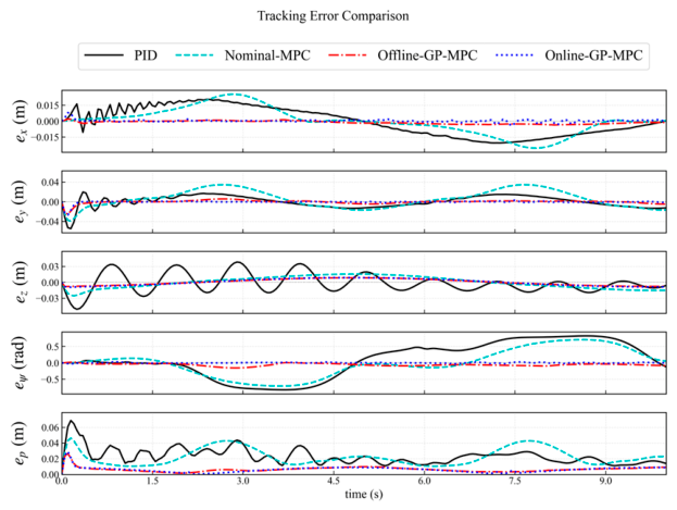
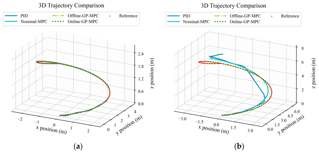
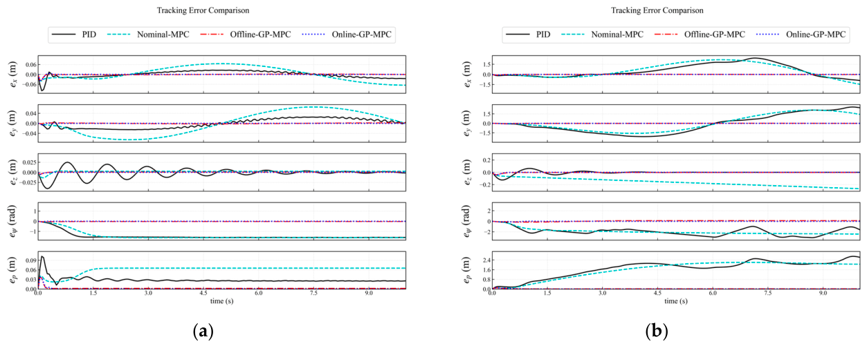
The tracking trajectories and tracking errors are shown in Figure 5 and Figure 6, respectively. The RMSE and ME are shown in

Table 2. RMSE and ME of the circular trajectory tracking task.

Simulation Case	Error		PID	Nominal MPC	Offline GP-MPC		Online GP-MPC
Case 1	Position	RMSE	0.030	0.062	0.004	↓87%	0.004	↓87%
		ME	0.103	0.065	0.037	↓43%	0.037	↓43%
	Yaw angle	RMSE	1.515	1.505	0.026	↓98%	0.005	↓99%
		ME	1.611	1.614	0.054	↓97%	0.046	↓99%
Case 2	Position	RMSE	1.827	1.757	0.022	↓98%	0.017	↓99%
		ME	2.707	2.206	0.101	↓95%	0.101	↓95%
	Yaw angle	RMSE	2.076	2.034	0.108	↓95%	0.025	↓99%
		ME	3.095	2.408	0.167	↓93%	0.123	↓95%

.

The AUV employing PID or nominal MPC algorithms can track the desired trajectories in case 1. However, as the AUV’s speed increases (case 2), the trajectories of PID or nominal MPC algorithms have obvious deviation from the desired trajectories. In contrast, the AUV utilizing the offline GP-MPC or online GP-MPC algorithms can still track the desired trajectories. Compared with PID and nominal MPC algorithms, the GP-MPC algorithms show reduced RMSE (over 90%) and ME (over 90%) in both position and yaw angle during different trajectory tracking tasks.

4.1.2. L-Shaped Steering Trajectory

The L-shaped trajectory is defined as follows: the yaw angle turns to ${90}^{\circ }$ and the $v_z$ changes from $0.25 \mathrm{m}/\mathrm{s}$ to $0.75 \mathrm{m}/\mathrm{s}$ at 5 s. The L-shaped trajectory can be described as follows:

$$\begin{array}{ll}{f}_x\left(t\right)=\left\{\begin{array}{l}1.5tt<5\\ 7.5t\ge 5\end{array}\right.& f_u\left(t\right)=1.5\\ f_y\left(t\right)=\left\{\begin{array}{l}0t<5\\ 1.5t-7.5t\ge 5\end{array}\right.& f_v\left(t\right)=0\\ f_z\left(t\right)=\left\{\begin{array}{l}0.25tt<5\\ 0.75t-2.5t\ge 5\end{array}\right.& f_{\omega }\left(t\right)=\left\{\begin{array}{l}0.25t<5\\ 0.75t\ge 5\end{array}\right.\\ f_{\psi }\left(t\right)=\left\{\begin{array}{l}0t<5\\ {\displaystyle \frac{\pi }{2}}t\ge 5\end{array}\right.& f_r\left(t\right)=0\end{array},$$

(26)

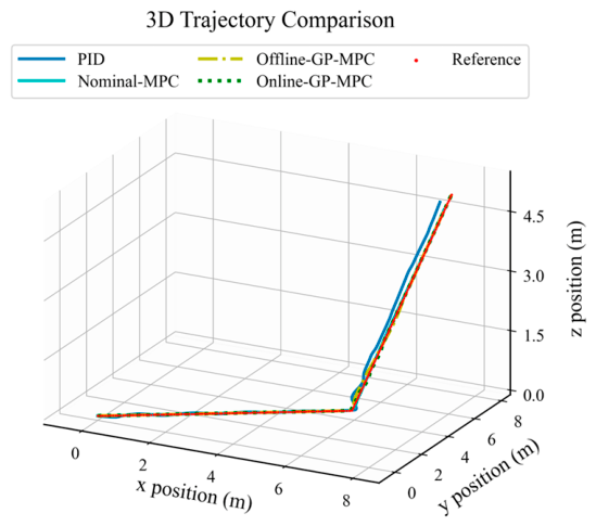
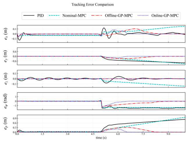
This trajectory is analyzed to evaluate the tracking performance of different algorithms under abrupt changes. The tracking trajectories and tracking errors are shown in Figure 7 and Figure 8, respectively. The RMSE and ME are shown in

Table 3. RMSE and ME of the L-shaped steering trajectory tracking task.

Error		PID	Nominal MPC	Offline GP-MPC		Online GP-MPC
Position	RMSE	0.455	0.428	0.126	↓71%	0.058	↓87%
	ME	0.836	0.975	0.312	↓63%	0.221	↓74%
Yaw angle	RMSE	1.086	1.002	0.407	↓60%	0.257	↓75%
	ME	1.690	1.459	1.309	↓11%	1.300	↓11%

.

Compared with PID and nominal MPC algorithms, the GP-MPC algorithms show reduced RMSE and ME in both position and yaw angle.

In addition, the GP-MPC algorithm can adjust the control strategy promptly to ensure that the AUV effectively follows the desired trajectory. However, the other algorithms fail to compensate for sudden changes, resulting in a large deviation of the AUV. The errors of position and yaw angle of online GP-MPC converge to the range of $1\times {10}^{-3} \mathrm{m}$ and $0.02 \mathrm{r}\mathrm{a}\mathrm{d}$ after 6.5 s. The errors of position and yaw angle of offline GP-MPC are reduced to the range of $5\times {10}^{-3} \mathrm{m}$ and $0.1 \mathrm{r}\mathrm{a}\mathrm{d}$ after 8.5 s. Therefore, the online GP-MPC algorithm demonstrates stronger robustness, smaller tracking errors, and a faster response speed, making it more suitable for various trajectory tracking tasks.

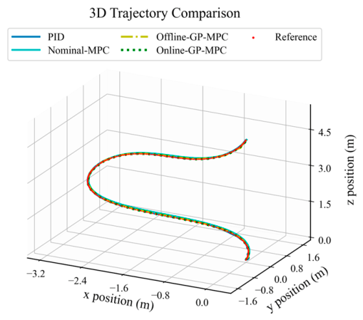
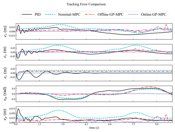
4.1.3. Lemniscate Trajectory

The lemniscate trajectory is defined as follows: the orientation is unchanged as the AUV performs the trajectory tracking tasks. The expression of this trajectory can be expressed as follows:

$$\begin{array}{ll}{f}_x\left(t\right)=1.5\mathrm{c}\mathrm{o}\mathrm{s}\left({\displaystyle \frac{\pi }{5}}t\right)-1.5& f_u\left(t\right)=-{\displaystyle \frac{3\pi }{10}}\mathrm{s}\mathrm{i}\mathrm{n}\left({\displaystyle \frac{\pi }{5}}t\right)\\ f_y\left(t\right)=\mathrm{c}\mathrm{o}\mathrm{s}\left({\displaystyle \frac{\pi }{5}}t\right)\mathrm{s}\mathrm{i}\mathrm{n}\left({\displaystyle \frac{\pi }{5}}t\right)& f_v\left(t\right)={\displaystyle \frac{\pi }{5}}\left(\mathrm{c}\mathrm{o}{\mathrm{s}}^2\left({\displaystyle \frac{\pi }{5}}t\right)-\mathrm{s}\mathrm{i}{\mathrm{n}}^2\left({\displaystyle \frac{\pi }{5}}t\right)\right)\\ f_z\left(t\right)=0.5\mathrm{s}\mathrm{i}\mathrm{n}\left({\displaystyle \frac{\pi }{5}}t\right)& f_{\omega }\left(t\right)={\displaystyle \frac{\pi }{10}}\mathrm{c}\mathrm{o}\mathrm{s}\left({\displaystyle \frac{\pi }{5}}t\right)\\ f_{\psi }\left(t\right)=0& f_r\left(t\right)=0\end{array},$$

(27)

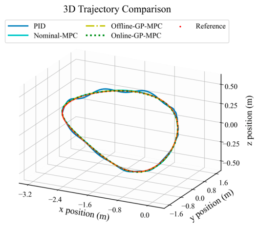
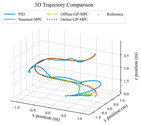
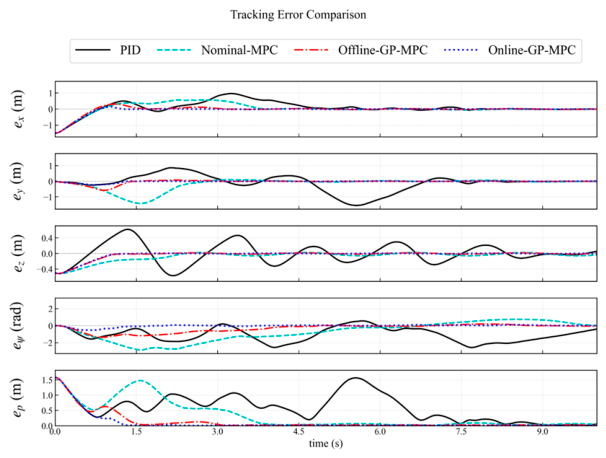
The trajectory tracking performance of different algorithms is analyzed with time-varying velocity at each axis. The tracking trajectories and tracking errors are shown in Figure 9 and Figure 10, respectively. The RMSE and ME are shown in

Table 4. RMSE and ME of the lemniscate trajectory tracking task.

Error		PID	Nominal MPC	Offline GP-MPC		Online GP-MPC
Position	RMSE	0.025	0.024	0.007	↓71%	0.007	↓71%
	ME	0.069	0.046	0.027	↓41%	0.029	↓37%
Yaw angle	RMSE	0.543	0.417	0.069	↓83%	0.011	↓97%
	ME	0.826	0.712	0.155	↓78%	0.033	↓95%

.

It can be found that the PID and nominal MPC algorithms can track the desired trajectory when the trajectory speed of the AUV changes, but they exhibit significant tracking errors (the ME of the position and yaw angle are more than 0.04 m and 0.7 rad, respectively). The offline GP-MPC and the online GP-MPC adopt data-driven methods to compensate for the modeling error, which achieves better trajectory tracking performance (over 70% reduction on the RMSE of the position and yaw angle). Furthermore, the online GP-MPC shows smaller RMSE and ME values on the yaw angle compared with the offline GP-MPC.

4.2. With Current Disturbance but No Initial Error

4.2.1. Constant Disturbance

A constant disturbance of 40 N acts on the X-axis, Y-axis, and Z-axis of the world coordinate frame $I$. The disturbance forces can be expressed as follows:

$$f_{x\_distrub}\left(t\right)=40 f_{y\_distrub}\left(t\right)=40 f_{z\_distrub}\left(t\right)=40,$$

(28)

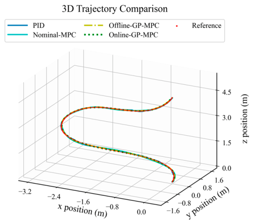
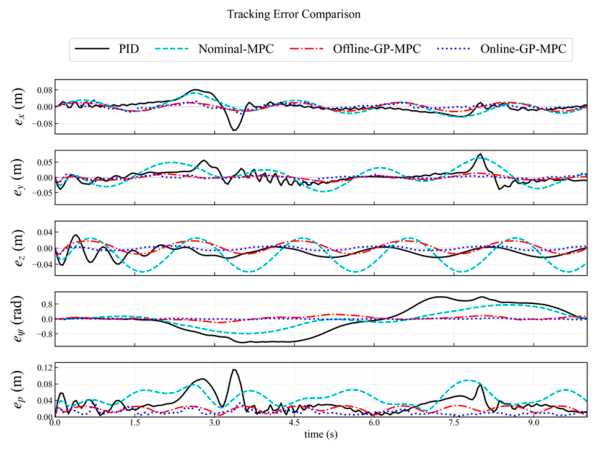
The lemniscate trajectory is defined as follows:

$$\begin{array}{ll}{f}_x\left(t\right)=1.5\mathrm{c}\mathrm{o}\mathrm{s}\left({\displaystyle \frac{\pi }{5}}t\right)-1.5& f_u\left(t\right)=-{\displaystyle \frac{3\pi }{10}}\mathrm{s}\mathrm{i}\mathrm{n}\left({\displaystyle \frac{\pi }{5}}t\right)\\ f_y\left(t\right)=\mathrm{c}\mathrm{o}\mathrm{s}\left({\displaystyle \frac{\pi }{5}}t\right)\mathrm{s}\mathrm{i}\mathrm{n}\left({\displaystyle \frac{\pi }{5}}t\right)& f_v\left(t\right)={\displaystyle \frac{\pi }{5}}\left(\mathrm{c}\mathrm{o}{\mathrm{s}}^2\left({\displaystyle \frac{\pi }{5}}t\right)-\mathrm{s}\mathrm{i}{\mathrm{n}}^2\left({\displaystyle \frac{\pi }{5}}t\right)\right)\\ f_z\left(t\right)=0.5t& f_{\omega }\left(t\right)=0.5\\ f_{\psi }\left(t\right)=0& f_r\left(t\right)=0\end{array},$$

(29)

A simulation of lemniscate trajectory tracking under constant disturbance is conducted. The simulation result and tracking errors are shown in Figure 11 and Figure 12, respectively. The RMSE and ME are shown in

Table 5. RMSE and ME of the lemniscate trajectory tracking task with constant disturbance.

Error		PID	Nominal MPC	Offline GP-MPC		Online GP-MPC
Position	RMSE	0.021	0.038	0.017	↓20%	0.008	↓62%
	ME	0.075	0.067	0.043	↓36%	0.025	↓63%
Yaw angle	RMSE	0.562	0.416	0.410	↓2%	0.011	↓97%
	ME	0.875	0.711	1.052	↑47%	0.062	↓91%

.

The tracking performance of nominal MPC and offline GP-MPC degrades under the influence of external disturbances. Due to the integrator, the PID algorithm exhibits a certain interference compensation effect, which maintains nearly unaltered tracking performance. The tracking performance of offline GP-MPC is significantly degraded. Compared with the over 70% RMSE reduction achieved without external interference, the RMSE reduction is now only 20%. Relative to PID and nominal MPC, the position tracking error of offline GP-MPC is only slightly reduced, and the yaw angle error is increased. The online GP-MPC compensates for the external interference by collecting the real-time motion data of the AUV, which achieves excellent tracking performance (the RMSE of the position and yaw angle are 0.008 m and 0.011 rad, respectively). Consequently, the RMSE and ME of the position are reduced by more than 60%, and the RMSE and ME of the yaw angle are reduced by more than 90%. The simulation results demonstrate that the online GP-MPC has strong robustness against constant external interference.

4.2.2. Time-Varying Disturbance

Considering the time-varying disturbances in the X-axis, Y-axis, and Z-axis of the world coordinate system $I$, to evaluate the disturbance rejection ability of different controllers under repeatable conditions, a bounded sinusoidal time-varying disturbance is adopted in this simulation case. Sinusoidal and bounded time-varying disturbances are commonly used as benchmark disturbances in underwater vehicle control studies because they provide reproducible disturbance conditions for controller comparison. It should be noted that this disturbance model is a simplified benchmark rather than a complete representation of real ocean current dynamics. The purpose of this case is to examine whether the online GP-MPC can update the residual model using recent closed-loop data and improve tracking performance under time-varying external forces.

The specific expression can be described as follows:

$$\begin{array}{l}{f}_{x\_distrub}\left(t\right)=75\mathrm{s}\mathrm{i}\mathrm{n}\left(t\right)\\ f_{y\_distrub}\left(t\right)=75\mathrm{c}\mathrm{o}\mathrm{s}\left(t\right)\\ f_{z\_distrub}\left(t\right)=50\mathrm{s}\mathrm{i}\mathrm{n}\left(t\right)\end{array},$$

(30)

The simulation result and tracking errors are shown in Figure 13 and Figure 14, respectively. The RMSE and ME are shown in

Table 6. RMSE and ME of the lemniscate trajectory tracking task with time-varying disturbance.

Error		PID	Nominal MPC	Offline GP-MPC		Online GP-MPC
Position	RMSE	0.037	0.051	0.020	↓46%	0.012	↓68%
	ME	0.115	0.089	0.028	↓69%	0.034	↓62%
Yaw angle	RMSE	0.760	0.426	0.100	↓77%	0.020	↓95%
	ME	1.267	0.783	0.245	↓69%	0.068	↓91%

.

The RMSE of the position and yaw angle increases to 0.037 m and 0.76 rad, which indicates that PID exhibits poor robustness to time-varying external disturbances. The nominal MPC also becomes less effective, leading to an increase in the RMSE of the position and yaw angle to 0.051 m and 0.426 rad, respectively. The offline GP-MPC shows better tracking performance compared with PID and nominal MPC. The RMSE of the position and yaw angle exhibits reductions of 46% and 77%. The online GP-MPC utilizes real-time data to enhance the predictive model and compensate for external interference. The RMSE of the position and yaw angle shows reductions of 68% and 95%, which shows strong robustness to external time-varying disturbances.

4.3. With Current Disturbance and Initial Error

The lemniscate trajectory is translated forward to the X-axis by 1.5 m and the Z-axis by 0.5 m. Thus, the trajectory can be expressed as:

$$\begin{array}{ll}{f}_x\left(t\right)=1.5\mathrm{c}\mathrm{o}\mathrm{s}\left({\displaystyle \frac{\pi }{5}}t\right)& f_u\left(t\right)=-{\displaystyle \frac{3\pi }{10}}\mathrm{s}\mathrm{i}\mathrm{n}\left({\displaystyle \frac{\pi }{5}}t\right)\\ f_y\left(t\right)=\mathrm{c}\mathrm{o}\mathrm{s}\left({\displaystyle \frac{\pi }{5}}t\right)\mathrm{s}\mathrm{i}\mathrm{n}\left({\displaystyle \frac{\pi }{5}}t\right)& f_v\left(t\right)={\displaystyle \frac{\pi }{5}}\left(\mathrm{c}\mathrm{o}{\mathrm{s}}^2\left({\displaystyle \frac{\pi }{5}}t\right)-\mathrm{s}\mathrm{i}{\mathrm{n}}^2\left({\displaystyle \frac{\pi }{5}}t\right)\right)\\ f_z\left(t\right)=0.5t+0.5& f_{\omega }\left(t\right)=0.5\\ f_{\psi }\left(t\right)=0& f_r\left(t\right)=0\end{array},$$

(31)

The external time-varying disturbance in Equation (31) is added. The lemniscate trajectory tracking task in the presence of time-varying disturbance and initial errors is simulated. The simulation result and tracking errors are shown in Figure 15 and Figure 16, respectively. The RMSE and ME are shown in

Table 7. RMSE and ME of the lemniscate trajectory tracking task with time-varying disturbance and initial error.

Error		PID	Nominal MPC	Offline GP-MPC		Online GP-MPC
Position	RMSE	0.723	0.552	0.313	↓44%	0.289	↓48%
	ME	1.581	1.581	1.581	0%	1.581	0%
Yaw angle	RMSE	1.341	1.294	0.541	↓59%	0.135	↓90%
	ME	2.556	2.831	1.362	↓47%	0.532	↓80%

.

The PID algorithm exhibits a slow response speed, which fails to track the reference trajectory by the end of the simulation. MPC-based algorithms show faster convergence, with position errors stabilizing after 5 s. The position error of nominal MPC converges to the range of 0.1 m after 4.5 s, but the yaw angle error fails to converge. The position error of the offline GP-MPC converges to the range of 0.03 m after 3 s, and the yaw angle error converges to the range of 0.2 rad after 5 s. The position error of the online GP-MPC converges to the range of 0.15 m after 1.5 s, and the yaw angle error converges to the range of 0.1 rad after 1.5 s. The simulation results show that the GP-MPC algorithms employed in this paper exhibit smaller tracking errors, stronger robustness, and faster response speeds. In the comparison of the two GP-MPC algorithms, the online GP-MPC algorithm demonstrates superior tracking performance.

4.4. Comparative Discussion of Offline and Online GP-MPC

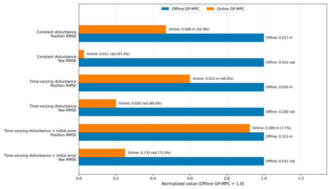
To further clarify the advantage of the online residual update, a direct comparison between offline GP-MPC and online GP-MPC is summarized in

Table 8. Performance improvement of online GP-MPC over offline GP-MPC under challenging conditions.

Case	Metric	Offline GP-MPC	Online GP-MPC	Improvement of Online Update
Constant disturbance	Position RMSE	0.017 m	0.008 m	52.9%
	Yaw RMSE	0.410 rad	0.011 rad	97.3%
Time-varying disturbance	Position RMSE	0.020 m	0.012 m	40.0%
	Yaw RMSE	0.100 rad	0.020 rad	80.0%
Time-varying disturbance + initial error	Position RMSE	0.313 m	0.289 m	7.7%
	Yaw RMSE	0.541 rad	0.135 rad	75.0%

.

Under constant current disturbance, the online GP-MPC reduces the position RMSE from 0.017 m to 0.008 m and the yaw RMSE from 0.410 rad to 0.011 rad compared with the offline GP-MPC. Under time-varying disturbance, the online update reduces the position RMSE by 40.0% and the yaw RMSE by 80.0%. When both time-varying disturbance and initial error are considered, the improvement in position RMSE is relatively moderate, but the yaw RMSE is still reduced by 75.0%. Figure 17 shows the normalized RMSE comparison between offline GP-MPC and online GP-MPC under disturbance and initial-error conditions. Each metric is normalized by the corresponding offline GP-MPC result. Under constant disturbance, the online GP-MPC reduces the position RMSE and yaw RMSE by 52.9% and 97.3%, respectively. Under time-varying disturbance, the corresponding reductions are 40.0% and 80.0%. When both time-varying disturbance and initial error are considered, the position RMSE improvement is relatively small, mainly because the initial position offset dominates the transient position error.

Nevertheless, the yaw RMSE is still reduced by 75.0%. These results demonstrate that the online residual update improves the robustness of GP-MPC, especially for yaw tracking under time-varying disturbances.

5. Real-Time Experimental Results

To validate the effectiveness and robustness of the proposed control solution, multiple experimental trials are conducted in an indoor pool. The AUV is controlled by a low-level control unit, which uses an STM32F407 microcontroller to acquire sensor data and control the thruster motors. A Jetson Xavier NX single-board computer handles high-level control modules and other functions such as vision and planning. The STM32F407 and Jetson Xavier NX communicate through a serial interface.

Table 9. Main characteristics of the AUV.

Characteristic	Value
Mass	12.5 kg
Residual Buoyancy	10 N
Dimensions	50 × 40 × 25 cm
Power	24 V–500 W
Thrusters	6 × Rovmaker 2216
Inertial Measurement Unit (IMU)	BMI088
Depth Sensor	MS5837-30BA
Attitude Sensor	WT9053
Onboard Microcontroller Unit (MCU)	STM32F407VET6
High-Level Controller	Jetson Xavier NX

details the main characteristics of the AUV used in the experiments.

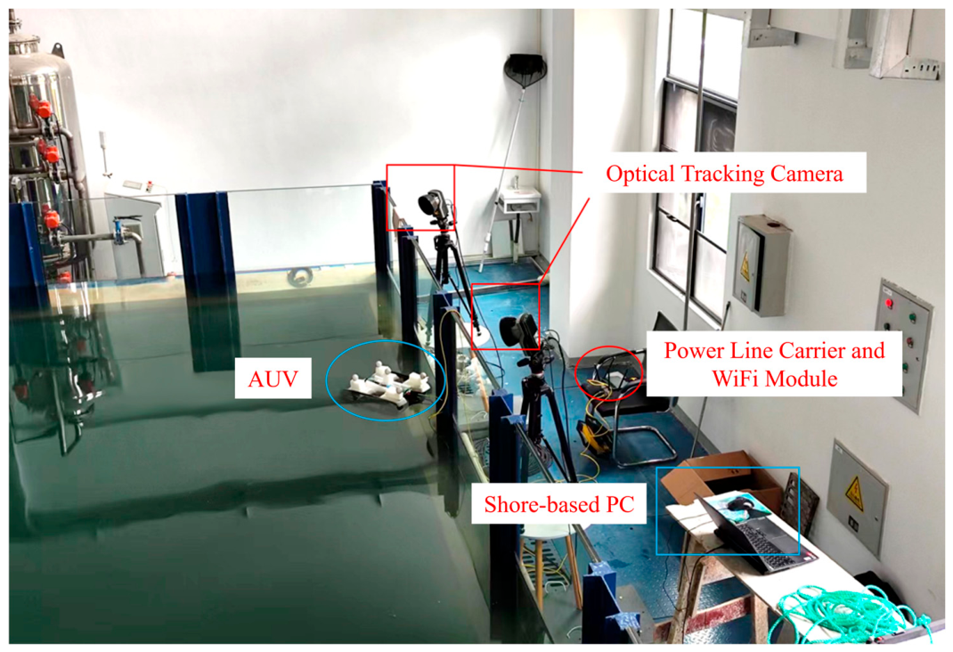
The numerical simulations and physical experiments serve different but complementary purposes in this study. The simulations are designed to systematically evaluate the controller under different trajectories, velocities, external current disturbances, and initial errors, whereas the pool experiments are mainly used to validate the real-time implementation feasibility of the proposed GP-MPC framework on the physical AUV. During the trials, the Oqus 700+ optical motion capture cameras are used to provide position and velocity feedback for the AUV when it operates on the water surface. This system can provide position feedback within a 2 m × 2 m tracking range at a frequency of 100 Hz, and the real-time state information is transmitted to the motion control system through Qualisys Track Manager software integrated with a self-developed Robot Operating System 2 (ROS2) package. Since the Oqus 700+ optical motion capture system can only track markers above the water surface, the physical experiments are limited to closed-loop motion control in three degrees of freedom on the water surface. Therefore, the experimental trajectories are scaled and simplified compared with the simulation trajectories to ensure safe and reliable operation within the available sensing range. The real experiments do not aim to reproduce all simulation cases exactly, but to verify whether the proposed controller can be implemented and executed reliably on the physical platform. The same RMSE and ME metrics are used in both simulation and experimental evaluations. The experimental setup is illustrated in Figure 18.

The optical cameras capture the trajectories of the marked spheres and send the data to a shore-based PC via Ethernet. The Qualisys Track Manager software 2023 processes this data to determine the state of the AUV and transmits it via the Transmission Control Protocol (TCP) to an Ubuntu 20 virtual machine on the PC. The ROS2 Foxy software within the virtual machine receives the AUV state information and executes the control algorithm. It then sends motor commands via power line communication to the Xavier, which drives the AUV and forms a closed-loop control system.

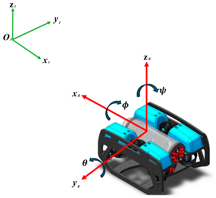
The six-DOF formulation in Equation (1) is used as the general modeling basis. Under the symmetry and hydrostatic assumptions stated in this section, roll and pitch are passively stabilized and are not included in the predictive control state. Therefore, the simulation controller is designed for a reduced four-DOF model $(x,y,z,\psi )$. In the pool experiments, the optical motion capture system can only track markers above the water surface; therefore, the depth channel is kept fixed, and the real-time closed-loop validation is restricted to surface three-DOF motion $(x,y,\psi )$. This limitation does not change the GP-MPC formulation, but it means that the experiments verify the real-time feasibility of the GP-corrected MPC framework rather than full underwater six-DOF control.

The primary objective of Gaussian process-based model predictive control is to accurately track the predefined trajectory in the presence of parametric uncertainties. To demonstrate the advantages of the proposed algorithm, a comparative analysis was conducted, which included evaluations of PID, nominal MPC, and GP-MPC.

5.1. Control Methods in Comparative Experiments

5.1.1. Cascade PID

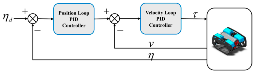
In the comparative experiments, a cascade PID controller is used as the traditional control baseline. The PID parameters are tuned through repeated closed-loop trials to obtain the best performance for each experimental task.

5.1.2. Nominal MPC

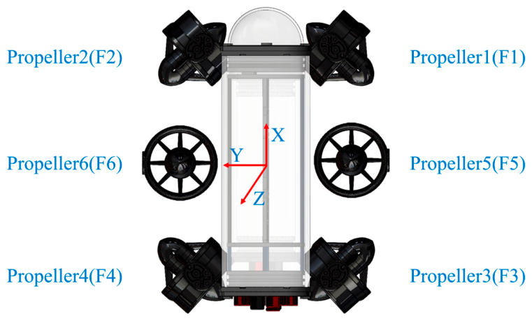
The design steps for the MPC-based horizontal position control experiment are largely consistent with those that are employed in the previous simulations. During the modeling of the AUV, depth control is ignored, and the focus is placed solely on the three degrees of freedom in horizontal motion. The nominal model, which is used as the predictive model, applies the actual specifications of the AUV for mass, moments of inertia, thruster angles, and lever arms, without accounting for hydrodynamic coefficients.

After extensive experimentation and parameter tuning, the state penalty matrix is set as $\mathit{Q}=diag\left\{\mathrm{10,10,10,0.01,0.01,0.01}\right\}$, the terminal state penalty matrix is set as ${\mathit{Q}}_{end}=diag\left\{\mathrm{30,30,30,0.03,0.03,0.03}\right\}$, and the control input penalty matrix is set as $\mathit{R}=diag\left\{\mathrm{0.001,0.001,0.001,0.001}\right\}$. Both the prediction horizon and control horizon are set to 5, with a control frequency of 10 Hz. The thrust output of the underwater thrusters is constrained between −15 N and 15 N. Multiple tests are conducted to determine the velocity limits for each degree of freedom, resulting in a limit of −1 m/s to 1 m/s for X-axis motion, −0.5 m/s to 0.5 m/s for Y-axis motion, and $-\mathsf{\pi } \mathrm{r}\mathrm{a}\mathrm{d}/\mathrm{s}$ to $\mathsf{\pi } \mathrm{r}\mathrm{a}\mathrm{d}/\mathrm{s}$ for yaw rate. The state constraints are therefore selected as $x_{\mathrm{m}\mathrm{i}\mathrm{n}}=\left[-1,-1,-100\mathsf{\pi },-1,-0.5,-\mathsf{\pi }\right]$ and $x_{\mathrm{m}\mathrm{a}\mathrm{x}}=\left[\mathrm{1,1},100\mathsf{\pi },\mathrm{1,0.5},\mathsf{\pi }\right]$.

5.1.3. GP-MPC

The primary distinction between GP-MPC and nominal MPC lies in the use of GPR to refine the robot’s motion control model. In the practical experiments, the PID algorithm and the nominal MPC algorithm are first used to drive the AUV for various tasks. In order to fit the motion control model, it is necessary to obtain the AUV’s acceleration errors. Since the optical tracking system cannot provide real-time acceleration data, the velocity error can be obtained by using the following equation:

$$a_{ek}={\displaystyle \frac{v_{k+1}-{\widehat{v}}_{k+1}}{dt}},$$

(32)

where $v_{k+1}$ represents the actual AUV velocity measured at time step $k+1$; ${\widehat{v}}_{k+1}$ denotes the AUV velocity predicted by the nominal model at time step $k+1$; and $dt$ is the time interval.

The offline GP-MPC algorithm requires the collection of AUV motion data to generate a training dataset $D_{all}$, with input and output content largely consistent with the simulation. The primary difference lies in using the approximation of acceleration error obtained from Equation (32) as the output. Additionally, since the control task involves three degrees of freedom on the water surface, the input and output dimensions have been adjusted according to the actual scenario. This dataset is then used to fit the corrected hybrid motion control model.

To ensure that the data used for GPR training is comprehensively distributed across the input space, we developed an algorithm specifically designed to select optimal training data points from the complete set of motion state data.

Due to the varying upper and lower bounds of the motion state variables across different axes, normalization of the motion data is required to prevent significant discrepancies in scale. Since each state variable and control input has distinct bounds, this paper employs the widely used min–max normalization method, which can be described as follows:

$$x_{\mathrm{s}\mathrm{c}\mathrm{a}\mathrm{l}\mathrm{e}}={\displaystyle \frac{x-x_{\mathrm{m}\mathrm{i}\mathrm{n}}}{x_{\mathrm{m}\mathrm{a}\mathrm{x}}-x_{\mathrm{m}\mathrm{i}\mathrm{n}}}},$$

(33)

where $x_{\mathrm{m}\mathrm{a}\mathrm{x}}$ and $x_{\mathrm{m}\mathrm{i}\mathrm{n}}$ represent the maximum and minimum boundaries of the data to be normalized. $x$ is the value before normalization, and $x_{\mathrm{s}\mathrm{c}\mathrm{a}\mathrm{l}\mathrm{e}}$ is the value after normalization.

To select data points, it is essential to calculate the distance between them as the selection criterion. The Euclidean distance is used for this purpose, as described below:

$$d=\left|x_1-x_2\right|,$$

(34)

where $x_1$ and $x_2$ represent data points in vector form, with the Euclidean distance defined as the magnitude of the vector obtained by subtracting one from the other.

After preprocessing the motion state data, a dataset selection algorithm is applied to filter out a well-distributed set of motion state data to form the training dataset. The specific selection method involves first iterating through all data points and calculating the Euclidean distance between each pair. A minimum distance threshold $d_{\mathrm{m}\mathrm{i}\mathrm{n}}$ is then defined between data points. The data points are iterated through again, and if the Euclidean distance between the current data point and all points in the training set is greater than $d_{\mathrm{m}\mathrm{i}\mathrm{n}}$, it is added to the training dataset. Ultimately, all data points in the selected dataset must have Euclidean distances greater than $d_{\mathrm{m}\mathrm{i}\mathrm{n}}$. The size of the dataset can be adjusted by modifying the distance threshold $d_{\mathrm{m}\mathrm{i}\mathrm{n}}$.

Considering both model accuracy and computational complexity, the final dataset size selected for hyperparameter training is 100, while the dataset size for constructing the GPR fitting equation is 20. The constraints, penalty matrices, control frequency, prediction horizon, and control horizon used in the controller design are identical to those in the nominal MPC experiment.

5.2. Scenario 1: Circular Trajectory Tracking Experiment

In this scenario, the AUV is programmed to execute a low-speed circular motion, and the desired trajectory is defined as follows:

$$\left\{\begin{array}{l}{f}_x\left(t\right)=0.7-0.5\mathrm{c}\mathrm{o}\mathrm{s}\left({\displaystyle \frac{\pi }{4}}t\right)\\ f_y\left(t\right)=-0.1-0.5\mathrm{s}\mathrm{i}\mathrm{n}\left({\displaystyle \frac{\pi }{4}}t\right)\\ f_{\psi }\left(t\right)={\displaystyle \frac{\pi }{4}}t-\pi \end{array}\right.,$$

(35)

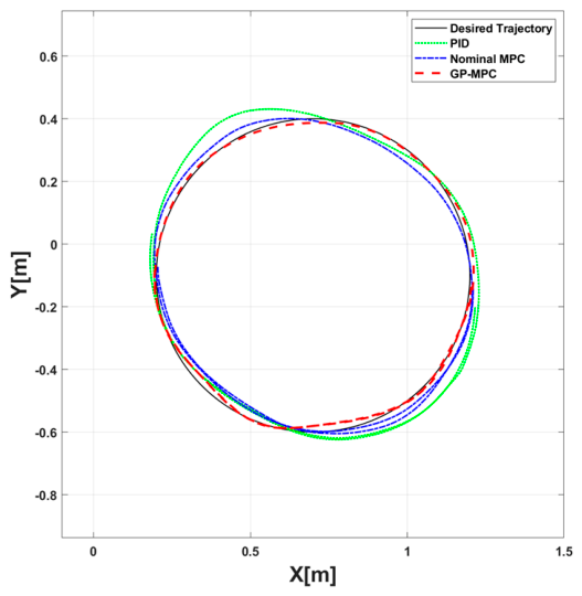
During data processing, the yaw angle is normalized to the standard $-\mathsf{\pi }$ to $\mathsf{\pi }$ range via a modulo operation. Figure 19 illustrates the tracking performance of the three controllers on a circular trajectory under conditions of parametric uncertainty.

As shown in Figure 19 and Figure 20, the MPC-based methods exhibit stable control performance overall, without significant sudden fluctuations and with relatively small deviations from the desired trajectory.

The performance comparison

Table 10. Performance of low-speed circular trajectory tracking using different methods.

Error		PID	Nominal MPC	Offline GP-MPC
X	RMSE	0.047	0.028	0.017
	ME	0.079	0.048	0.032
Y	RMSE	0.090	0.064	0.022
	ME	0.143	0.098	0.042
Yaw	RMSE	0.182	0.134	0.052
	ME	0.273	0.042	0.090

shows that nominal MPC reduces the root mean square error and maximum error for each axis by approximately 40% when compared with PID. GP-MPC, which uses a data-driven approach to compensate for model inaccuracies, further reduces the overall root mean square error and maximum error by over 60%, resulting in a trajectory that more closely follows the desired path. This demonstrates that the GP-MPC algorithm has a clear advantage in executing complex multi-degree-of-freedom tracking control tasks.

5.3. Scenario 2: Trajectory Tracking Experiment with Time-Varying Velocity

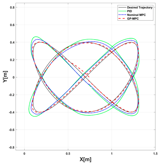
In order to analyze the tracking performance of different algorithms on a time-varying velocity trajectory, the AUV is programmed to follow a trajectory defined by a velocity function. The desired yaw angle of the AUV is set to remain constant, while the AUV tracks a relatively complex trajectory through its X-axis and Y-axis movements. The desired trajectory can be described as:

$$\left\{\begin{array}{l}{f}_x\left(t\right)=0.7-0.6\mathrm{s}\mathrm{i}\mathrm{n}\left(t\times \pi /6\right)\\ f_y\left(t\right)=0.4\mathrm{s}\mathrm{i}\mathrm{n}\left(t\times \pi /4\right)\\ f_{\psi }\left(t\right)=0\end{array}\right.,$$

(36)

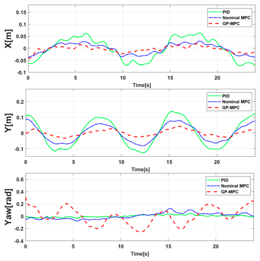
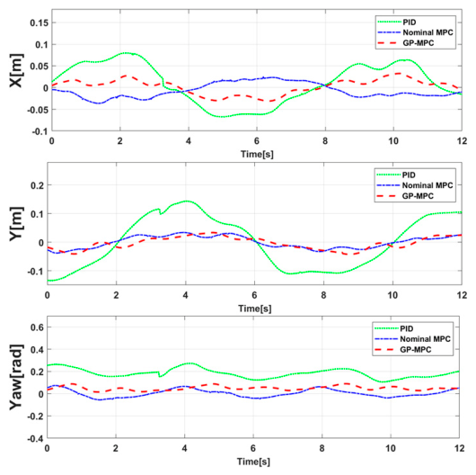
Figure 21 shows the tracking curves for the variable-speed trajectory, which are executed by different methods.

Figure 22 presents the tracking errors for each axis, which are determined by analyzing the motion data from different algorithms.

Figure 21 and Figure 22 show that the MPC-based methods have better performance in reducing position tracking errors; however, they exhibit larger yaw angle tracking errors. This is because the penalty matrix assigns a higher penalty to position errors, which causes the controller to minimize these errors. The significant resistance encountered during Y-axis translation forces the AUV to adjust its yaw angle to maintain accurate position tracking.

According to

Table 11. Performance of complex trajectory tracking using different methods.

Error		PID	Nominal MPC	Offline GP-MPC
X	RMSE	0.045	0.021	0.013
	ME	0.073	0.038	0.042
Y	RMSE	0.085	0.052	0.019
	ME	0.136	0.087	0.042
Yaw	RMSE	0.017	0.048	0.134
	ME	0.048	0.125	0.309

, nominal MPC reduces the position error by nearly 25 mm compared with the PID algorithm, although it increases the average yaw angle error by 0.03 rad, which accounts for 45% of the total position error in the PID algorithm. The actual trajectory is more closely aligned with the desired trajectory, particularly at the trajectory’s edges. It is clear that position error is generally more pronounced in trajectory tracking. When considered across all axes, the control performance provided by the proposed method is reasonable and near optimal.

Similarly, GP-MPC reduces the position error by nearly 75 mm, which represents 70% of the total position error of the PID algorithm, although it increases the average yaw angle error by 0.12 rad. The overall trajectory nearly coincides with the desired path. GP-MPC has better performance than both PID and nominal MPC in overall position tracking accuracy, which makes it the most effective algorithm for tracking errors across all axes.

6. Conclusions

In this paper, Gaussian process-based model predictive control (GP-MPC) algorithms are proposed for AUV trajectory tracking control. A Python-based simulation platform is developed to evaluate the proposed controllers under circular, L-shaped, and lemniscate trajectories, including current disturbances and initial errors. Real-time pool experiments are also conducted on an open-frame AUV to validate the feasibility of the offline GP-MPC in surface three-DOF trajectory tracking. The main conclusions are summarized as follows:

(1)

Compared with cascade PID and nominal MPC, the proposed GP-MPC algorithms achieve better tracking accuracy by learning the residual dynamics between the nominal model and the actual/simulated AUV response. In different trajectory tracking tasks, the RMSE and ME are reduced by more than 40%.

(2)

The online GP-MPC improves disturbance compensation by updating the residual model with recent closed-loop data. Compared with offline GP-MPC, the online GP-MPC reduces the yaw RMSE by 97.3%, 80.0%, and 75.0% under constant disturbance, time-varying disturbance, and time-varying disturbance with initial error, respectively. This demonstrates the advantage of online residual updating under time-varying residual dynamics.

(3)

Under abrupt trajectory changes and initial tracking errors, GP-MPC shows faster convergence and better transient response than PID and nominal MPC. The online GP-MPC further improves adaptability by incorporating recent motion data through a sliding-window update.

(4)

The real-time pool experiments demonstrate that the offline GP-MPC can improve the trajectory tracking accuracy of the physical AUV under the current surface three-DOF experimental setup.

The present study still has several limitations. The physical experiments are limited to surface three-DOF motion due to the lack of reliable underwater feedback, so they validate the real-time feasibility of the GP-corrected MPC framework rather than full underwater six-DOF control. The online GP-MPC is currently validated through numerical simulations, and its closed-loop physical validation remains to be explored in future work. Future studies will focus on underwater localization, sparse/local online GP implementation, and benchmark validation under more realistic marine disturbances.