Cross-Domain Transferability of Foliar Nitrogen Prediction in Sugarcane (Saccharum officinarum) Through the Integration of UAV and Simulated Spectral Data

Highlights

What are the main findings?

• The proposed methodological approach was crucial for the consistency of the results, demonstrating robust predictive performance for nitrogen content, with R² = 0.75 (PLSR) and 0.76 (RF) for UAV data, and R² = 0.75 (PLSR) and 0.74 (RF) for simulated data.
• Even with a reduced spectral range, the simulated data retained high predictive power, with indices such as ChlRe (R² = 0.74) and NDVI (R² = 0.71), indicating that information relevant for N estimation was preserved.

What are the implications of the main findings?

• This approach validates the use of spectral simulation as a strategy for transferring information from the hyperspectral domain to multispectral sensors without any significant loss of performance.
• The results underscore the potential for application in operational settings with limited data, enhancing the feasibility of nutritional monitoring via UAV using more generalizable models.

Abstract

Remotely Piloted Aircrafts (RPAs) equipped with multispectral sensors have emerged as promising tools for estimating foliar nitrogen content (TFN). So, this study applied a methodological approach aimed at simulating UAV multispectral data using hyperspectral leaf data obtained in a controlled environment, with the objective of evaluating its predictive potential and its transferability to field data collected by UAVs for TFN estimation. To this end, spectral bands and spectral indices (SIs) equivalent to those of UAV-mounted sensors were simulated based on hyperspectral data acquired by a benchtop sensor, and subsequently used in modeling via Partial Least Squares Regression (PLSR) and Random Forest (RF). The results showed similar performance across the levels, with R² values of 0.75 and 0.76 for PLSR and RF on the UAV data, and 0.75 and 0.74 for PLSR and RF on the simulated data, respectively. The RF model also performed well in cross-domain validation, with R² = 0.70 when calibrated with simulated data and applied to UAV data. Furthermore, the simulated data maintained high predictive power even with a reduced sample size. It is concluded that spectral simulation constitutes a viable strategy for expanding the applicability of nutritional monitoring using multispectral sensors.

1. Introduction

Nitrogen (N) plays a central role in the development of sugarcane (Saccharum officinarum L.), directly influencing vegetative growth and yield efficiency [1,2]. However, efficient N management is complex, as its availability in the soil is conditioned by dynamic processes of absorption, leaching, and volatilization [2]. Within the plant, nitrogen availability is influenced by physiological and environmental gradients, including the light gradient across the canopy, with a tendency for leaf nitrogen content (TFN) to decrease from upper to lower leaves [3]. Although laboratory analyses of leaf tissue remain the gold standard for nutritional diagnosis, such methods are destructive, costly, and have low scalability, which limits their application in large areas and in frequent monitoring programs.

Agriculture has increasingly incorporated monitoring technologies capable of supporting strategic decisions at the operational level. In this context, remote sensing (RS) offers a non-destructive and scalable alternative for estimating TFN in sugarcane [3,4]. Remotely Piloted Aircraft (UAVs), equipped with multispectral sensors, stand out as agile tools for acquiring reflectance data at different wavelengths, enabling spatial mapping of crop nutritional status [4]. Additionally, laboratory and field hyperspectral sensors, by recording hundreds of narrow bands, also offer high spectral resolution, increasing sensitivity to capture subtle variations in reflectance associated with TFN at different acquisition levels [1].

A significant strategy that has been gaining traction is the use of hyperspectral data to simulate multispectral bands equivalent to widely used sensors, such as those on the Sentinel-2A and PlanetScope satellites and the DJI Phantom 4 Multispectral [5,6]. This simulation, typically performed via spectral convolution, allows for the reproduction of spectral responses from operational sensors and enables the use of spectral correction and standardization techniques across instruments, such as direct standardization and channel-based standardization, with the potential to reduce discrepancies between spectra and enhance comparability across scales and acquisition platforms [6,7]. In addition to facilitating methodological transfer between the laboratory and the field, this approach reduces the dimensionality of the hyperspectral dataset, mitigating spectral redundancy effects inherent in adjacent bands [8].

In practical applications, the literature has emphasized the use of SIs derived from combinations of specific bands, capable of summarizing optical properties related to both pigment absorption in the visible (VIS) region and structural scattering in the NIR (NIR), including bands in the RedEdge region, such as the NDVI, VARI, and Clre [9,10,11]. These indices have demonstrated a consistent association with plant biochemical and physiological parameters, particularly chlorophyll and N [3,12], and are widely used as sensitive indicators of variations in plant physiological status [4,13].

At the same time, recent advances in machine learning (ML) methods, such as Random Forest (RF), and techniques like Partial Least Squares Regression (PLSR) have expanded the ability to model nonlinear relationships between spectral variables and nutritional attributes [14]. Fiorio et al. [15] reported robust performance of PLSR models integrated with spectral reflectance, with R² values exceeding 0.80 in predicting TFN. Similarly, Kumarasiri et al. [16] observed consistent performance of PLSR and RF with multispectral images of RPAs, achieving R² values of up to 0.72 and 0.66 in the validation set, respectively.

Despite these advances, evidence regarding the equivalence and transferability between simulated leaf data from hyperspectral sensors under controlled conditions and data obtained by multispectral sensors in flight remains limited, especially when evaluated within the same experimental design and under validation strategies that test generalizability across domains (laboratory and field). This methodological gap hinders the consolidation of integrated approaches that use the greater sensitivity of hyperspectral data to calibrate, in a reproducible manner, multispectral sensors applied to canopy-scale monitoring.

Therefore, the present study aims to evaluate the consistency between spectral bands and Sis obtained from simulated multispectral bands based on hyperspectral data acquired by a benchtop sensor and those obtained by an airborne multispectral sensor. Additionally, we seek to compare the performance of the PLSR and RF models in estimating foliar nitrogen content TFN, considering intra-domain and inter-domain validations, as well as the spatial distribution of nitrogen in the experimental area.

2. Materials and Methods

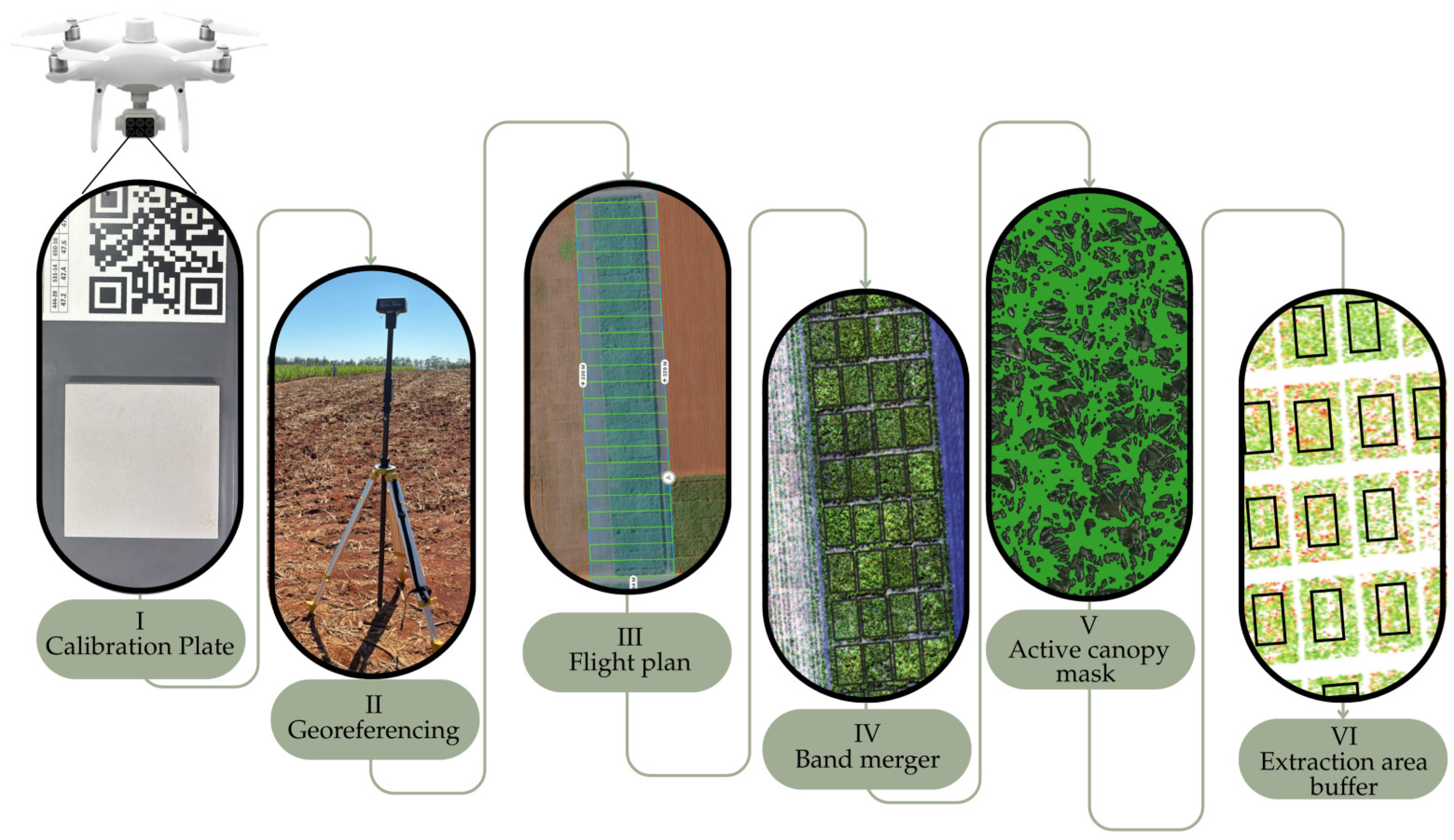
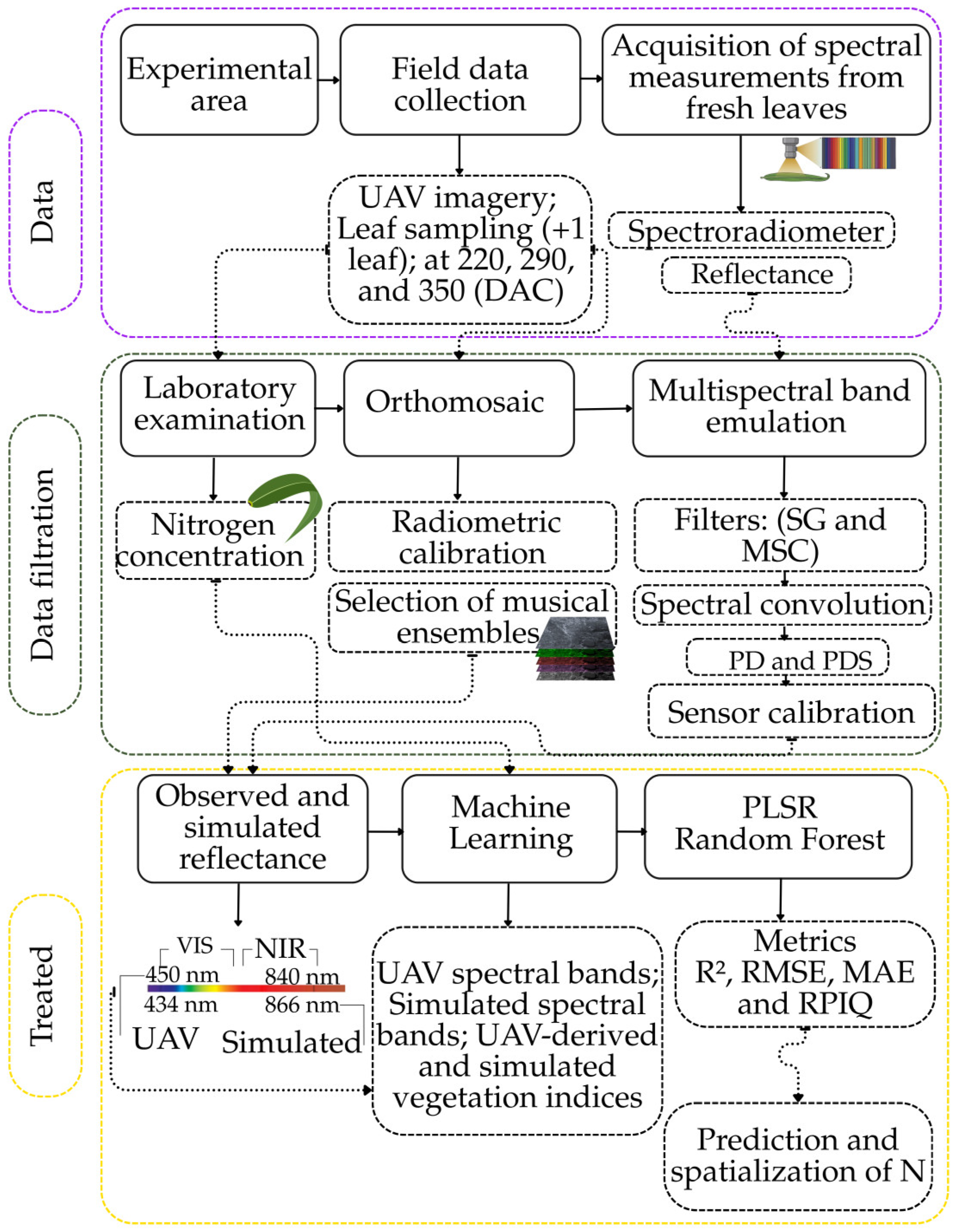
The methodology adopted in this study was structured into eight main stages: (i) setting up and conducting the field experiment; (ii) acquisition of multispectral data using UAVs; (iii) acquisition of hyperspectral and laboratory data (Leaf +1); (iv) preprocessing and extraction of spectral signatures in QGIS; (v) standardization and preprocessing of hyperspectral data; (vi) simulation of multispectral bands from hyperspectral leaf data; (vii) calculation of spectral indices (Sis) and predictive modeling of TFN; and (viii) prediction and spatialization of nitrogen (N) in the experimental area.

This methodological workflow enabled the integration of reflectance data obtained by a multispectral sensor mounted on a UAV, benchtop hyperspectral data, and laboratory analyses, allowing for the evaluation of the potential of spectral simulation regarding cross-domain calibration and the generalization of predictive N models in sugarcane. The study steps are presented in Figure 1.

Figure 1. Methodological workflow.

Figure 1. Methodological workflow.

2.1. Study Area and Experimental Conditions

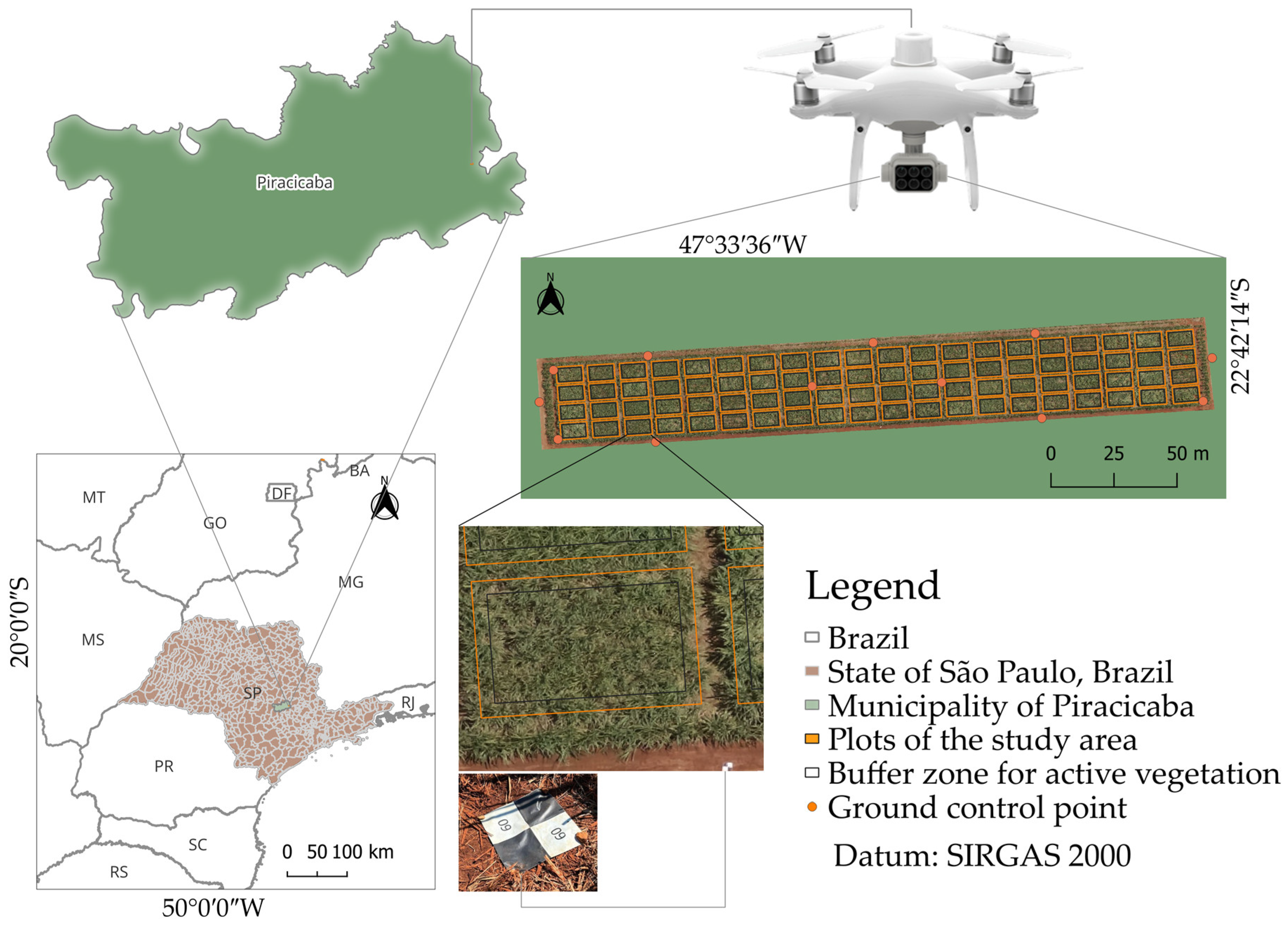
The experiment was conducted at a research site located at the Sugarcane Technology Center (CTC) in the municipality of Piracicaba, state of São Paulo, at geographic coordinates 22°42′15″ south latitude and 47°33′34″ west longitude, as shown in Figure 2. The soil in the experimental area is classified as Red-Yellow Argisol (PVA), the region’s climate is humid subtropical (CWa), according to the Köppen–Geiger classification, featuring hot and rainy summers and dry winters, with an average annual precipitation of less than 1400 mm [17].

2.2. Field Experimental Design

The experiment was conducted using a randomized block factorial design with four blocks, five sugarcane varieties (CT01, CT02, CT03, CT04, and CT05), and four nitrogen treatments, totaling 80 experimental plots in the third year of crop growth. Four sources of N variation were used: control (T1—no application), conventional (T2—1.0 kg t⁻¹), optimized 1 (T3—1.2 kg t⁻¹), and optimized 2 (T4—1.2 kg t⁻¹). Within each block, treatments were distributed by randomization, ensuring complete randomization. The replicates corresponded to the four blocks, so that each combination of variety and treatment was represented once in each block. Each experimental plot consisted of six rows, 15 m long and 9 m wide. It should be noted that the smaller area used in the spectral extraction stages corresponded only to the usable area of the plot, defined to reduce edge effects, without altering the replication structure of the experimental design.

2.3. Acquisition of Multispectral Images Using a UAV

The images were acquired using a multispectral sensor mounted on the DJI Phantom 4 Multispectral, P4M RTK unmanned aerial vehicle (UAV) (DJI Technology, Shenzhen, China). The system consists of five multispectral cameras covering the Blue (B), Green (G), Red (R), RedEdge (RE), NIR, and RGB bands (

Table 1. Characteristics of the multispectral sensor mounted on the UAV, including central wavelength (nm) and bandwidth (nm).

Band (λ)	Central Wavelength (nm)	Bandwidth (nm)
Blue (B)	450	±16
Green (G)	560	±16
Red (R)	650	±16
RedEdge (RE)	730	±16
NIR (NIR)	840	±26
RGB	20 megapixels

). Additionally, the equipment features an RTK (Real-Time Kinematic) module, which ensures greater accuracy in the georeferencing of the collected data.

Three flights were conducted 220, 290, and 350 days after cutting (DACs), between 10:00 a.m. and 11:00 a.m., following the same flight plan for all campaigns. The images were acquired at an altitude of 50 m, resulting in a ground sample distance (GSD) of 3.0 cm, with 80% forward overlap and 70% side overlap. Geometric consistency between multi-temporal flights was ensured by standardizing these acquisition parameters, using the drone’s onboard RTK system in conjunction with a Trimble R4 RTK GNSS base station (Trimble Inc., Sunnyvale, CA, USA), and processing the products in the same coordinate system. Additionally, 12 Ground Control Points (GCPs) with known coordinates, distributed throughout the experimental area, were used to assess the geometric accuracy of the orthomosaics. The geometric accuracy metrics were obtained from the photogrammetric processing report generated in Agisoft Metashape, which indicated an RMSE of 2.06 cm in X, 1.03 cm in Y, 0.18 cm in Z, 2.30 cm in the XY plane, and 2.31 cm total error, in addition to a reprojection error of 1.11 pixels.

2.4. Acquisition of Leaf Samples

Leaf sampling was conducted by collecting six fresh sugarcane leaves and selecting the +1 leaf, which corresponds to the first fully expanded leaf [15]. Leaves were chosen at random within each plot, excluding those at the edges. After collection, the leaves were placed in plastic bags and transported in coolers with ice to the laboratory, where hyperspectral measurements were performed. This technique was adopted to preserve the turgidity and spectral properties of the leaves [18,19]. The measurements were taken on the middle third of each leaf. After obtaining the spectra, the leaves were sent for laboratory leaf analysis to determine TFN. The collections were made during the 2024/2025 growing season, when the crop was in its third year of cultivation (replanted stand). Leaf samples were collected on the same day as the drone flights, corresponding to 220, 290, and 350 days after cutting (DACs), in order to standardize multispectral and hyperspectral sampling.

2.5. Acquisition of Laboratory Hyperspectral Data

The hyperspectral spectra were obtained using the FieldSpec^® 3 benchtop spectroradiometer (Analytical Spectral Devices Inc., Boulder, CO, USA). The equipment operates in the 350–2500 nm range, segmented between the VIS and NIR regions with a 1.4 nm sampling interval and the short-wave infrared (SWIR) region with a 2 nm interval.

Measurements were conducted in a controlled environment using the Leaf Clip^® accessory [20], which ensures orthogonal geometry and constant light intensity, minimizing variations caused by sample positioning or the angle of incidence. To ensure data consistency, radiometric calibration was performed every 15 min, using the Lambertian surface integrated into the Leaf Clip^® as a reference standard, following ASD protocols and the methodology adopted by Fiorio et al. [15].

2.6. Spectral Data Preprocessing

2.6.1. Calibration and Extraction of UAV Multispectral Data

A total of 3870 aerial photographs were acquired over the course of three data collection campaigns. The images were downloaded and processed using Agisoft Metashape Professional Edition 2.0.1 [21], based on the Structure from Motion (SfM) technique. The photogrammetric processing involved the three-dimensional reconstruction of the scene, generating the orthomosaic of the study area. Additionally, to ensure the spectral consistency of the images, radiometric correction was performed by inserting photographs of the calibration plate obtained before and after each flight. This procedure enabled the standardization of reflectance values and resulted in the generation of an orthomosaic for each of the five corrected spectral bands from the multispectral sensor mounted on the UAV.

With the aim of extracting exclusively the spectral signature of the sugarcane canopy and reducing noise associated with the presence of exposed soil, image borders, and shading, in accordance with the procedures established by Picado et al. [22], the bands were imported into Quantum GIS [23], version 3.40. Initially, the Normalized Difference Vegetation Index (NDVI) was calculated to highlight vegetation response and minimize interference from pixels not representative of the canopy. For this calculation, a threshold of 0.65 was adopted, with pixels having higher values considered active vegetation. This procedure reduced the influence of extreme spectral values, particularly those associated with exposed soil, shading, and spectral responses below the established threshold, thereby excluding information that did not represent the crop’s active canopy. This cutoff value, as reported by Wang et al. [24], proved effective in highlighting the active canopy and increasing the accuracy of the spectral response. Based on this criterion, the QGIS Raster “Calculator” tool was used to generate a segmentation mask, delimiting exclusively the areas of active sugarcane canopy. Next, a buffer zone 10 m long by 6 m wide was applied to delineate only the usable area of the plot, eliminating the margins. Finally, zonal statistics were calculated, and the median reflectance values corresponding to each spectral band were obtained through tabulation. The use of the median per plot helped mitigate the influence of residual extreme values on the spectral representation of each experimental unit, as shown in Figure 3.

2.6.2. Standardization of Hyperspectral Data

The spectra were initially recorded in radiance levels (raw values) and converted to reflectance using ViewSpec Pro software (version 5.7). To represent each plot, the median of the leaf readings was used. In the next step, the reflectance spectra underwent a quality control and standardization process prior to band simulation. In this process, responses with evident noise or values outside the interquartile range of each plot were eliminated. Additionally, spectral cropping was performed to exclude unstable regions, such as the range below 400 nm, characterized by a low signal-to-noise ratio, and the sections adjacent to the detector junctions (~1000 and ~2500 nm), which do not correspond to the wavelengths parameterized by the Phantom 4 Multispectral sensor.

2.7. Methodological Sequence of the Simulation and Modeling Technique

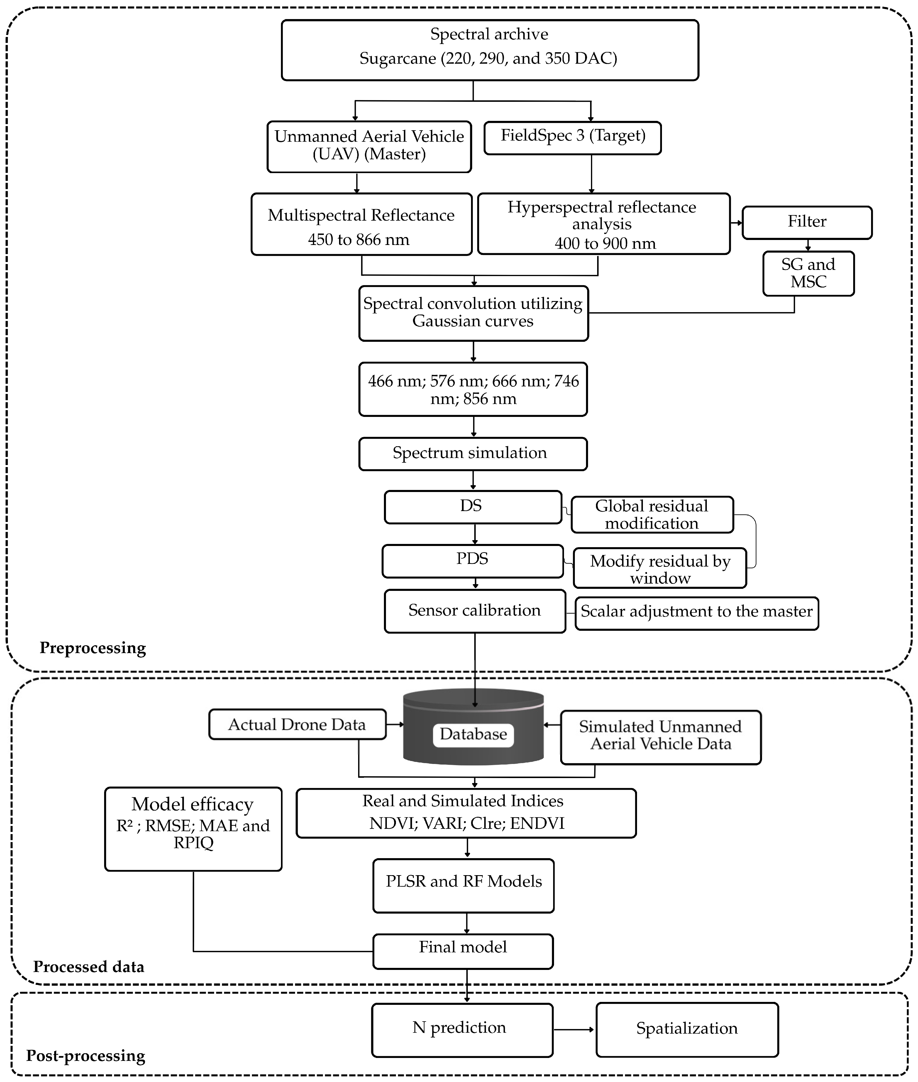
The flowchart illustrates the methodological steps followed to develop the spectral response simulation, in which canopy data obtained by UAV are used as a reference (master) for a hyperspectral leaf sensor (target), in order to make their spectral responses similar, as shown in Figure 4.

2.7.1. Spectral Convolution

For each plot, reflectance was represented by the median of the readings, generating a representative hyperspectral signature for each plot. Next, the spectra were cropped to the 400–900 nm range, with a continuous spectral resolution of 1.4 nm, in order to reduce interference outside the region of interest, standardize the analyzed spectral domain, and enable more consistent simulations across sensors. Subsequently, spectral preprocessing procedures were applied to minimize instrumental noise and light interference, using Multiplicative Signal Correction (MSC) and the Savitzky–Golay (SG) filter [25], implemented in RStudio [26] (version 4.5.0). MSC was employed to correct additive and multiplicative variations associated with light scattering among the samples, while the SG filter was used to smooth the spectral signatures, preserving the overall behavior of the reflectance curve. The MSC formulas are presented in Equations (1)–(3).

$${\mathrm{Spectra}}_{\mathrm{avg}}={\displaystyle \frac{{\displaystyle {\sum }_1^{\mathrm{n}}}{\mathrm{Spectra}}_{\mathrm{i}}}{\mathrm{n}}}$$

(1)

$${\mathrm{Spectra}}_{\mathrm{i}}=\mathrm{Ki} \times {\mathrm{Spectra}}_{\mathrm{avg}}+\mathrm{bi}$$

(2)

$${\mathrm{Spectra}}_{\mathrm{MSC},\mathrm{i}}={\displaystyle \frac{{\mathrm{Spectra}}_{\mathrm{i}} \mathrm{ }-\mathrm{ }\mathrm{bi}}{\mathrm{ki}}}$$

(3)

where

• Spectra_avg corresponds to the average of all leaf spectra;
• n represents the total number of spectral data points;
• Spectra_i refers to each individual leaf spectrum;
• ki and bi are correction coefficients obtained by linear regression from Spectraavg;
• Spectra_MSC,i corresponds to the spectrum corrected using the MSC method.

Next, spectral convolution was applied to reproduce the response of a multispectral sensor from the hyperspectral data, a procedure widely used in cross-validation and time-series integration [27]. For the DJI Phantom 4 Multispectral (P4M), the simulated reflectance of each band was calculated as a weighted average of the FieldSpec^® 3 reflectance using spectral response functions (Equation (4)), approximated by Gaussian curves, parameterized by the central wavelengths and full width at half maximum (FWHM) values provided by the manufacturer (Blue 450 ± 16 nm; Green 560 ± 16 nm; Red 650 ± 16 nm; RedEdge 730 ± 16 nm; NIR 840 ± 26 nm).

It should be noted that the P4M’s full spectral response functions (SRFs) are not provided by the manufacturer as detailed normalized curves; only the center wavelengths and bandwidths of each channel are officially reported. For this reason, the spectral simulation was conducted using a Gaussian approximation based on these parameters, which constitutes a methodological limitation of the study. It is recognized that the exact shape of the SRF can influence the simulated reflectance and, consequently, the modeling results. In the present work, however, the sensitivity of the results to the assumption of a Gaussian distribution of the SRFs was not evaluated in isolation. To mitigate potential biases arising from this simplification and align the spectral domains, the simulation was not used in isolation but followed by an inter-sensor calibration workflow involving Direct Standardization (DS), Piecewise Direct Standardization (PDS), affine band-wise adjustment, and quantile-based constraint to the master sensor, as described in the subsequent sections.

$${\mathrm{R}}_{\mathrm{b}}{\displaystyle \frac{{\mathsf{\Sigma }}_{\mathrm{i}=1}^{\mathrm{n}} \mathrm{R}\left(\mathsf{\lambda }\mathrm{i}\right)\mathrm{SRFb}\left(\mathsf{\lambda }\mathrm{i}\right)\mathsf{\Delta }\mathsf{\lambda }\mathrm{i}}{{\mathsf{\Sigma }}_{\mathrm{i}=1}^{\mathrm{n}} \mathrm{SRFb}\left(\mathsf{\lambda }\mathrm{i}\right)\mathsf{\Delta }\mathsf{\lambda }\mathrm{i}}}$$

(4)

where

• Rb is the simulated reflectance of the band;
• b, λi are the wavelengths measured by the FieldSpec;
• Δλi is the spectral resolution (1.4 nm), and the denominator ensures normalization, and
• SRFb (λi) corresponds to the spectral response function of band b.

2.7.2. Transfer Calibration Using (DS/PDS)

Cross-calibration between spectral domains was performed using Direct Standardization (DS) and Window Direct Standardization (PDS), classical calibration transfer techniques [28,29]. The DS method is based on establishing a global spectral transfer matrix derived from the mathematical relationship between the spectra of a set of standard samples measured by the master instrument and the spectra measured by the target instrument.

On the other hand, PDS is better at capturing variations dependent on the local wavelength, i.e., by windows. From these coefficients, a transfer matrix is constructed and applied to the spectra of the target instrument in order to maximize similarity with the spectra of the reference (master) instrument.

In the context of PDS, the window width (ω) is a key hyperparameter, as it balances the trade-off between local accuracy, typically associated with narrow windows, and numerical robustness, generally favored by wider windows; it is therefore defined empirically [30]. In this work, the methodological strategy consisted of integrating DS and PDS, adopting a window width corresponding to five wavelengths, aligned with the number of evaluated bands.

This choice allowed for consistent local corrections, reduced the dimensionality within each window, and contributed to greater numerical stability. Thus, the spectral segmentation adopted in PDS preserved the flexibility inherent to DS while minimizing the number of hyperparameters to be adjusted [31].

In this study, the multispectral sensor mounted on the UAV was defined as the master, since it serves as the spectral reference and the target calibration scale. The actual bands captured by the UAV represent the comparison standard, such that all transformations aim to align the simulated spectra with this domain. Thus, the quality of the standardization process was evaluated based on the correspondence between the corrected data and the original measurements of the master.

The hyperspectral spectrum obtained in the laboratory, after convolution with the estimated spectral response functions (SRFs), was defined as the target, as it represents the source to be adjusted to the master. The sequential application of DS, PDS, and scalar adjustment aims to transform the simulated spectra, reducing instrumental discrepancies and maximizing similarity with the actual bands of the UAV. Thus, the (hyperspectral) target corresponds to the corrected spectral domain, whose performance is continuously evaluated relative to the master (UAV).

2.7.3. Sensor-to-Sensor Calibration

After simulating the multispectral bands from the hyperspectral spectra, a sequential inter-sensor calibration procedure was performed separately for each DAC, with the aim of aligning the simulated values with the radiometric scale of the RPA’s multispectral sensor. This type of harmonization is particularly relevant when there are instrumental differences between sensors and between their spectral response functions, which can directly affect the comparability between bands and indices derived from different platforms [6,32]. Initially, Direct Standardization (DS) with ridge regularization was applied to promote a global alignment between the simulated signals and the drone’s actual measurements. Next, the remaining residuals were modeled using Piecewise Direct Standardization (PDS) in local windows per band, allowing for refinement of the spectral fit. The adoption of this approach is consistent with the fundamentals of inter-instrument calibration transfer, widely employed to reduce systematic discrepancies between measurement platforms [33].

Subsequently, a band-specific adjustment was applied using linear regression between the corrected values and the values observed on the master sensor, with the aim of correcting any remaining offset and scale errors after the DS and PDS steps. Next, the calibrated signals were clipped to the 1st and 99th quantiles of the drone’s reflectance distributions to avoid extrapolation and preserve the physical consistency of the final values. In addition, the possible effects of mixed pixels and edges were minimized through the spatial processing described in Section 2.6.1, including canopy segmentation, the exclusion of pixels not representative of active vegetation, the application of a buffer to delimit the usable area of the plots, and the use of the spectral median per plot. These procedures were adopted to reduce the influence of bare soil, shading, and edges on the values used in calibration and modeling. The performance of the cross-sensor calibration step was evaluated by band based on the RMSE, as shown in

Table 2. Comparison of error by band before and after the final calibration adjustment between sensors, on different acquisition dates (DACs).

DAC	Band	RMSE (DS + PDS)	RMSE (Affine + Clamp)	Reduction (%)
220	Blue	0.0018265	0.0018113	0.83
220	Green	0.0034997	0.0034837	0.46
220	Red	0.0024439	0.0024354	0.35
220	RedEdge	0.0091257	0.0090916	0.37
220	NIR	0.0171810	0.0171629	0.10
290	Blue	0.0011469	0.0011469	0.00
290	Green	0.0025482	0.0025478	0.01
290	Red	0.0023208	0.0023189	0.08
290	RedEdge	0.0043149	0.0043131	0.41
290	NIR	0.0057761	0.0057583	0.31
350	Blue	0.0020088	0.0020067	0.10
350	Green	0.0039361	0.0039333	0.07
350	Red	0.0046349	0.0046324	0.05
350	RedEdge	0.0046667	0.0046307	0.70
350	NIR	0.0078339	0.0078085	0.33

RMSE (DS + PDS) corresponds to the error obtained after the Direct Standardization and Piecewise Direct Standardization steps. RMSE (affine + clamp) corresponds to the error after affine adjustment by band and the constraint to the quantiles of the master sensor. RMSE (DS + PDS) corresponde ao erro obtido após as etapas de Direct Standardization e Piecewise Direct Standardization. RMSE (afim + clamp) corresponde ao erro após o ajuste afim por banda e a restrição aos quantis do sensor mestre. The reduction (%) expresses the significant relative gain achieved by the final discovery step compared to the error obtained after DS + PDS.

.

2.7.4. Nitrogen-Sensitive Vegetation Indices

The spectral bands extracted from the sugarcane orthomosaic were used to calculate spectral indices (SIs), defined as transformations obtained by combining two or more multispectral bands. In this study, the selection of these indices was guided by their higher correlation with foliar nitrogen content TFN, as they can capture variations related to pigmentation, photosynthetic activity, and canopy structure [6,34].

To ensure comparability between the datasets, the SIs were calculated based on the spectral bands extracted from the buffer of each experimental plot. For the simulated data, the same spatial and spectral representation was adopted; that is, the values were organized to correspond to the same plots and the same set of bands considered in the observed data. This ensured standardization of the unit, allowing for consistent comparisons. Furthermore, the same indices were calculated for both domains (

Table 3. List of vegetation indices used in the modeling, along with their respective equations and references. The Blue, Green, Red, RedEdge, and NIR bands are represented by B, G, R, RE, and NIR, respectively.

ID	Vegetation Index	Formula	References
1	Normalized Difference Vegetation Index (NDVI)	(NIR − R)/(NIR + R)	[35]
2	Visible Atmospheric Resistance Index (VARI)	(G − R)/(G + R − B)	[36]
3	Chlorophyll Index—RedEdge (ChlRe)	(NIR)/(RED) − 1	[37]
4	Improved Normalized Difference Vegetation Index (ENDVI)	((NIR − G) − (2 × B))/((NIR − G) + (2 × B))	[38]

), which ensured methodological uniformity and greater robustness in the evaluation of TFN. Given the objective of comparing compatible spectral domains, the modeling was restricted to spectral bands and spectral indices common to both the data observed by RPA and the data simulated from the foliar hyperspectral domain.

2.8. Spearman Correlation

To investigate the relationship between the bands obtained by UAV, the simulated bands, and the SIs derived from both sources, we used Spearman’s correlation coefficient, a widely used nonparametric technique for measuring the strength and direction of monotonic associations between variables. This coefficient is particularly suitable when the data do not meet the assumptions of normality or when the relationship between variables is not strictly linear, and it is calculated based on the ranking of the observed values. Its values range from −1 to 1, where positive coefficients indicate direct monotonic associations, negative coefficients indicate inverse associations, and absolute values closer to 1 represent stronger relationships between the analyzed variables [39,40].

2.9. Modeling of Nitrogen Content Using Machine Learning

2.9.1. Linear Regression

Linear regression is one of the simplest and most widely used statistical techniques, designed to model the relationship between a dependent variable (SIs) and an independent variable (TFN). This technique assumes that there is a linear relationship between the variables and is commonly tested using the p-value associated with the model’s slope coefficient, where values of p < 0.001 indicate that this relationship is statistically significant [41]. Linear regression provides a simple and effective basis for estimating foliar nutrients based on spectral data, allowing for the quantification of the strength and direction of the association between SIs and TFN.

2.9.2. Partial Least Squares Regression (PLSR)

The Partial Least Squares Regression (PLSR) machine learning technique was used with the NIPALS algorithm. This technique was used to estimate nutritional content based on the reflectance of multispectral (canopy) and simulated (foliar) data. PLSR is widely used in predictive analyses with spectral data, as it projects the original variables into a reduced-dimensional space composed of latent variables (or factors). During the calibration process, the model simultaneously integrated information from correlated independent variables (spectral bands and indices) and dependent variables (TFN), seeking to identify the minimum number of factors necessary to explain the variability in the responses. Furthermore, PLSR stands out for its ability to mitigate multicollinearity among independent variables. This characteristic is especially relevant in hyperspectral data, where the strong correlation between adjacent bands compromises the application of conventional methods. In addition to overcoming this challenge, PLSR extracts latent components that condense the variability of the spectra and simultaneously explain multiple variables of interest, resulting in robust and stable models, as has already been demonstrated in various studies [4,42].

Excessive use of latent components may lead the model to interpret noise as relevant signal, resulting in inferior predictive performance, with increasing overfitting effects as more factors are included than necessary [13,43]. Thus, a well-balanced model should combine quality and predictive power, making it suitable for use in remote sensing studies focused on plant nutrition. For PLSR, the parameterization was partially optimized, since the number of latent components (ncomp) was not set manually but selected based on the performance obtained in a 10-fold cross-validation, with an automatic search defined by tuneLength = 15. In contrast, the preprocessing of the predictor variables (spectral bands and SIs) was kept fixed, with centering and scaling. After defining the final model, the variable importance in projection (VIP) analysis was performed, calculated based on the loading weights, scores, and the contribution of the selected components to the explained variance of the response variable, allowing the identification of the most relevant predictors for estimating the TFN.

2.9.3. Random Forest (RF)

The Random Forest (RF) model was applied; it is widely used in high-dimensional data processing and is one of the most commonly adopted methodologies for handling hyperspectral data [6]. RF is an algorithm developed by Breiman [44], frequently used independently for regression and classification problems. This method employs a bootstrap aggregation or bagging process, in which each tree is trained on a subsample of the initial dataset. Thus, each tree contributes an individual prediction. The combination of these predictions resulted in the final estimate [45]. During the prediction process, the model used the average or majority of the predictions, ensuring a balance in the error of each tree. This improved the model’s generalization ability [46].

The RF model relies on the prior definition of hyperparameters. In this study, the following values were empirically selected, ntree = 1000, mtry = 9, min.node.size = 20, and splitrule = “variance,” which were kept fixed during training. Thus, the model was not subjected to a formal systematic optimization of the hyperparameters, and its robustness was evaluated by 10-fold cross-validation. The choice of these values was based on empirical criteria and recommendations from the literature, such as those presented by Chen et al. [43], with the aim of reducing the occurrence of inappropriate configurations and improving the stability of the fit. Although this strategy does not exhaustively explore the hyperparameter space, the parameters used were explicitly reported, preserving the reproducibility of the adopted procedure.

In addition, we chose to use PLSR and RF because they represent well-established and widely used approaches in spectral modeling, accounting for both linear and nonlinear relationships. Although more complex methods, such as deep learning, may offer high predictive potential, their application was not prioritized in this study due to the comparative nature of the research and the structure of the available dataset. In general, deep learning approaches require a larger sample size, as well as additional regularization and validation strategies, in order to reduce the risk of overfitting and increase the robustness of generalization. Thus, the choice of PLSR and RF was aligned with the study’s methodological proposal and the search for comparable, robust, and interpretable models.

2.9.4. Performance Indicators

The quality of the models for predicting TFN in sugarcane was assessed by comparing the observed values with those predicted by the models. For these analyses, validation metrics such as the coefficient of determination (R²), root mean square error (RMSE), mean absolute error (MAE), and the ratio of performance to interquartile range (RPIQ) were used, whose mathematical expressions are presented in Equations (5)–(8). According to Rodrigues et al. [47], R² classifies prediction models as follows: poor (≤0.50), moderate (0.50–0.65), good (0.65–0.80), very good (0.80–0.90), and excellent (≥0.90).

$$\mathrm{R}2=\mathrm{ }{\displaystyle \frac{[\mathsf{\Sigma }\left(\mathsf{\gamma }\mathrm{p}\mathrm{ }-\mathrm{ }\underset{\_}{\mathsf{\gamma }}\mathrm{p}\right) .\mathrm{ }\mathrm{ }\left(\mathsf{\gamma }\mathrm{o}\mathrm{ }-\mathrm{ }\underset{\_}{\mathsf{\gamma }}\mathrm{o}\right){]}^2}{[\mathsf{\Sigma }{\left(\mathsf{\gamma }\mathrm{p}\mathrm{ }-\mathrm{ }\underset{\_}{\mathsf{\gamma }}\mathrm{p}\right)}^2.{\left(\mathsf{\gamma }\mathrm{o}\mathrm{ }-\mathrm{ }\underset{\_}{\mathsf{\gamma }}\mathrm{o}\right)}^2]}}$$

(5)

$$\mathrm{RMSE}= \sqrt{{\displaystyle \frac{{\sum }_{\mathrm{i}=1}^{\mathrm{n}}({\widehat{{\mathrm{y}}_{\mathrm{i}}}-{\mathrm{y}}_{\mathrm{i}})}^2}{\mathrm{n}}}}$$

(6)

$$\mathrm{MAE}= {\displaystyle \frac{1}{\mathrm{n}}} \sum _{\mathrm{i}=1}^{\mathrm{n}}\left|{\mathrm{X}}_{\mathrm{i}}- \mathrm{X}\right|$$

(7)

$$\mathrm{RPIQ}={\displaystyle \frac{{\mathrm{IQR}}_{\mathrm{obs}}}{\mathrm{RMSE}}}$$

(8)

To ensure the robustness and generalizability of the models, two complementary validation strategies were adopted. The first used k-fold cross-validation (k = 10), in which the set of 240 observations was divided into ten balanced subsets; in each iteration, nine subsets were used for training and one for validation, ensuring that all data were tested at least once. The second strategy applied the hold-out method, partitioning 70% of the data for training and 30% for independent testing. For cross-domain validation, this division was based on nitrogen levels to preserve the distribution of the response variable across the subsets. However, the partition was not simultaneously stratified by block and variety, and this aspect should be considered when interpreting the robustness of the independent validation. Repeated cross-validation was not employed. This combined approach allowed for the evaluation of model performance both during training and on an independent dataset, helping to mitigate the risk of overfitting and providing a more robust estimate of generalization ability.

3. Results

3.1. TFN and Precipitation Throughout the Season

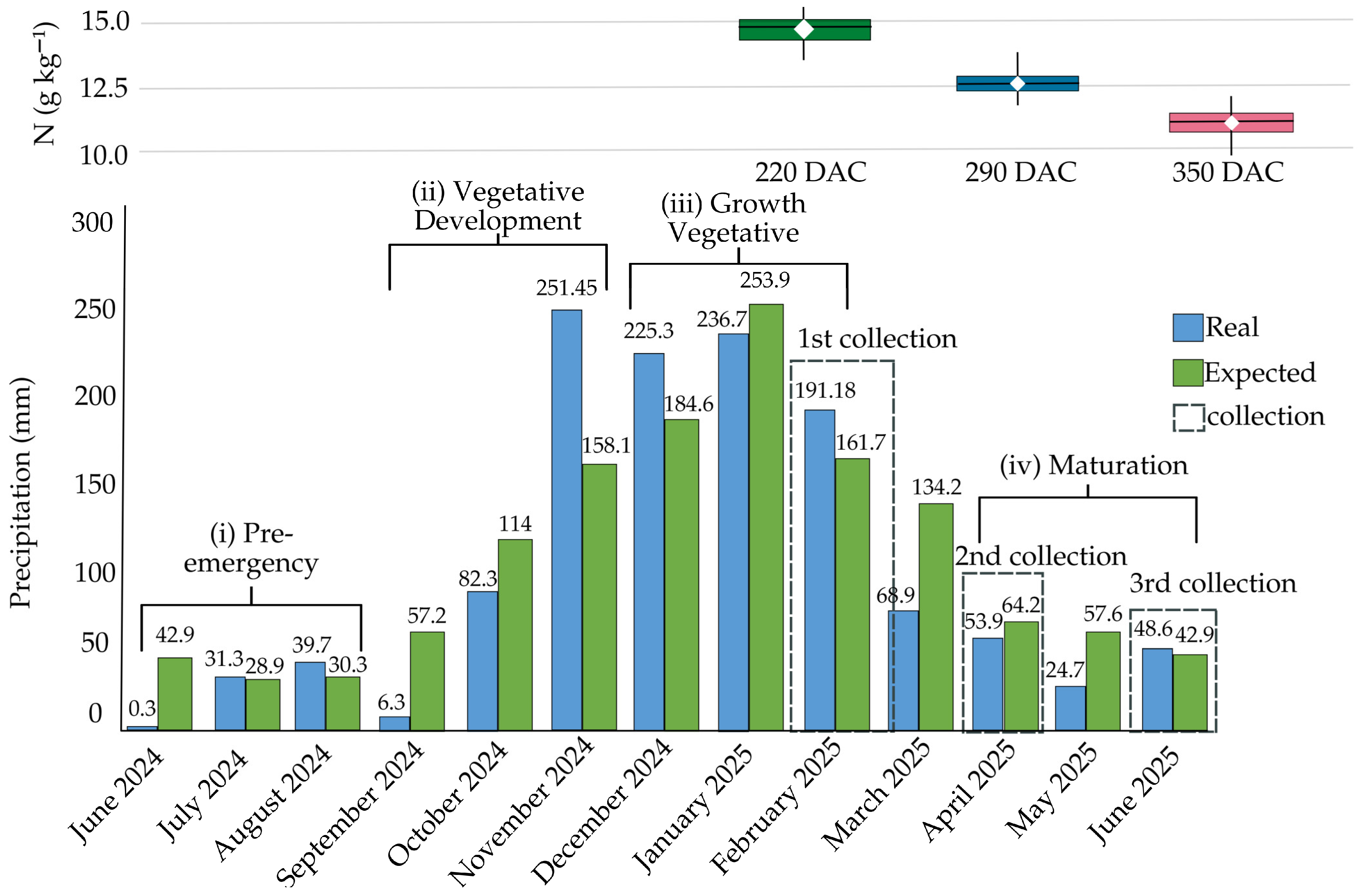
Figure 5 shows precipitation throughout the 2024/2025 sugarcane growing season, along with nitrogen data for the respective samples collected at 220, 290, and 350 days after planting. The phenological cycle of sugarcane consists of four stages: (i) pre-emergence from 0 to 90 days, (ii) vegetative development from 90 to 180 days, (iii) vegetative growth from 180 to 270 days, and (iv) maturation from 270 to 360 days. Among these stages, vegetative development is the one with the highest nutrient concentrations in the plantation [22]. A water deficit was observed during the initial months of the 2024 harvest season, from June to October, corresponding to a phase of extreme importance for the crop’s vegetative development.

Precipitation patterns throughout the sugarcane growing cycle were consistent with the crop’s physiological demands at each phenological stage. Although a slight water deficit was observed at the beginning of the growing season, the crop showed satisfactory development in later stages. This behavior is consistent with the variation in TFNs throughout the harvesting periods, since, during vegetative growth, greater water availability promotes photosynthetic activity, canopy expansion, and N uptake [15].

In contrast, the reduction in TFN levels at 290 and 350 DAC, at the onset of maturation, may reflect both the physiological changes inherent to the progression of the growth cycle and the internal redistribution of the nutrient, with a decrease in its concentration in the leaves and a greater allocation of assimilates to the stems [48].

3.2. Spearman’s Correlation Between Original and Simulated Bands and Indices in Relation to the TFN

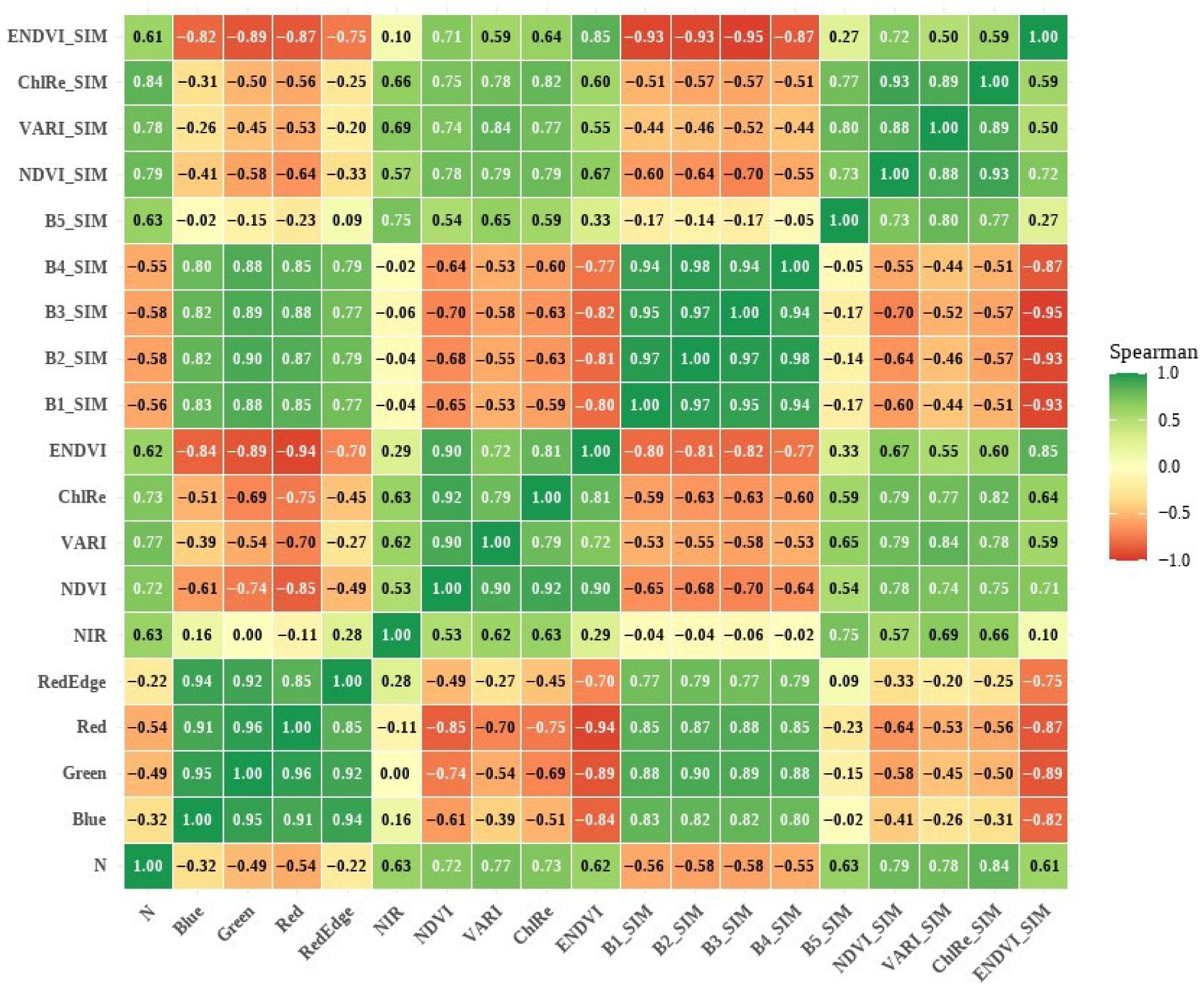
In this study, Spearman’s correlation coefficient (r) was used to assess the association between TFN and the reflectance values of the original and simulated bands, as well as the spectral indices (SIs) calculated from these bands. The analysis focused on the Blue, Green, Red, RedEdge, and NIR spectral regions due to their greater interaction with chlorophyll and pigments directly involved in the photosynthetic process and, consequently, closely related to TFN. Thus, the DAC dataset was considered, which enabled a more robust assessment of the relationship between the variables under different conditions, as illustrated in Figure 6.

The spectral bands and SIs showed consistent associations with TFN, with negative correlations in the VIS spectrum and positive correlations in the NIR. The spectral bands and (SI) showed associations in different directions, with negative correlations in the VIS spectrum and positive correlations in the NIR. In the bands obtained by UAV, for example, the “r” values were −0.32, −0.49, −0.54, and −0.22 for Blue, Green, Red, and RedEdge, respectively, while in the NIR, r = 0.63.

The simulated bands reproduced a similar correlation pattern, but with more pronounced magnitudes (B1SIM r = −0.56; B2SIM r = −0.58; B3SIM r = −0.58; B4SIM r = −0.55; B5SIM r = 0.63), indicating consistency between the simulation and the original data. This result indicates a stronger association between chlorophyll content and higher photosynthetic activity, which increases absorption in the VIS region, particularly in the Blue, Green, and RedEdge regions. In contrast, the signal in the NIR is more influenced by multiple scattering linked to the internal structure of the leaf and canopy architecture, which may support the positive correlation observed in this spectral region.

The SIs showed a similar correlation with TFN in the assessed domains, where for NDVI, r = 0.72 and simulated r = 0.79; for VARI, r = 0.77 and simulated r = 0.78; for ChlRe, r = 0.73 and simulated r = 0.84; and for ENDVI (r = 0.62; simulated r = 0.61). Furthermore, the indices derived from the simulated bands generally showed slightly higher correlations than those obtained with the original data, which is consistent with the origin of the bands: since they are constructed from narrow-band spectral information, they tend to better preserve subtle spectral features and, consequently, respond to small variations related to chlorophyll and N.

Finally, the comparison between indices calculated from actual UAV data and those derived from simulated data revealed the following correlations: NDVI vs. simulated (r = 0.78), VARI vs. simulated (r = 0.84), ChlRe vs. simulated (r = 0.82), and ENDVI vs. simulated (r = 0.85). Taken together, these results indicate high agreement between the indices obtained from the bands measured by the UAV and those generated from the simulated bands, suggesting that the simulation adequately preserved the spectral behavior necessary to reproduce the patterns captured by the indices and, consequently, reinforcing the consistency and usefulness of both datasets.

3.3. Exploratory Estimation of TFN Sugarcane Using SIs from UAV Data and Derived from the Simulated Dataset

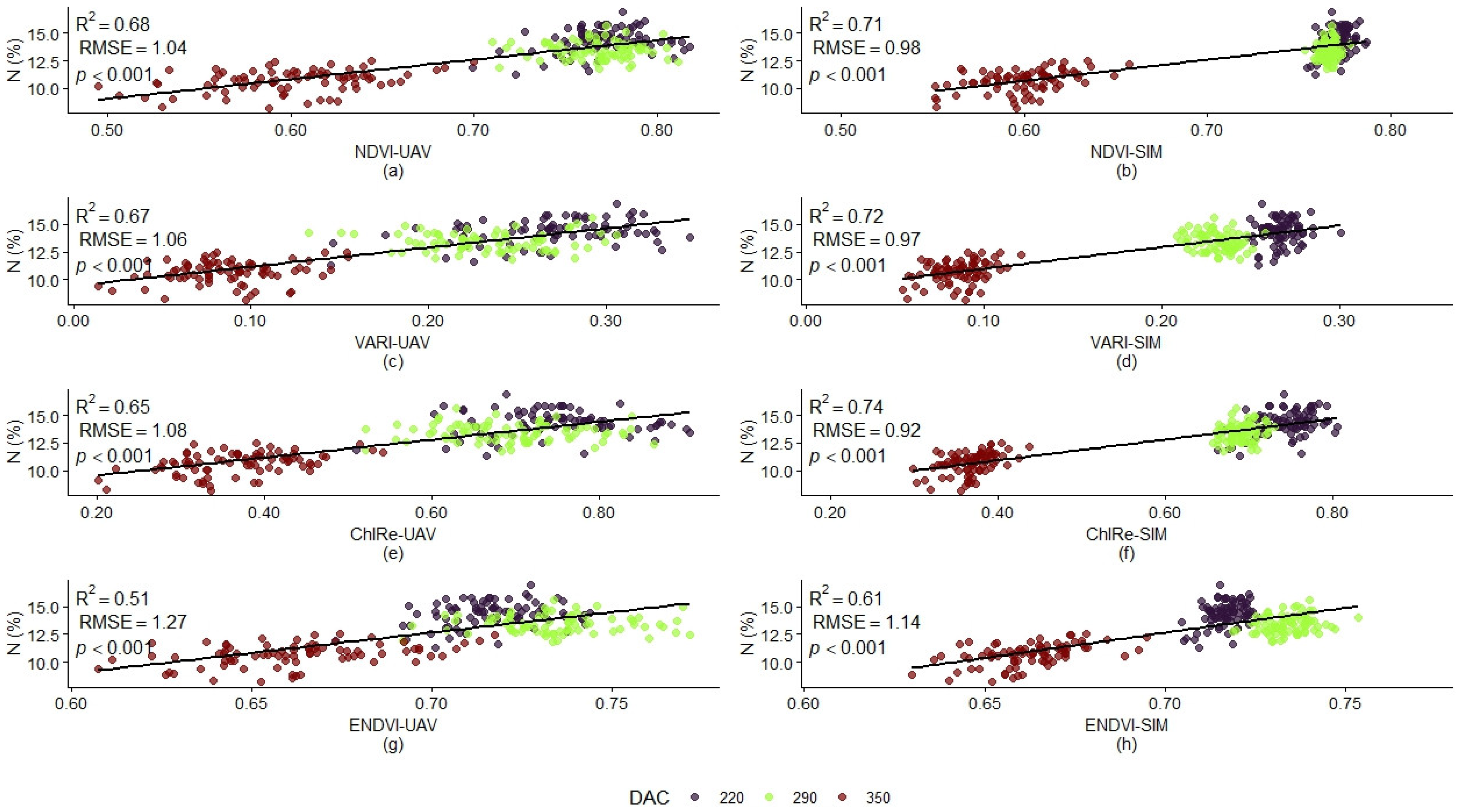
Figure 7 shows the linear regression between N concentration (%) and the spectral indices (SIs) used in this study (NDVI, VARI, ChlRe, and ENDVI), calculated from actual UAV data and their corresponding simulated (SIM) values in relation to their phenological stage in the DACs. These SIs summarize differences in reflectance in specific regions of the spectrum and, therefore, serve as compact descriptors of the biophysical and biochemical state of the vegetation.

The indices calculated from the canopy’s spectral response were statistically significant (p < 0.001) for TFN estimation, with performance ranging from “good” to “moderate.” The NDVI, for example, showed R² = 0.68 and RMSE = 1.04, followed by the other indices (VARI, R² = 0.67, RMSE = 1.06; ChlRe, R² = 0.65, RMSE = 1.08; ENDVI, R² = 0.51, RMSE = 1.27). The SIs obtained from the spectral response of the simulated data reproduced the trend observed in the SIs derived from UAV data, but with more clearly defined associations regarding TFN and the different DACs. This behavior can be explained by the nature of the simulated data, whose origin favors a more sensitive spectral response and one less subject to canopy interference, allowing for the capture of variations related to the leaf’s nutritional status with greater discrimination. In this dataset, NDVI (R² = 0.71 and RMSE = 0.98), VARI (R² = 0.72 and RMSE = 0.97), and ChlRe (R² = 0.74 and RMSE = 0.92) performed satisfactorily, while ENDVI showed lower performance (R² = 0.61; RMSE = 1.14).

3.4. Modeling of TFN Using a UAV-Derived Spectra and Simulated Data

The sugarcane TFN prediction model was developed using original multispectral data and simulated spectral data obtained during the stump development phase. For modeling, two widely established algorithms in spectral analysis were employed: PLSR [49] and RF [50].

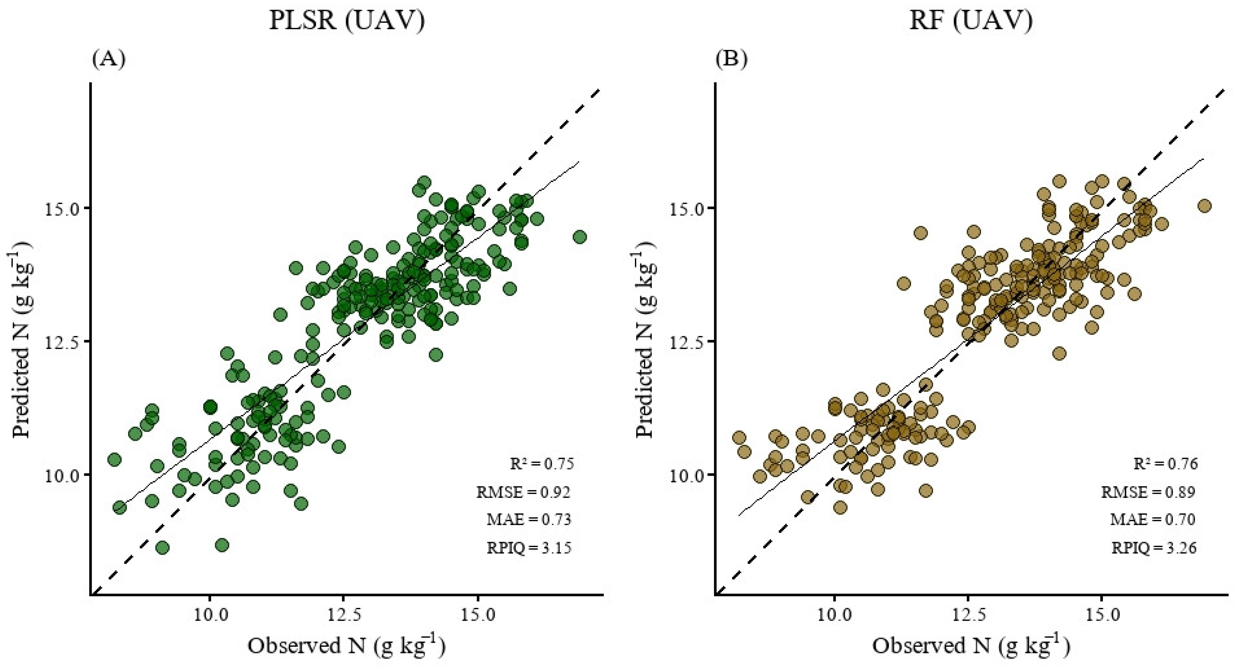
In this context, both models demonstrated good predictive capability for the UAV data (Figure 8B). The PLSR model showed “good” performance, with an R² of 0.75, an RMSE of 0.92 g kg⁻¹, an MAE of 0.73, and an RPIQ of 3.15. Similarly, the RF model also showed satisfactory performance, with an R² of 0.76, an RMSE of 0.89 g kg⁻¹, an MAE of 0.70, and an RPIQ of 3.26.

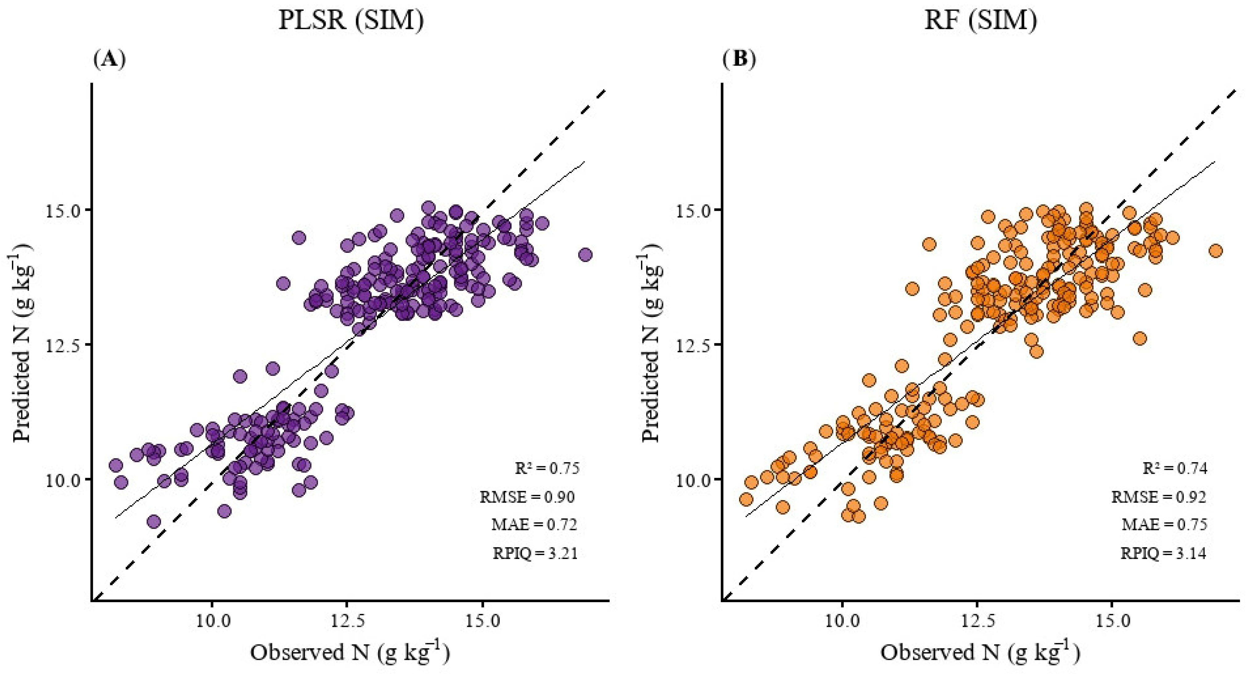
Similar results were also observed for the models calibrated using the simulated data, where PLSR yielded R² = 0.75, RMSE = 0.90 g kg⁻¹, MAE = 0.72, and RPIQ = 3.21, while RF generated R² = 0.74, RMSE = 0.92 g kg⁻¹, MAE = 0.75, and RPIQ = 3.14 (Figure 9A,B).

Overall, the performance of the models calibrated using data collected from the crop canopy via UAV and data simulated from leaf spectral curves showed similar values across all indicators and performed well, indicating that the methodology employed was able to satisfactorily reproduce the spectral behavior observed in the real data.

3.5. Variable Importance in Projection (VIP)

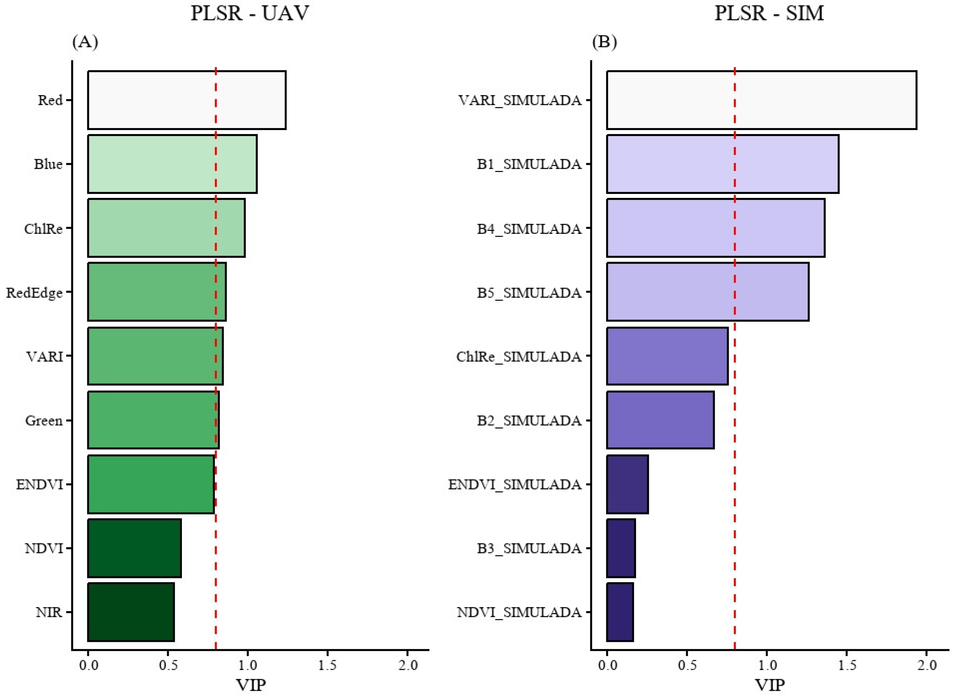
Analysis of the VIP values for the PLSR model (Figure 10A,B) revealed the variables that contributed most to the prediction of TFN. In the original canopy data, the Red, Blue, and RedEdge bands stood out in that order of importance, in addition to the ChlRe and VARI indices. For the simulated data, the most relevant variables include the Blue, RedEdge, and NIR bands, as well as the VARI, in that order. In both datasets, these variables exceeded the heuristic threshold of 0.8, indicating an above-average contribution to explaining TFN variability.

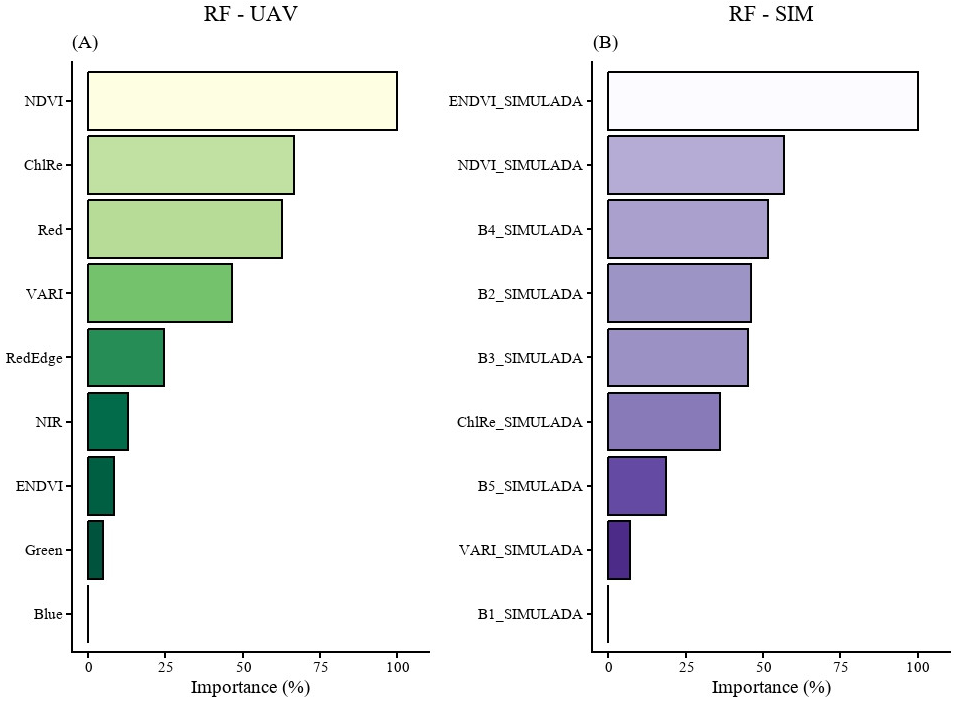
In contrast, the importance of variables by permutation was estimated by randomizing the values of each predictor, followed by an assessment of the impact of this change on the model’s overall performance, as shown in (Figure 11A,B). In the RF model, this approach revealed a more concentrated distribution of predictive relevance across a smaller number of variables. In the UAV dataset, the NDVI, Clre, and VARI indices stood out, in addition to the Red band. In the simulated dataset, however, the greatest contributions were observed for the ENDVI_SIM and NDVI_SIM indices, as well as for the RedEdge and Green bands (B4 and B3_SIM), as shown in Figure 9A,B. This behavior is consistent with the structural differences between the evaluated models.

3.6. Independent Validation

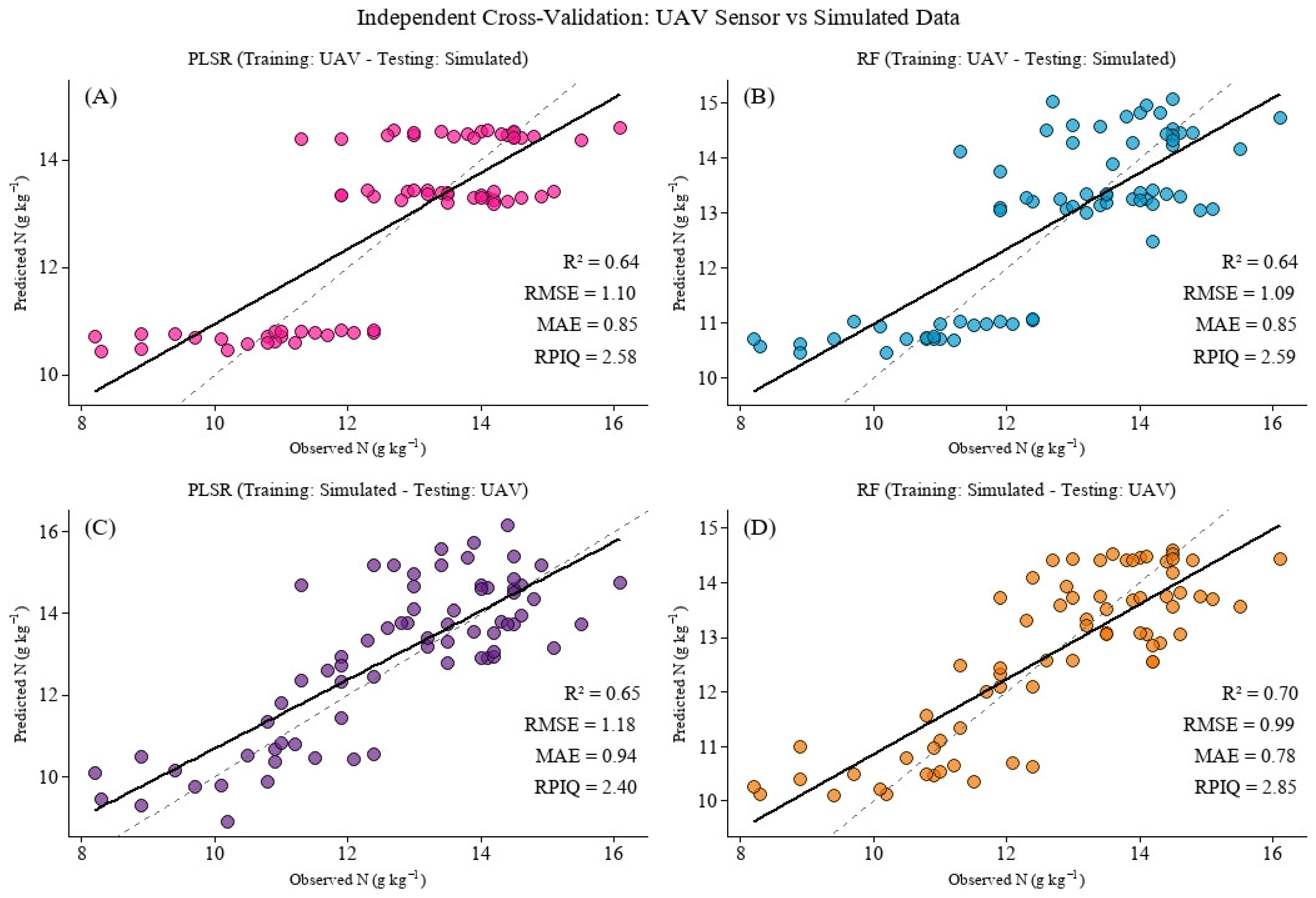
In this step, the hold-out validation technique was employed, in which 70% of the data were allocated to training and 30% to validation on an independent dataset. This division was based on nitrogen levels, in order to preserve the distribution of the response variable between the training and test sets. This procedure was used to analyze model transfer between the RPA (original) and simulated domains in TFN prediction (Figure 12), comparing the PLSR and RF algorithms. It should be noted, however, that this transfer was evaluated between distinct data domains, though generated under the same experimental context, involving the same location, growing season, and set of varieties.

Panels A and B show the models calibrated using the RPA’s spectral bands and SIs, which were subsequently applied to the simulated bands and spectral indices. Panels C and D, on the other hand, show the reverse procedure, in which the models were trained on the simulated data and evaluated on the RPA data, using the same validation criteria.

The transferability of TFN models between domains (UAV and SIM), comparing PLSR and Random Forest in both transfer directions, yielded “moderate” results in scenarios (A, B, and C), with R² > 0.64, demonstrating that there is a stable relationship between the domains, though with a loss of accuracy associated with the change in spectral representation. Notably, the RF trained on SIM data and tested on UAV data showed the best performance in terms of explanation and error (R² = 0.70; RMSE = 0.99 g kg⁻¹; MAE = 0.78; RPIQ = 2.85), demonstrating greater robustness of the nonlinear model.

3.7. Spatialization and Mapping of TFN

When comparing different modeling strategies for estimating TFN, it was found that the validated RF model exhibited the best predictive performance, even when applied to a reduced dataset. Due to its robustness and flexibility in handling high-dimensional spectral data and spatial variability, the RF model was selected for the spatialization stage. Previous studies show that RF provides more accurate predictions than traditional linear methods, in addition to allowing the integration of multiple spectral bands and environmental variables [51].

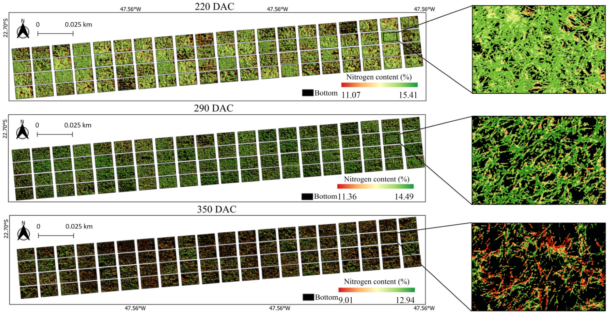
In addition to demonstrating statistical stability, the model proved capable of spatializing TFN, which strengthens its applicability in pixel-by-pixel prediction of multispectral images. Using the global model, applied to each scenario (220, 290, and 350 DAC), it was possible to generate a map of the spatial distribution of TFN in the experimental area, considering different phenological stages, as illustrated in Figure 13.

As shown in Figure 13, the estimated TFN in the leaf is represented by a color gradient, in which red tones indicate lower concentrations and green tones indicate higher concentrations, following the concentration scale. It is noted that N values gradually decrease throughout the growth phases, stem elongation, and the maturation phase; for example, at 220 DAC, the TFN ranges from 11.07 to 15.41 (%), while at 350 DAC, the TFN ranges from 9.01 to 12.94 (%). Furthermore, the spatial pattern obtained indicates good model performance, which maintained consistent predictions even when using simulated data, suggesting the ability to generalize across domains. This behavior is particularly relevant when the model is applied to high-resolution images, in which intra-plot variability tends to be more evident and, therefore, requires greater stability in the estimates.

4. Discussion

4.1. Analysis of the Correlations Between Original and Simulated Spectral Bands and SIs, and of the Linear Regression Applied to Spectral Indices for Predicting TFN

The relationships between spectral bands and SIs obtained at the canopy scale using a multispectral sensor mounted on a UAV, and those generated from simulated leaf data derived from hyperspectral data, were analyzed across different phenological stages. This approach is relevant, since spectral bands form the basis for the construction of mathematical indices, and their relevance stems from their association with specific absorption characteristics of photosynthetic pigments, especially chlorophyll [52].

The negative correlations observed for the Blue, Green, Red, and RedEdge bands, as well as the positive correlation for the NIR band (Figure 8), were verified in both datasets and reflect the spectral behavior of the sugarcane canopy, in which higher chlorophyll and TFN are associated with greater absorption in the VIS region and higher reflectance in the NIR [33]. However, since the sensor used is multispectral and operates with relatively broad bands (466, 576, 666, and 746 nm), the spectral response obtained by UAV tends to integrate and smooth out narrower spectral features. Therefore, in studies using hyperspectral data on sugarcane, the regions most sensitive to N are typically identified more specifically in the Green band, near 550 nm, and in the RedEdge region, between 680 and 750 nm [13,15].

Linear regression of SIs derived from the multispectral sensor showed similar performance in estimating TFN. Among these, the NDVI stood out, with the highest coefficient of determination (R² = 0.68) and the lowest error (RMSE = 1.04 g kg⁻¹). NDVI combines Red and NIR bands and is sensitive to “Green” intensity, canopy vigor, and N status [53,54,55]. Authors such as Kumarasiri et al. [16] also reported good performance of the NDVI in predicting TFN (R² = 0.77), corroborating this finding; Li et al. [3] showed that incorporating ES from multispectral UAV data improves predictive models. Taken together, these results reinforce the potential of SIs, associated with N in the canopy.

Among the simulated indices, ChlRe showed the best fit for TFN (R² = 0.74; RMSE = 0.92 g kg⁻¹), followed by VARI (R² = 0.72; RMSE = 0.97 g kg⁻¹) and NDVI (R² = 0.71; RMSE = 0.98 g kg⁻¹). These findings corroborate those of Martins et al. [14], in which the authors highlight the high sensitivity of indices derived from hyperspectral data for sugarcane in predicting TFN. Complementarily, in a study conducted by Hassani et al. [56], evaluating corn and sorghum with re-calibrated spectral data, the NDVI derived from simulated UAV data yielded R² = 0.72 and RMSE = 0.22 g kg ⁻¹ for sorghum, while for corn, ChlRe derived from ASD data yielded R² = 0.85 and RMSE = 0.18 g kg⁻¹, and NDVI derived from Landsat 8 OLI data yielded R² = 0.81 and RMSE = 0.21 g kg⁻¹. Taken together, these results reinforce that the use of indices such as ChlRe, VARI, and NDVI constitutes robust alternatives for nutritional prediction, especially when applied to simulated data.

4.2. Performance of Models (PLSR and RF) in Predicting TFN Using RPA Data and Simulated Data

The leaf is the primary light-absorbing organ and plays a central role in N assimilation; thus, its composition and structure directly influence the crop’s spectral response [57,58]. This influence is most evident in the bands associated with chlorophyll absorption, which tend to respond to variations in photosynthetic activity and, consequently, in the plant’s nutritional status [53]. In the present study, this relationship was initially observed in the correlation analysis (Figure 6) and subsequently confirmed by the VIP values of the PLSR model (Figure 10). In the original canopy data, the Red (r = −0.54) and Blue (r = −0.32) bands stood out both for the magnitude of the correlation and for their contribution to the model. Similarly, in the simulated data, this pattern was most evident for the Blue (r = −0.56) and RedEdge (r = −0.55) bands. This convergence between correlation and VIP reinforces the relevance of the visible and RedEdge regions for predicting foliar nitrogen content, in addition to indicating that, even under different acquisition conditions, the N-related spectral response was preserved [15,59].

This behavior helps explain the similar performance obtained by the models in both domains. PLSR yielded R² = 0.75, RMSE of 0.92 g kg⁻¹, MAE of 0.73, and RPIQ of 3.15 for the UAV data (Figure 8A), and R² = 0.75, RMSE of 0.90 g kg⁻¹, MAE of 0.72, and RPIQ of 3.21 for the simulated data (Figure 9A). The similarity between these metrics indicates that spectral simulation preserved the information necessary for N prediction without significant loss of performance [60]. These results corroborate previous studies that also reported good performance in estimating TFN from spectral data. Li et al. [3], for example, obtained R² = 0.79 and RMSE = 0.11 g kg⁻¹ using PLSR on sugarcane based on LiDAR images. Lu et al. [61] observed similar results in winter wheat, with R² = 0.65 and RMSE = 0.13 g kg⁻¹. Hassani et al. [56], however, reported even better performance using simulated UAV data derived from a field hyperspectral sensor, with R² = 0.81 and RMSE = 0.21 g kg⁻¹. Taken together, these findings reinforce the potential of integrating different platforms and sensors for estimating TFN in the same crop.

The RF model showed similar predictive performance across both datasets, with slightly better results for the UAV data, where it achieved R² = 0.76, RMSE = 0.89 g kg⁻¹, MAE = 0.70, and RPIQ = 3.26. For the simulated data, the model achieved R² = 0.74, RMSE = 0.92 g kg⁻¹, MAE = 0.75, and RPIQ = 3.14. This slight advantage of the UAV data may be related to the RF’s ability to model nonlinear relationships between spectral variables and the plants’ nutritional status, more efficiently capturing the variability observed directly in the field [62]. The variable importance analysis reinforces this interpretation by indicating that the model concentrated its predictive power on a reduced set of key predictors. In the RF-UAV (Figure 11A), the NDVI and ChlRe indices stood out most prominently, followed by the Red band and the VARI, highlighting the relevance of regions associated with chlorophyll, vegetative vigor, and visible light absorption for estimating foliar nitrogen content [15]. In RF-SIM (Figure 11B), the greatest contribution was observed for ENDVI_SIMULATED and NDVI_SIMULATED, followed by the B4_SIMULATED, B2_SIMULATED, and B3_SIMULATED bands, indicating that, even after spectral simulation, the model retained sensitivity to the spectral bands most closely related to the crop’s nutritional status.

These findings are consistent with the recent literature on sugarcane. Li et al. [3] demonstrated the feasibility of estimating canopy N concentration using multispectral UAV imagery, finding a strong correlation between observed and predicted values in the best-performing model (R² = 0.79; RMSE = 0.11). Furthermore, Picado et al. [22], although using multiple linear regression, also confirmed the potential of remote sensing with the MicaSense RedEdge-P camera for mapping TFN in sugarcane, achieving 75% accuracy for nitrogen. In contrast, Soltanikazemi et al. [63] reported more moderate RF performance (R² = 0.59; RMSE = 0.08 g kg⁻¹), while Hassani et al. [61], working with simulated UAS data for corn, observed lower agreement in validation (R² = 0.38 ± 0.18; RMSE = 0.40 ± 0.08). This contrast reinforces the consistency of the results obtained in the present study and highlights the potential of spectral simulation as a promising strategy for TFN prediction, especially given the still limited number of studies using simulated data applied to sugarcane.

4.3. Validation

When comparing the performance of the models using hold-out validation (Figure 12), it was found that cross-domain transfer depended on the direction of training and testing. In PLSR modeling, scenario (A), calibrated with UAV data and validated in the simulated domain, yielded R² = 0.64, RMSE = 1.10 g kg⁻¹, MAE = 0.85, and RPIQ = 2.58, while scenario (C), fitted with simulated data and evaluated in the UAV domain, resulted in R² = 0.65, RMSE = 1.18 g kg⁻¹, MAE = 0.94, and RPIQ = 2.40. Although performance was similar between the two transfer directions, there was variation in the error metrics, indicating that the model’s generalization is sensitive to the domain used in calibration. This can be explained by the fact that PLSR requires large datasets and, when dealing with smaller or unknown datasets, may have limitations, functioning as a “black box” [64].

This finding is consistent with recent studies that highlight limitations in the transferability of PLSR models across different contexts, including spatial, temporal, and phenological variations [65,66]. Furthermore, studies using imaging spectroscopy have also shown that phenology and differences between domains can critically affect the robustness and applicability of these models outside the conditions under which they were calibrated [67,68].

In RF modeling, scenario (B), calibrated with UAV data and validated in the simulated domain, yielded R² = 0.64, RMSE = 1.09 g kg⁻¹, MAE = 0.85, and RPIQ = 2.59, while scenario (D), adjusted with simulated data and validated in the UAV domain, resulted in R² = 0.70, RMSE = 0.99 g kg⁻¹, MAE = 0.78, and RPIQ = 2.85. The significance of this finding lies in the incorporation of an alternative representation of the dataset through the simulation of UAV bands, contributing to the model calibration process that enhanced its generalization capacity with respect to real data.

Studies conducted by Pan et al. [69] reinforce the view that models built using simulated data derived from hyperspectral reflectance and data actually acquired by UAVs demonstrate that combining these domains can yield more stable models with better performance across different data sources. Similarly, Chen et al. [6], when comparing hyperspectral data obtained by UAVs with simulated multispectral data, including sensors onboard UAVs and satellites, for TFN estimation, observed that simulation constitutes a promising strategy for expanding the operational feasibility of applications, although it also influences predictive performance depending on the configuration of the training and test domains.

In comparison, the models trained on the simulated dataset exhibited better data distribution and, consequently, greater predictive power for TFN, possibly due to the higher sensitivity of the source dataset, as previously reported in studies using hyperspectral sensors [13,15,70]. Furthermore, it is estimated that approximately 75% of foliar nitrogen is allocated to chloroplasts [71,72]. In this scenario, measurements were obtained with fewer external interferences, such as variations in lighting, shading, and leaf angle [73]. This combination tends to represent the relationship between the nutrient, the spectral response, and the aerial image more consistently.

It is important to note that the transferability assessed in this study should be interpreted in a narrow sense, since it was tested between distinct data domains (RPA and simulated), although both were generated under the same experimental context, involving the same location, the same growing season, and the same set of varieties. Thus, the results do not constitute evidence of external generalizability to other years, regions, or genetic materials. Although the findings indicate methodological consistency in the transfer between spectral domains, future studies with external validation, involving different crops, locations, and varieties, will be necessary to confirm the robustness of the approach under broader conditions.

Overall, the results indicate that the proposed approach demonstrated consistent performance in cross-domain transfer, particularly in the scenario where the RF model was trained on simulated data and applied to the RPA domain. However, the performance differences observed between the evaluated methods were interpreted descriptively, based on the metrics obtained, since no formal statistical significance tests were applied to compare the results. Furthermore, although the robustness of the models was assessed via 10-fold cross-validation and independent hold-out validation, the variability associated with different random partitions of the data was not explicitly quantified, as multiple repetitions of the validation were not performed. This aspect should be considered when interpreting the differences observed between the models.

4.4. Spatial Distribution of TFN in Sugarcane

The correlation between the simulated spectral responses and TFN demonstrates that the simulated data preserve the spectral sensitivity inherited from the source dataset (hyperspectral). According to Silva et al. [13], hyperspectral data exhibit greater subtlety in the spectral response associated with N. This preserved spectral sensitivity not only enhances the predictive performance of the models but also expands their potential for spatial-scale application, enabling a shift from point-specific estimates of TFN to its spatial distribution across the cultivated area [74,75,76].

The spatial distribution of nutrients is essential for guiding the application of variable-rate fertilizers [63]. Among nutrients, N monitoring is particularly challenging due to its high dynamics in the soil and rapid losses through volatilization and leaching [77]. In sugarcane, this relationship has been extensively explored through indirect measures of chlorophyll, such as SPAD readings and optical sensors, since chlorophyll tends to track variations in the plants’ nitrogen nutritional status [15,78].

The spatial analysis in this study showed that the behavior of the sugarcane canopy throughout the phenological stages is consistent with the so-called “nitrogen dilution effect,” according to which the concentration of N in tissues tends to decrease as the plant accumulates dry matter and progresses toward senescence [79].

In this context, assessments conducted at 220 DACs tend to represent a physiologically more active canopy, whereas at 290 and 350 DACs, they reflect a reduction in TFN associated with physiological changes in the plant. Thus, this relationship depends not only on N content but also on how canopy reflectance is determined by the interaction between the vegetation’s biochemical and structural attributes such as pigments, leaf moisture, leaf angle, and internal leaf structure which can control a significant portion of radiation absorption and the process of light transmission and scattering [80].

The behavior of the sugarcane canopy throughout the phenological stages is consistent with the so-called nitrogen “dilution effect,” according to which the concentration of N in plant tissues tends to decrease as the plant accumulates dry matter and advances through the cycle toward senescence [79].

Although the proposed approach demonstrated consistent performance in the evaluated context, the results of this study should be interpreted in light of their limitations regarding generalizability. The analysis was conducted in a single experimental region and for a single crop—sugarcane—under specific conditions of data acquisition, management, and phenological development. Therefore, the extrapolation of these results to other crops, regions, or environmental conditions should not be assumed to be automatic. Morphological, architectural, physiological, and spectral differences among species, as well as variations in edaphoclimatic and operational conditions, can influence both the spectral response and the performance of predictive models. Thus, applying the approach in other contexts requires methodological adaptation and specific validation.

4.5. Limitations and Future Prospects

Although the proposed methodological workflow has made it possible to integrate leaf-level hyperspectral data with canopy-level multispectral observations, certain limitations must be taken into account. First, the difference in scale between the two acquisition levels poses an inherent challenge, since leaf-level data are obtained under more controlled conditions, while RPA images are subject to canopy heterogeneity, shading, exposed soil, and spectral mixing. In this study, these effects were mitigated through canopy segmentation, the exclusion of pixels not representative of active vegetation, the application of a buffer to delimit the usable area of the plots, and the use of the spectral median per plot. Nevertheless, the specific impact of mixed pixels and edge effects on the final performance of the models was not quantified in isolation. Similarly, although segmentation and quality control procedures were adopted to reduce the influence of extreme values, no specific analysis was conducted to attribute potential spectral outliers to particular causes, such as leaf diseases or mechanical damage.

Another limitation concerns the use of a Gaussian approximation to represent the spectral response functions of the multispectral sensor, since the sensitivity of the results to this assumption was not evaluated separately. Furthermore, although calibration between sensors has promoted consistent harmonization across domains, its robustness still needs to be tested across different crop seasons, environmental conditions, varieties, and acquisition configurations.

With regard to modeling, the study did not include three-dimensional structural variables, such as DSM, because the primary objective was to compare directly compatible spectral domains between hyperspectral leaf data and multispectral RPA data. Since 3D attributes have no direct equivalent in the leaf domain used in the simulation, their inclusion would compromise comparability between the datasets. Similarly, deep learning architectures were not explored, and the RF model was run with empirically defined hyperparameters, without a formal systematic optimization step. Although these choices were appropriate for the comparative objectives of the study, future analyses could explore more comprehensive strategies for hyperparameter tuning, the inclusion of structural attributes, and comparisons with more complex models in scenarios with larger datasets.

It is also important to note that the transferability assessed in this study should be interpreted in a narrow sense, as it was examined across distinct data domains within the same experimental context and did not include external validation across different dates, years, locations, or varieties. Furthermore, although the proposed methodological approach has the potential to be adapted to other crops, its application should not be considered automatic. The results were obtained in a single experimental region and for a single crop, sugarcane, under specific acquisition and environmental conditions. Morphological, architectural, physiological, and spectral differences among species, as well as variations in environmental and operational conditions, may require adjustments in canopy segmentation, attribute extraction, variable selection, and model recalibration. Thus, future studies should evaluate the transferability of the approach to other agricultural systems, regions, and growing conditions, taking into account the particularities of each context.

Another point is that, although the cross-domain validation was stratified based on N levels, the partition was not performed simultaneously by block and variety, which may have influenced the balance of experimental representation between the training and test sets. In addition, no formal statistical tests were applied to assess the significance of performance differences between the compared methods, and the variability associated with the randomness of the hold-out partition was not quantified through multiple repetitions or repeated cross-validation.

Thus, future studies should advance in conducting sensitivity analyses aimed at isolating the effects of scale, mixed pixels, borders, and superpositions associated with spectral simulation, as well as incorporating external validation across different crops, locations, varieties, and growing conditions. Also relevant will be investigations that integrate structural attributes derived from photogrammetric products, more comprehensive hyperparameter tuning strategies, deep learning architectures, and more robust statistical procedures for model comparison and assessment of the variability associated with data partitioning.

5. Conclusions

This study provided evidence that the simulation of multispectral bands from hyperspectral spectra can support the calibration and application of multispectral sensors mounted on UAVs for estimating NDF in sugarcane. The indices derived from the simulated bands maintained an association with TFN across the different datasets and showed high agreement with the indices obtained directly from the UAV, indicating that the simulation procedure preserved the spectral behavior necessary to reproduce patterns observed in flight.

The application of machine learning techniques, particularly RF, demonstrated consistent predictive capability in the two evaluated domains (RPA and simulated), with the transfer scenario standing out, where the model trained in the simulated domain and tested in the RPA domain showed the best performance. Taken together, these results indicate compatibility between the spectral domains evaluated in the context of this study. However, extrapolating this approach to other crops, sensors, or environmental conditions requires further validation in independent scenarios.

References

1. Da Barros, P.P.S.; Fiorio, P.R.; De Demattê, J.A.M.; Martins, J.A.; Montezano, Z.F.; Dias, F.L.F. Estimation of leaf nitrogen levels in sugarcane using hyperspectral models. Ciência Rural 2022, 52, e20200630. [Google Scholar] [CrossRef] [Scilit]
2. Giordano, M.; Giordano, G.; Esposito, D.; Cozzolino, E. The fate of nitrogen from soil to plants: Influence of agricultural practices in modern agriculture. Agriculture 2021, 11, 944. [Google Scholar] [CrossRef] [Scilit]
3. Li, X.; Ba, Y.; Zhang, M.; Nong, M.; Yang, C.; Zhang, S. Sugarcane nitrogen concentration and irrigation level prediction based on UAV multispectral imagery. Sensors 2022, 22, 2711. [Google Scholar] [CrossRef] [Scilit] [PubMed]
4. Reyes-Trujillo, A.; Daza-Torres, M.C.; Galindez-Jamioy, C.A.; Rosero-García, E.E.; Muñoz-Arboleda, F.; Solarte-Rodriguez, E. Estimating canopy nitrogen concentration of sugarcane crop using in situ spectroscopy. Heliyon 2021, 7, e06566. [Google Scholar] [CrossRef] [Scilit] [PubMed]
5. Segl, K.; Richter, R.; Küster, T.; Kaufmann, H. End-to-end sensor simulation for spectral band selection and optimization with application to the Sentinel-2 mission. Appl. Opt. 2012, 51, 439–449. [Google Scholar] [CrossRef] [Scilit] [PubMed]
6. Chen, X.; Miao, Y.; Kusnierek, K.; Li, F.; Wang, C.; Shi, B.; Wu, F.; Chang, Q.; Yu, K. Potential of multi-source multispectral vs. hyperspectral remote sensing for winter wheat nitrogen monitoring. Remote Sens. 2025, 17, 2666. [Google Scholar] [CrossRef] [Scilit]
7. Rehman, T.U.; Zhang, L.; Ma, D.; Wang, L.; Jin, J. Calibration transfer across multiple hyperspectral imaging-based plant phenotyping systems: I—Spectral space adjustment. Comput. Electron. Agric. 2020, 176, 105685. [Google Scholar] [CrossRef] [Scilit]
8. Matése, A.; Prince Czarnecki, J.M.; Samiappan, S.; Moorhead, R.J. Are unmanned aerial vehicle-based hyperspectral imaging and machine learning advancing crop science? Trends Plant Sci. 2024, 29, 196–209. [Google Scholar] [CrossRef] [Scilit]
9. Atherton, J.; Zhang, C.; Oivukkamäki, J.; Kulmala, L.; Xu, S.; Hakala, T.; Honkavaara, E.; Macarthur, A.; Porcar-Castell, A. What does the NDVI really tell us about crops? Insight from proximal spectral field sensors. EarthArXiv 2020, preprint. [Google Scholar] [CrossRef] [Scilit]
10. Zhang, L.; Wang, A.; Zhang, H.; Zhu, Q.; Zhang, H.; Sun, W.; Niu, Y. Estimating leaf chlorophyll content of winter wheat from UAV multispectral images using machine learning algorithms under different species, growth stages, and nitrogen stress conditions. Agriculture 2024, 14, 1064. [Google Scholar] [CrossRef] [Scilit]
11. Zou, M.; Liu, Y.; Fu, M.; Li, C.; Zhou, Z.; Meng, H.; Xing, E.; Ren, Y. Combining spectral and texture feature of UAV image with plant height to improve LAI estimation of winter wheat at jointing stage. Front. Plant Sci. 2024, 14, 1272049. [Google Scholar] [CrossRef] [Scilit] [PubMed]
12. Narmilan, A.; Gonzalez, F.; Salgadoe, A.S.A.; Powell, K. Detection of White Leaf Disease in Sugarcane Using Machine Learning Techniques over UAV Multispectral Images. Drones 2022, 6, 230. [Google Scholar] [CrossRef] [Scilit]
13. Silva, C.A.A.C.; Fiorio, P.R.; Rizzo, R.; Rossetto, R.; Vitti, A.C.; Dias, F.L.F. Detection of nutritional stress in sugarcane by VIS-NIR-SWIR reflectance spectroscopy. Ciência Rural 2023, 53, e20220543. [Google Scholar] [CrossRef] [Scilit]
14. Martins, J.A.; Fiorio, P.R.; Silva, C.A.A.C.; Demattê, J.A.M.; Barros, P.P.S. Aplicação de índices vegetativos para estimativa de nitrogênio foliar em cana-de-açúcar usando dados hiperespectrais. Sugar Tech 2024, 26, 160–170. [Google Scholar] [CrossRef] [Scilit]
15. Fiorio, P.R.; Silva, C.A.A.C.; Rizzo, R.; Demattê, J.A.M.; Dos Luciano, A.C.S.; da Silva, M.A. Prediction of leaf nitrogen in sugarcane (Saccharum spp.) by vis-NIR-SWIR spectroradiometry. Heliyon 2024, 10, e26819. [Google Scholar] [CrossRef] [Scilit] [PubMed]
16. Kumarasiri, D.S.; Wijetunga, C.; Gunathilaka, L.D. Use of UAV imagery to predict leaf nitrogen content of sugarcane cultivated under organic fertilizer application. Trop. Agric. Res. 2024, 35, 67–79. [Google Scholar] [CrossRef] [Scilit]
17. Alvares, C.A.; Stape, J.L.; Sentelhas, P.C.; Gonçalves, J.D.M.; Sparovek, G. Köppen’s climate classification map for Brazil. Meteorol. Z. 2013, 22, 711–728. [Google Scholar] [CrossRef] [Scilit]
18. Lee, M.A.; Huang, Y.; Yao, H.; Thomson, S.J.; Bruce, L.M. Determining the effects of storage on cotton and soybean leaf samples for hyperspectral analysis. IEEE J. Sel. Top. Appl. Earth Obs. Remote Sens. 2014, 7, 2562–2570. [Google Scholar] [CrossRef] [Scilit]
19. Tavares, T.R.; Fiorio, P.R.; Seixas, H.T.; Garcia, A.C.; Da Barros, P.P.S. Effects of storage on vis-NIR-SWIR reflectance spectra of Mombasa grass leaf samples. Ciência Rural 2020, 50. [Google Scholar] [CrossRef] [Scilit]
20. ASD—Analytical Spectral Devices. FieldSpec® 3 User Manual. 2010. Available online: http://www.Asdi.com/ (accessed on 20 April 2025).
21. AGISOFT LLC. Agisoft Metashape Professional Edition, version 2.0.1; Agisoft LLC: St. Petersburg, Russia, 2022.
22. Picado, E.F.; Romero, K.F.; Heenkenda, M.K. Mapping spatial variability of sugarcane foliar nitrogen, phosphorus, potassium and chlorophyll concentrations using remote sensing. Geomatics 2025, 5, 3. [Google Scholar] [CrossRef] [Scilit]
23. QGIS Development Team. QGIS Geographic Information System, version 3.40; QGIS Association: Grut, Switzerland, 2024. Available online: https://qgis.org (accessed on 20 April 2025).
24. Wang, Y.; Zhang, Z.; Huang, J.; Zhu, D.; Liu, L.; Huang, W.; Wang, C.; Zhao, J.; Wu, J.; Zhang, D. Development of a UAV-based vegetation index for monitoring crop growth at various spatial resolutions. Sensors 2022, 22, 3503. [Google Scholar] [CrossRef] [Scilit] [PubMed]
25. Savitzky, A.; Golay, M.J.E. Smoothing and differentiation of data by simplified least squares procedures. Anal. Chem. 1964, 36, 1627–1639. [Google Scholar] [CrossRef] [Scilit]
26. R Core Team. R: A Language and Environment for Statistical Computing. 2024. Available online: https://www.R-project.org/ (accessed on 20 March 2026).
27. Burggraaff, O. Biases from incorrect reflectance convolution. Opt. Express 2020, 28, 13801–13816. [Google Scholar] [CrossRef] [Scilit] [PubMed]
28. Wang, Y.; Kowalski, B.R. Calibration transfer and measurement stability of NIR spectrometers. Appl. Spectrosc. 1992, 46, 764–771. [Google Scholar] [CrossRef] [Scilit]
29. Wang, Y.; Veltkamp, D.J.; Kowalski, B.R. Multivariate instrument standardization. Anal. Chem. 1991, 63, 2750–2756. [Google Scholar] [CrossRef] [Scilit]
30. Mishra, P. A tutorial on standard normal variate and its variants: Mathematical derivations and applications in calibration transfer. TrAC Trends Anal. Chem. 2021, 143, 116331. [Google Scholar] [CrossRef] [Scilit]
31. Ji, W.; Viscarra Rossel, R.A.; Shi, Z. Accounting for the effects of different instruments and protocols on mid-infrared spectral soil measurements. Eur. J. Soil Sci. 2015, 66, 822–839. [Google Scholar] [CrossRef] [Scilit]
32. Cundill, S.L.; Van Der Werff, H.M.A.; Van Der Meijde, M. Adjusting spectral indices for spectral response function differences of very high spatial resolution sensors simulated from field spectra. Sensors 2015, 15, 6221–6240. [Google Scholar] [CrossRef] [Scilit] [PubMed]
33. Workman Junior, J.; Mark, H. Calibration Transfer Chemometrics, Part I: Review of the Subject. Spectroscopy 2017, 32, 18–24. [Google Scholar]
34. Xue, J.; Su, B. Significant remote sensing vegetation indices: A review of developments and applications. J. Sens. 2017, 2017, 1353691. [Google Scholar] [CrossRef] [Scilit]
35. Rouse, J.; Haas, R.; Schell, J.; Deering, D.; Harlan, J. Monitoring vegetation systems in the Great Plains with ERTS. In Third Earth Resources Technology Satellite-1 Symposium; Goddard Space Flight Center: Greenbelt, MD, USA, 1973; pp. 309–317. [Google Scholar]
36. Gitelson, A.A.; Kaufman, Y.J.; Stark, R.; Rundquist, D. Novel algorithms for remote estimation of vegetation fraction. Remote Sens. Environ. 2002, 80, 76–87. [Google Scholar] [CrossRef] [Scilit]
37. Gitelson, A.A.; Gritz, Y.; Merzlyak, M.N. Relationships between leaf chlorophyll content and spectral reflectance and algorithms for non-destructive chlorophyll assessment in higher plant leaves. J. Plant Physiol. 2003, 160, 271–282. [Google Scholar] [CrossRef] [Scilit] [PubMed]
38. Maxmax. ENDVI. 2015. Available online: http://www.maxmax.com/endvi.htm (accessed on 20 April 2025).
39. Schober, P.; Boer, C.; Schwarte, L.A. Correlation coefficients: Appropriate use and interpretation. Anesth. Analg. 2018, 126, 1763–1768. [Google Scholar] [CrossRef] [Scilit] [PubMed]
40. Wei, H.-E.; Grafton, M.; Bretherton, M.; Irwin, M.; Sandoval, E. Evaluation of Point Hyperspectral Reflectance and Multivariate Regression Models for Grapevine Water Status Estimation. Remote Sens. 2021, 13, 3198. [Google Scholar] [CrossRef] [Scilit]
41. Anku, K.E.; Percival, D.C.; Lada, R.L.; Heung, B.H.; Vankoughnett, M.V. Remote estimation of leaf nitrogen content, leaf area, and berry yield in wild blueberries. Front. Remote Sens. 2024, 5, 1414540. [Google Scholar] [CrossRef] [Scilit]
42. Yin, C.; Lv, X.; Zhang, L.; Ma, L.; Wang, H.; Zhang, L.; Zhang, Z. Hyperspectral UAV Images at Different Altitudes for Monitoring the Leaf Nitrogen Content in Cotton Crops. Remote Sens. 2022, 14, 2576. [Google Scholar] [CrossRef] [Scilit]
43. Chen, H.; Tan, C.; Lin, Z.; Wu, T. Classification and quantitation of milk powder by NIR spectroscopy and mutual information-based variable selection and partial least squares. Spectrochim. Acta Part A Mol. Biomol. Spectrosc. 2018, 189, 183–189. [Google Scholar] [CrossRef] [Scilit] [PubMed]
44. Breiman, L. Random forests. Mach. Learn. 2001, 45, 5–32. [Google Scholar] [CrossRef] [Scilit]
45. Liu, Y.; Wang, Y.; Zhang, J. A New Machine Learning Algorithm: Random Forest. In Information Computing and Applications; Liu, B., Ma, M., Chang, J., Eds.; Lecture Notes in Computer Science; ICICA 2012; Springer: Berlin/Heidelberg, Germany, 2012; Volume 7473. [Google Scholar] [CrossRef] [Scilit]
46. Tang, K.; Qin, M.; Han, B.; Shao, D.; Xu, Z.; Sun, H.; Wu, Y. Identifying the influencing factors of soil nitrous acid emissions using random forest model. Atmos. Environ. 2024, 318, 120875. [Google Scholar] [CrossRef] [Scilit]
47. Rodrigues, M.; Nanni, M.R.; Cezar, E.; Dos Santos, G.L.A.A.; RSIs, A.S.; De Oliveira, K.M.; de Oliveira, R.B. Vis-NIR spectroscopy: From leaf dry mass production estimate to the prediction of macro- and micronutrients in soybean crops. J. Appl. Remote Sens. 2020, 14, 044505. [Google Scholar] [CrossRef] [Scilit]
48. Leite, J.M.; Ciampitti, I.A.; Mariano, E.; Vieira-Megda, M.X.; Trivelin, P.C.O. Nutrient partitioning and stoichiometry in unburnt sugarcane ratoon at varying yield levels. Front. Plant Sci. 2016, 7, 466. [Google Scholar] [CrossRef] [Scilit] [PubMed]
49. Hassan, M.A.; Yang, M.; Rasheed, A.; Yang, G.; Reynolds, M.; Xia, X.; Xiao, Y.; He, Z. A rapid monitoring of NDVI across the wheat growth cycle for grain yield prediction using a multi-spectral UAV platform. Plant Sci. 2019, 282, 95–103. [Google Scholar] [CrossRef] [Scilit] [PubMed]
50. Zhang, C.; Yang, G.; Li, H.; Tang, F.; Liu, C.; Zhang, Y. Remote sensing inversion of leaf area index of winter wheat based on random forest algorithm. Sci. Agric. Sin. 2018, 51, 855–867. [Google Scholar] [CrossRef]
51. Osco, L.P.; Ramos, A.P.M.; Pereira, D.R.; Moriya, É.A.S.; Imai, N.N.; Matsubara, E.T.; Estrabis, N.; De Souza, M.; Marcato Junior, J.; Creste, J.E. Predicting canopy nitrogen content in citrus-trees using random forest algorithm associated to spectral vegetation indices from UAV-imagery. Remote Sens. 2020, 11, 2925. [Google Scholar] [CrossRef] [Scilit]
52. Imran, H.A.; Gianelle, D.; Rocchini, D.; Dalponte, M.; Martín, M.P.; Sakowska, K.; Wohlfahrt, G.; Vescovo, L. VIS-NIR, RedEdge and NIR-shoulder based normalized vegetation indices response to co-varying leaf and canopy structural traits in heterogeneous grasslands. Remote Sens. 2020, 12, 2254. [Google Scholar] [CrossRef] [Scilit]
53. Narmilan, A.; González-Barrios, P.; Mondal, S.; Ninomiya, S.; Peña, R.J.; DrSIsigacker, S. Hyperspectral vegetation indices for the prediction of stomatal conductance and chlorophyll fluorescence in spring wheat under different water regimes. Remote Sens. 2022, 14, 1140. [Google Scholar] [CrossRef] [Scilit]
54. Gutman, G.; Skakun, S.; Gitelson, A. Revisiting the use of red and NIR reflectances in vegetation studies and numerical climate models. Sci. Remote Sens. 2021, 4, 100025. [Google Scholar] [CrossRef] [Scilit]
55. Miphokasap, P.; Honda, K.; Vaiphasa, C.; Souris, M.; Nagai, M. Estimating canopy nitrogen concentration in sugarcane using field imaging spectroscopy. Remote Sens. 2012, 4, 1651–1670. [Google Scholar] [CrossRef] [Scilit]
56. Hassani, K.; Gholizadeh, H.; Taghvaeian, S.; Natalie, V.; Carpenter, J.; Jacob, J. Assessing the impact of spatial resolution of UAS-based remote sensing and spectral resolution of proximal sensing on crop nitrogen retrieval accuracy. Int. J. Remote Sens. 2023, 44, 4441–4464. [Google Scholar] [CrossRef] [Scilit]
57. Lv, Z.; Zhao, W.; Kong, S.; Li, L.; Lin, S. Overview of molecular mechanisms of plant leaf development: A systematic review. Front. Plant Sci. 2023, 14, e1293424. [Google Scholar] [CrossRef] [Scilit] [PubMed]
58. Yoneyama, T.; Suzuki, A. Light-independent nitrogen assimilation in plant leaves: Nitrate incorporation into glutamine, glutamate, aspartate, and asparagine traced by 15N. Plants 2020, 9, 1303. [Google Scholar] [CrossRef] [Scilit] [PubMed]
59. Miphokasap, P.; Wannasiri, W. Estimations of nitrogen concentration in sugarcane using hyperspectral imagery. Sustainability 2018, 10, 1266. [Google Scholar] [CrossRef] [Scilit]
60. Biriukova, K.; Celesti, M.; Evdokimov, A.; Pacheco-Labrador, J.; Julitta, T.; Migliavacca, M.; Giardino, C.; Miglietta, F.; Colombo, R.; Panigada, C.; et al. Effects of varying solar-view geometry and canopy structure on solar-induced chlorophyll fluorescence and PRI. Int. J. Appl. Earth Obs. Geoinf. 2020, 89, 102069. [Google Scholar] [CrossRef] [Scilit]
61. Lu, N.; Wang, W.; Zhang, Q.; Li, D.; Yao, X.; Tian, Y.; Zhu, Y.; Cao, W.; Baret, F.; Liu, S.; et al. Estimation of Nitrogen Nutrition Status in Winter Wheat from Unmanned Aerial Vehicle Based Multi-Angular Multispectral Imagery. Front. Plant Sci. 2019, 10, 1601. [Google Scholar] [CrossRef] [Scilit] [PubMed]
62. Chatraei Azizabadi, E.; El-Shetehy, M.; Cheng, X.; Youssef, A.; Badreldin, N. In-Season Potato Nitrogen Prediction Using Multispectral UAV Data and Machine Learning. Remote Sens. 2025, 17, 1860. [Google Scholar] [CrossRef] [Scilit]
63. Soltanikazemi, M.; Minaei, S.; Shafizadeh-Moghadam, H.; Mahdavian, A. Field-scale estimation of sugarcane leaf nitrogen content using vegetation indices and spectral bands of Sentinel-2: Application of random forest and support vector regression. Comput. Electron. Agric. 2022, 200, 107130. [Google Scholar] [CrossRef] [Scilit]
64. Huang, Y.; Chen, W.; Tan, W.; Deng, Y.; Yang, C.; Zhu, X.; Shen, J.; Liu, N. Transfer learning for enhancing the generality of leaf spectroscopic models in estimating crop foliar nutrients across growth stages. Int. J. Appl. Earth Obs. Geoinf. 2025, 139, 104481. [Google Scholar] [CrossRef] [Scilit]
65. Ji, F.; Li, F.; Hao, D.; Shiklomanov, A.N.; Yang, X.; Townsend, P.A.; Dashti, H.; Nakaji, T.; Kovach, K.R.; Liu, H.; et al. Unveiling the transferability of PLSR models for leaf trait estimation: Lessons from a comprehensive analysis with a novel global dataset. New Phytol. 2024, 243, 111–131. [Google Scholar] [CrossRef] [Scilit] [PubMed]
66. Helsen, K.; Bassi, L.; Feilhauer, H. Evaluating different methods for retrieving intraspecific leaf trait variation from hyperspectral leaf reflectance. Ecol. Indic. 2021, 130, 108111. [Google Scholar] [CrossRef] [Scilit]
67. Schiefer, F.; Schmidtlein, S.; Kattenborn, T. The retrieval of plant functional traits from canopy spectra through RTM-inversions and statistical models are both critically affected by plant phenology. Ecol. Indic. 2021, 121, 107062. [Google Scholar] [CrossRef] [Scilit]
68. Chlus, A.; Townsend, P.A. Characterizing seasonal variation in foliar biochemistry with airborne imaging spectroscopy. Remote Sens. Environ. 2022, 275, 113023. [Google Scholar] [CrossRef] [Scilit]
69. Pan, Y.; Li, J.; Zhang, J.; He, J.; Zhang, Z.; Yao, X.; Cheng, T.; Zhu, Y.; Cao, W.; Tian, Y. Estimating leaf nitrogen accumulation considering vertical heterogeneity using multiangular unmanned aerial vehicle remote sensing in wheat. Plant Phenomics 2024, 6, 0276. [Google Scholar] [CrossRef] [Scilit] [PubMed]
70. Silva, C.A.A.C.; Rizzo, R.; Da Oliveira, A.K.S.; Castro, M.P.P.; De Alexandre, M.L.S.; De Lima, I.L.E.; Demattê, J.A.M.; Fiorio, P.R. Interspecies prediction of nitrogen content in processed plant samples using spectroscopic modeling and transfer learning. Food Energy Secur. 2026, 15, e70195. [Google Scholar] [CrossRef] [Scilit]
71. Alharbi, K.; Haroun, S.A.; Kazamel, A.M.; Abbas, M.A.; Ahmaida, S.M.; Alkahtani, M.; Alhusnain, L.; Attia, K.A.; Abdelaal, K.; Gamel, R.M.E. Physiological Studies and Ultrastructure of Vigna sinensis L. and Helianthus annuus L. under Varying Levels of Nitrogen Supply. Plants 2022, 11, 1884. [Google Scholar] [CrossRef] [Scilit] [PubMed]
72. Mu, X.; Chen, Y. The physiological response of photosynthesis to nitrogen deficiency. Plant Physiol. Biochem. 2021, 158, 76–82. [Google Scholar] [CrossRef] [Scilit] [PubMed]
73. Alexandre, M.L.d.S.; Lima, I.d.L.e.; Nilsson, M.S.; Rizzo, R.; Silva, C.A.A.C.; Fiorio, P.R. Sugarcane (Saccharum officinarum) Productivity Estimation Using Multispectral Sensors in UAVs, Biometric Variables, and Vegetation Indices. Agronomy 2025, 15, 2149. [Google Scholar] [CrossRef] [Scilit]
74. Yu, K.Q.; Zhao, Y.R.; Li, X.L.; Shao, Y.N.; Liu, F.; He, Y. Hyperspectral imaging for mapping of total nitrogen spatial distribution in pepper plant. PLoS ONE 2014, 9, e116205. [Google Scholar] [CrossRef] [Scilit] [PubMed]
75. Pechanec, V.; Mráz, A.; Rozkošný, L.; Vyvlečka, P. Usage of airborne hyperspectral imaging data for identifying spatial variability of soil nitrogen content. ISPRS Int. J. Geo-Inf. 2021, 10, 355. [Google Scholar] [CrossRef] [Scilit]
76. Verrelst, J.; Rivera-Caicedo, J.P.; Reyes-Muñoz, P.; Morata, M.; Amin, E.; Tagliabue, G.; Panigada, C.; Hank, T.; Berger, K. Mapping landscape canopy nitrogen content from space using PRISMA data. ISPRS J. Photogramm. Remote Sens. 2021, 178, 382–395. [Google Scholar] [CrossRef] [Scilit] [PubMed]
77. Bassi, D.; Menossi, M.; Mattiello, L. Nitrogen supply influences the establishment of photosynthesis along the sugarcane leaf. Sci. Rep. 2018, 8, 2327. [Google Scholar] [CrossRef] [Scilit] [PubMed]
78. Amaral, L.R.D.o.; Molin, J.P. Sensor óptico no auxílio à recomendação de adubação nitrogenada em cana-de-açúcar. Pesqui. Agropecuária Bras. 2011, 46, 1633–1642. [Google Scholar] [CrossRef] [Scilit]
79. Santana, A.C.A.; de Oliveira, E.C.A.; da Silva, V.S.G.; dos Santos, R.L.; da Silva, M.A.; Freire, F.J. Critical nitrogen dilution curves and productivity assessments for plant cane. Rev. Bras. Eng. Agrícola Ambient. 2020, 24, 244–251. [Google Scholar] [CrossRef] [Scilit]
80. Ollinger, S.V. Sources of variability in canopy reflectance and the convergent properties of plants. New Phytol. 2011, 189, 375–394. [Google Scholar] [CrossRef] [Scilit] [PubMed]
Figure 2. Location map of the experimental area, situated in the municipality of Piracicaba, São Paulo, Brazil, within the research facilities of the CTC.
Drones 10 00497 g002
Figure 3. Methodological schedule for data extraction.
Drones 10 00497 g003
Figure 4. Flowchart of the spectral calibration process between hyperspectral (FieldSpec) and multispectral (Phantom 4) data. The hyperspectral data undergoes preprocessing involving Savitzky–Golay (SG) filtering and Multiplicative Signal Correction (MSC), followed by spectral convolution using Gaussian curves, DS and PDS were applied, along with cross-sensor calibration and scalar correction to the master, with evaluation based on performance metrics (R2, RMSE, MAE, RPIQ).
Drones 10 00497 g004
Figure 5. Dynamics of TFN and precipitation (expected vs. actual) in sugarcane throughout the crop cycle, evaluated at 220, 290, and 350 DACs.
Drones 10 00497 g005
Figure 6. Spearman correlation matrix between TFN and original and simulated vegetation indices. “SIM” refers to simulated data, indices, and bands.
Drones 10 00497 g006
Figure 7. Linear regressions between nitrogen content (N, %) and the NDVI, VARI, ChlRe, and ENDVI indices, comparing values obtained directly by UAV and their corresponding simulated values (SIM). Each panel shows the linear fit, including R2, RMSE, and significance (p), and letter codes (ah).
Drones 10 00497 g007
Figure 8. Performance of predictive TFN models using UAV data. (A) PLSR model (UAV), (B) RF model (UAV).
Drones 10 00497 g008
Figure 9. Performance of predictive TFN models using simulated data. (A) PLSR model (SIM), (B) RF model (SIM).
Drones 10 00497 g009
Figure 10. Variable importance analysis (VIPs) for the PLSR models in predicting TFN. (A) PLSR model using UAV data. (B) PLSR model using simulated (SIM) data. The red dashed line represents the importance threshold (0.8), above which variables are considered meaningful contributors.
Drones 10 00497 g010
Figure 11. Permutation-based variable importance in the RF model for nitrogen prediction. (A) RF model (UAV), (B) RF model (SIM).
Drones 10 00497 g011
Figure 12. Cross-domain validation (original RPA and simulated RPA) for TFN prediction using PLSR and RF. A 70%/30% hold-out split was performed, with 70% allocated to training and 30% to testing, based on nitrogen levels, in order to preserve the distribution of the response variable across the subsets. Panels (A,B) represent models trained on the RPA domain and evaluated on the simulated domain, while panels (C,D) represent the reverse arrangement.
Drones 10 00497 g012
Figure 13. Spatial distribution of TFN predicted by the RF model, validated with simulated data.
Drones 10 00497 g013