Article

Risk-A* and Real-Time MPC for Detection-Risk-Aware Low-Altitude Path Planning of a Fixed-Wing Medium-Altitude Long-Endurance UAV in Mountainous Terrain with Dynamic Radar-Based Sensing Constraints

1
School of Equipment Management and Support, Engineering University of PAP, Xi’an 710086, China
2
School of Information Science and Technology, University of Science and Technology of China, Hefei 230026, China
*
Author to whom correspondence should be addressed.
Drones 2026, 10(6), 469; https://doi.org/10.3390/drones10060469
Submission received: 13 May 2026 / Revised: 8 June 2026 / Accepted: 16 June 2026 / Published: 18 June 2026
(This article belongs to the Collection Drones for Security and Defense Applications)

Highlights

What are the main findings?
  • A two-layer Risk-A*-MPC framework is developed for detection-risk-aware low-altitude path planning of a fixed-wing MALE UAV in mountainous terrain with dynamic radar-based sensing constraints.
  • In the two evaluated DEM-based terrain-zone scenarios, the proposed framework maintained zero exposure by jointly exploiting terrain masking, range gating, detection-threshold constraints, and dynamic RCS modulation.
What are the implications of the main findings?
  • The results indicate that low-altitude UAV path planning under radar-based sensing constraints should consider hard safety feasibility, rather than relying only on geometric path optimality or soft risk minimization.
  • The proposed framework provides a feasible planning strategy for using terrain-induced masking and heading-dependent RCS adjustment to improve UAV operational safety in complex mountainous environments.

Abstract

Planning a low-detectability route for a fixed-wing UAV in mountainous environments with radar-based sensing constraints remains highly challenging. Conventional approaches struggle to simultaneously ensure both path quality and operational safety. To address this problem, this paper proposes a two-layer planning framework in which a Risk-A* algorithm provides a global reference route, while a model predictive control (MPC) scheme performs online receding-horizon trajectory optimization. The proposed method combines prior radar-platform information with time-varying detection-risk cues to generate terrain-masked and detection-feasible trajectories. In this study, the framework is instantiated and evaluated on a representative fixed-wing medium-altitude long-endurance (MALE) UAV, where “medium-altitude” denotes the platform class rather than the flight altitude maintained during the low-altitude flight segment. As a result, the UAV can complete the entire flight while reducing the detection-risk metric and overall planning cost. Simulation results on two DEM-based mountainous terrain zones, with one nominal start-goal pair specified in each terrain zone and 50 repeated executions conducted for each scenario, demonstrate that the Risk-A*-MPC framework may yield slightly longer paths and flight times; however, it consistently satisfies the no detection-threshold-exceedance requirement under the tested conditions. In the two main terrain-zone scenarios, the recorded maximum MPC solve time was 0.812 s, which remained below the 3 s control update period and supports the real-time executability of the online MPC layer on the tested computational platform.

1. Introduction

Among the broad class of UAVs, medium-altitude long-endurance (MALE) fixed-wing platforms, featuring flexible deployment, relatively low operating cost, long endurance, and medium-altitude persistence, have been widely used in environmental monitoring, disaster response, infrastructure inspection, mapping, and communication relays; in this study, such a platform is adopted as a representative UAV type, while the flight task considered is low-altitude navigation in mountainous environments with radar-based sensing constraints [1,2,3]. In non-adversarial settings, path planning typically aims at minimizing flight range, energy consumption, or mission time [4,5,6,7,8]. In contrast, in environments with radar-based sensing constraints, the objective of UAV path planning extends from collision-free geometric reachability to detection-risk-aware reachability, in which a trajectory must remain inside a detection-feasible region rather than merely minimize distance, energy consumption, or mission time [9,10]. Recent UAV trajectory optimization studies in electromagnetic environments further indicate that detection risk, sensor geometry, and uncertainty-related factors should be incorporated into the planning formulation rather than being considered only as post-processing evaluation metrics [11]. Most existing UAV path-planning studies primarily focus on obstacle avoidance and geometric feasibility, whereas terrain-induced LOS masking is less often incorporated as a radar-detectability constraint that directly determines whether a candidate trajectory is feasible [12,13,14,15,16]. In practice, however, UAVs operating in complex terrain may need to exploit terrain-induced masking effects during low-altitude navigation, which not only requires compliance with dynamic constraints such as above-ground altitude (AGL), climb rate, and turn rate, but also demands strict satisfaction of detection-threshold constraints to ensure operational safety [17]. For fixed-wing UAVs, maneuverability is commonly characterized by metrics such as the maximum climb rate and the minimum turning radius; therefore, in this study, maneuverability is treated as a set of bounded kinematic constraints rather than as an intrinsic advantage of MALE platforms [18].
In this study, radar-based detectability is modeled through range gating, terrain-induced LOS masking, radar-equation-based thresholding, and heading-dependent RCS variation. Consequently, a detection-feasible region can exist in which a UAV may enter radar coverage while still remaining below the prescribed detection threshold. Therefore, terrain-induced LOS masking and heading-dependent RCS are used as planning-level factors for defining the detection-feasible region [19,20,21].
Existing UAV path-planning studies provide important foundations for collision-free trajectory generation, including graph-search-based planners and incremental replanning methods [22,23], potential-field-based or local reactive strategies [24], sampling-based planning methods [25], MPC-based local trajectory optimization under dynamic uncertainty [26], intelligent/evolutionary optimization techniques for dynamic trajectory planning [27,28,29,30], and DRL-based planners [31,32,33]. However, many of these methods are designed to improve geometric reachability, path optimality, or online obstacle avoidance, and they do not by themselves define the detection-feasible region induced by radar-based sensing constraints.
Although sampling-based planners such as RRT* and its variants are effective tools for exploring high-dimensional spaces and generating collision-free trajectories, their standard formulations mainly focus on reachability and geometric obstacle avoidance. For the problem considered in this study, however, the central issue is not only how to explore the state space, but also how to define and enforce a deterministic detection-feasible region under range gating, DEM-based LOS masking, radar-equation-based thresholding, time-varying radar geometry, and heading-dependent RCS effects. If these radar-detection factors are introduced only as soft costs in a generic sampling-based planner, a trajectory with a low accumulated risk value may still violate the no-detection-threshold-exceedance requirement at some time instants. In contrast, the proposed Risk-A* layer explicitly constructs a spatio-temporal radar-detection-feasible graph and prunes candidate nodes that violate terrain safety, kinematic feasibility, or the radar detection-threshold constraint before they enter the open set. The subsequent MPC layer further embeds the heading-dependent dynamic RCS into the receding-horizon detection constraint. Therefore, the distinction from RRT-type planners lies not in the use of a different search mechanism alone, but in the hard-feasibility/soft-risk formulation and its implementation for radar-detection-constrained low-altitude UAV trajectory planning.
Despite substantial progress in obstacle avoidance, radar-aware planning, MPC-based local trajectory optimization, and risk-based planning, directly applying existing methods to low-altitude navigation tasks involving terrain masking and dynamic radar-based sensing constraints still faces three core challenges. These challenges motivate the formulation-level contribution of this work: a unified hard-feasibility/soft-risk planning formulation that couples DEM-based terrain masking, radar-equation-based detection thresholding, time-varying radar geometry, and heading-dependent RCS into a two-layer Risk-A*-MPC optimization framework.
(1) Time-varying risk field and uncertainty: changes in radar locations, scanning states, relative target geometry, or uncertain UAV/environment dynamics can cause the risk field to evolve over time, making it difficult for static cost maps to capture the true constraint boundaries [34].
(2) Safety feasibility versus geometric feasibility: geometric feasibility does not necessarily imply true safety feasibility. Under strong radar-based sensing coverage, a detection-threshold exceedance can be regarded as being triggered once a quantitative metric exceeds the prescribed threshold. Therefore, if no detection-threshold exceedance is treated as a hard criterion for task feasibility, “minimizing a soft risk cost” cannot simply substitute the hard-feasible set defined by a detection-threshold constraint [35].
(3) Coupling between detectability and heading-dependent aspect angle: in the reduced-order planning model used in this study, UAV detectability is coupled with the heading-dependent horizontal aspect angle rather than with full three-dimensional attitude dynamics. For fixed-wing UAVs, heading changes not only affect kinematic executability, but also alter echo intensity via the anisotropy of the effective RCS, thereby shifting the decision boundary of whether the detection threshold is exceeded [36].
Accordingly, the main contribution of this study is clarified relative to three closely related research streams: radar-aware path planning, MPC with radar-based sensing constraints, and risk-based planning. Compared with existing radar-aware path-planning methods that commonly represent radar threats through geometric keep-out regions, static exposure costs, or soft threat penalties, the proposed global Risk-A* layer constructs a spatio-temporal detection-feasible corridor by jointly considering terrain clearance, climb-rate feasibility, range gating, DEM-based LOS masking, radar-equation-based detection thresholding, time-varying radar geometry, and conservative worst-case RCS. Therefore, radar exposure is treated as a hard detection-threshold constraint rather than only as an accumulated path cost.
Compared with MPC formulations that impose radar-related constraints mainly within a local receding-horizon optimizer, the proposed framework couples a conservative global Risk-A* corridor with a finite-control-set MPC executor. This design provides the local MPC layer with a reference path that already contains an explicit detection-risk margin, rather than requiring the local optimizer to recover from a purely geometry-oriented reference path. Moreover, the MPC layer embeds the heading-dependent RCS directly into the receding-horizon detection-threshold constraint, thereby coupling heading control, trajectory executability, risk-margin improvement, and no-detection-threshold-exceedance feasibility.
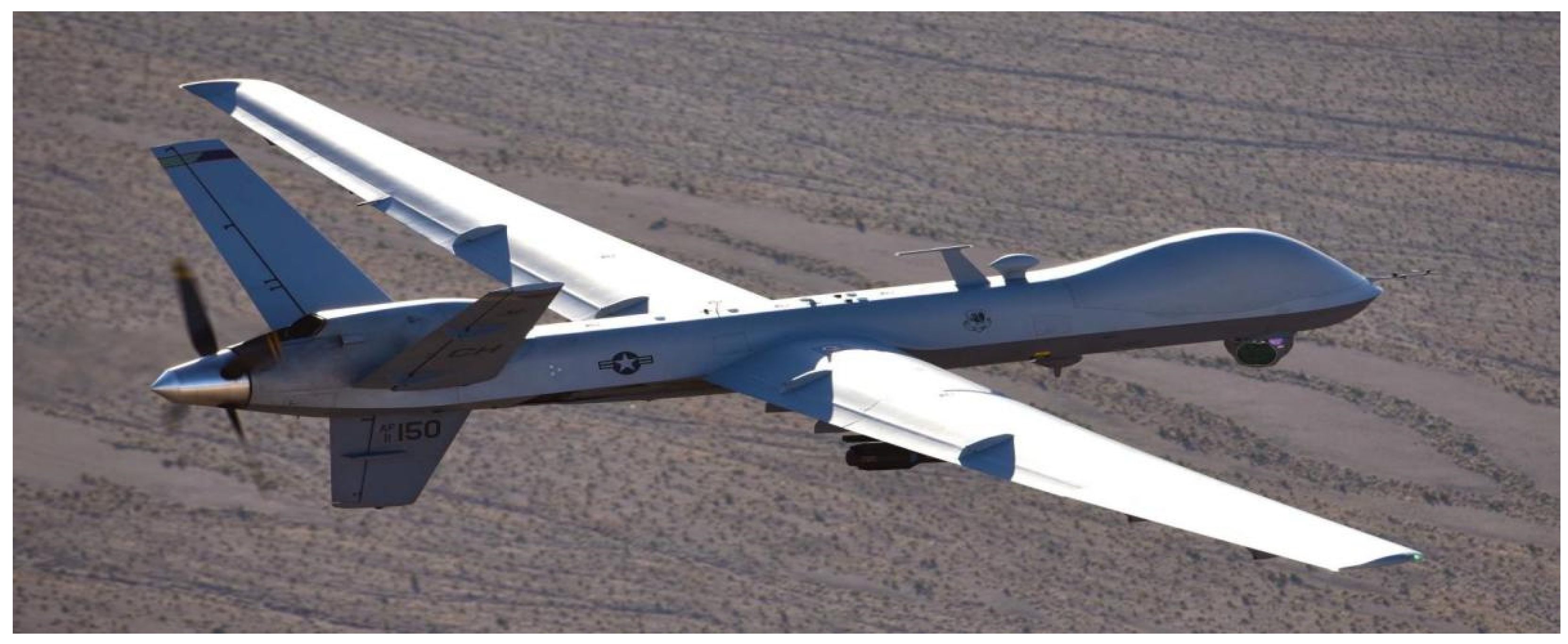
Compared with generic risk-based planners, the risk term used in this work is not an abstract heuristic or probabilistic risk field. Instead, it is a detection-margin-based soft risk cost defined only inside the hard no-detection-threshold-exceedance feasible region. The resulting contribution is therefore a unified hard-feasibility/soft-risk Risk-A*-MPC framework for low-altitude fixed-wing UAV path planning under dynamic radar-based sensing constraints.The representative fixed-wing MALE UAV considered in this study is illustrated in Figure 1.

2. Modeling

2.1. Terrain Environment Modeling

A DEM-based terrain model is adopted to represent terrain elevation, AGL constraints, and LOS occlusion in the planning process [37]. The terrain is stored as a two-dimensional grid, with interpolation used for continuous-position elevation queries. This model supports the subsequent LOS-based detection constraint and risk evaluation.

2.1.1. Two-Dimensional Discrete Terrain Grid Model

Assume that the mission area on the horizontal plane is discretized into a regular grid, where the row and column indices are denoted by r { 1 , , N r } and c { 1 , , N c } , respectively. The DEM provides the ground elevation at the center of each grid cell, denoted as Z [ r , c ] . Thus, the DEM defines a grid-based elevation field. The grid resolution s converts grid distance into physical distance [37]:
d metric = s d p x
where d p x is the distance measured in grid units, and d metric is the corresponding physical distance on the two-dimensional plane.

2.1.2. Terrain Elevation Query at Continuous Locations (Bilinear Interpolation)

In planning and simulation, UAV, start, and goal positions are represented by continuous grid coordinates ( r , c ) R 2 . Bilinear interpolation is used to query the continuous elevation field Z ^ ( r , c ) [38]. For a continuous coordinate ( r , c ) on the two-dimensional plane, let
r 0 = r , r 1 = r 0 + 1 , c 0 = c , c 1 = c 0 + 1
and define the fractional parts as α = r r 0 , β = c c 0 , α , β [ 0 , 1 ) . Here, Z r 0 , c 0 , Z r 1 , c 0 , Z r 0 , c 1 and Z r 1 , c 1 are the given terrain elevations at the four neighboring DEM grid cells surrounding ( r , c ) , and are treated as known quantities in the bilinear interpolation. The interpolated elevation is given by
Z ^ ( r , c ) = ( 1 α ) ( 1 β ) Z r 0 , c 0 + α ( 1 β ) Z r 1 , c 0 + ( 1 α ) β Z r 0 , c 1 + α β Z r 1 , c 1

2.1.3. Terrain Occlusion and LOS Determination Model

Terrain relief may block the radar-UAV LOS and reduce detectability. Thus, a UAV within geometric radar range may still be undetectable under terrain occlusion. Therefore, LOS visibility is treated as a necessary condition for radar-based detection [39].
 A. 
Three-dimensional geometric description
At a given time instant, the radar position and AGL antenna height are denoted by ( r R , c R ) and h R , respectively. The UAV horizontal position and AGL are denoted by ( r T , c T ) and h T , respectively. The corresponding altitude above sea level (ASL) is defined as
H R = Z ^ ( r R , c R ) + h R , H T = Z ^ ( r T , c T ) + h T
The horizontal interpolation point on the line segment connecting the radar and the UAV, parameterized by λ [ 0 , 1 ] , is given by r ( λ ) , c ( λ ) :
r ( λ ) = r R + λ ( r T r R ) , c ( λ ) = c R + λ ( c T c R )
The “straight-line height” (absolute altitude) of the connecting line at this point is
H l i n e ( λ ) = H R + λ H T H R
When λ = 0 , the point corresponds to the radar location with H line ( 0 ) = H R ; when λ = 1 , it corresponds to the UAV location with H line ( 1 ) = H T . For 0 < λ < 1, the point represents an intermediate position along the line segment, and its horizontal coordinate is r ( λ ) ,   c ( λ ) .
 B. 
Sampling-based determination
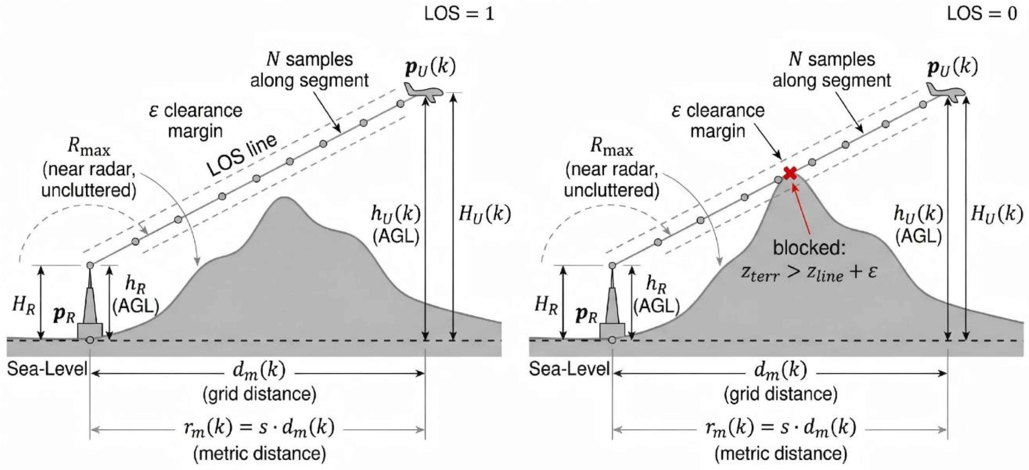
Along the segment from ( r R , c R ) to ( r T , c T ) , N points are uniformly sampled for the LOS visibility test. If there exists any sampled point satisfying
Z ^   r ( λ i ) , c ( λ i ) + ε H line ( λ i )
then the terrain is considered to intersect the line of sight (i.e., occlusion occurs and the UAV is not visible to the radar-based sensing system), and we set L O S = 0 ; otherwise, L O S = 1 (visible). Here, ϵ 0 is the LOS clearance margin used in the visibility test of Equations (7) and (8) and Figure 2.
Accordingly, the LOS determination can be summarized as
LOS = 1 , i ,   Z ^   r ( λ i ) , c ( λ i ) + ε < H line ( λ i ) 0 , i ,   Z ^   r ( λ i ) , c ( λ i ) + ε H line ( λ i )

2.2. UAV Kinematics and Constraint Modeling

A discrete-time reduced-order UAV kinematic model is used for both global planning and local MPC optimization. The model describes horizontal motion and enforces altitude constraints through ASL and AGL variables. This formulation maintains terrain clearance while limiting excessive altitude. The UAV state is updated using a discrete time step Δ t . It should be noted that the detection-threshold constraint is treated as a hard constraint in this study; that is, the planned path must first satisfy the prescribed detectability requirement before other performance indices such as total flight time are considered. In addition, because the objective of this study is planning-level and guidance-level trajectory optimization rather than high-fidelity flight-dynamics simulation, the UAV is represented by a reduced-order kinematic model that does not explicitly account for roll, pitch, or other full three-dimensional attitude dynamics [40,41]. The effects of maneuverability are instead approximated through bounded heading-rate and climb/descent-rate constraints, which provide a conservative planning-level surrogate for fixed-wing trajectory feasibility.

2.2.1. UAV State Variables

The UAV state at time t k is defined as
x k = [ r k , c k , ψ k , h k A S L , h k A G L ] T
where ( r k , c k ) denotes the row and column coordinates of the UAV in the two-dimensional grid map at time t k . ψ k is the heading angle, where h k A S L and h k A G L denote the UAV altitudes in ASL and AGL, respectively. The control input consists of heading angular velocity and climb rate:
u k = ω k ,   v z , k T
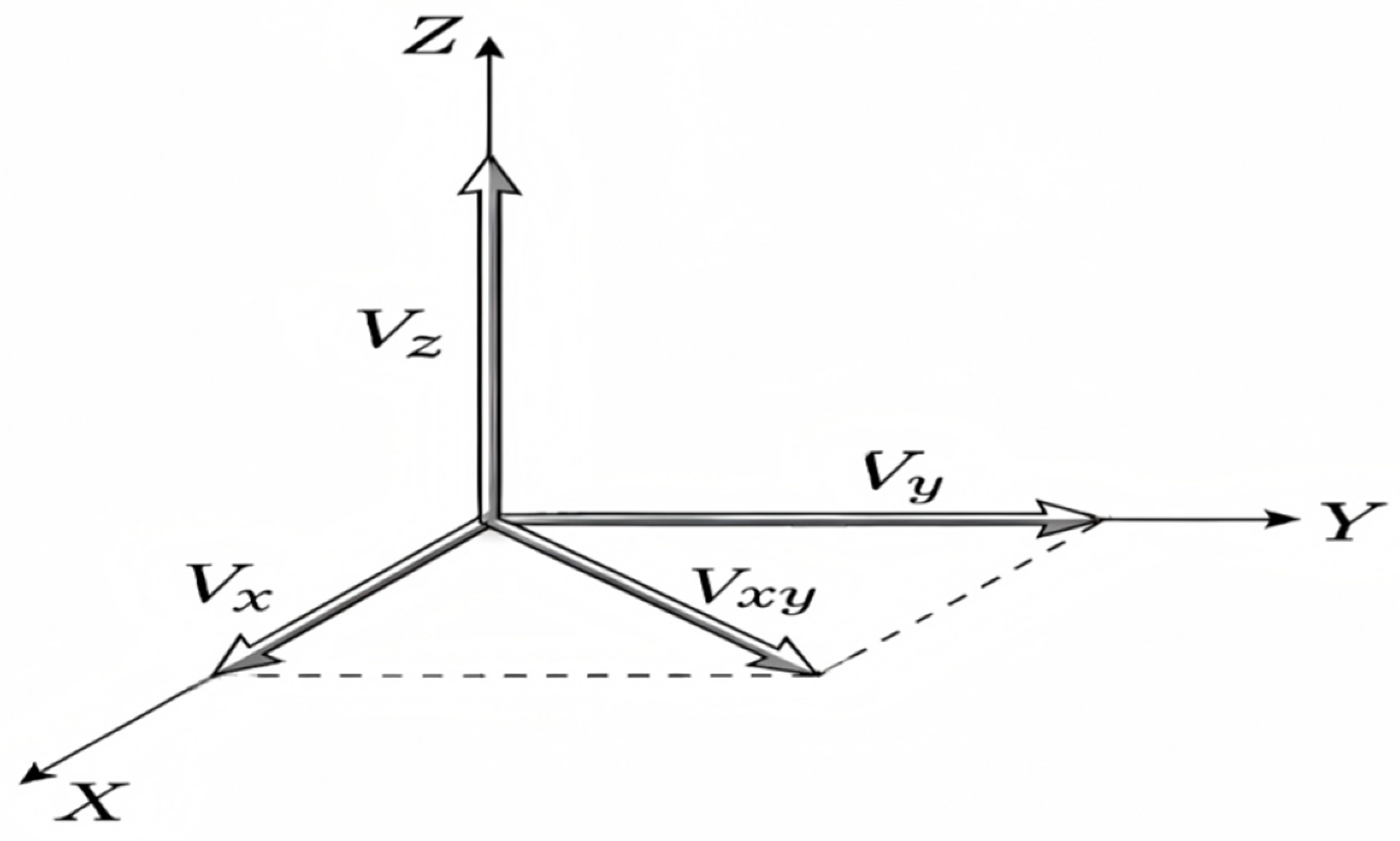
The horizontal ground-relative speed v x y is assumed constant within each time step [42,43,44].The velocity-component representation used in the kinematic model is illustrated in Figure 3.

2.2.2. Discrete-Time Planar Kinematic Model

In the grid coordinate system, the column direction can be regarded as the x-axis and the row direction as the y-axis in a discrete representation. The heading angle is updated as [45]:
ψ k + 1 = W ψ k + ω k Δ t
Here, W θ wraps the angle into π ,   π . The two-dimensional position is updated as follows:
c k + 1 = c k + v x y Δ t s cos ψ k + 1
r k + 1 = r k + v x y Δ t s sin ψ k + 1

2.2.3. Discrete-Time Vertical Motion Model and Terrain-Coupled Altitude Update

The ASL altitude is updated by integrating the climb rate:
h ˜ k + 1 ASE = h k ASE + v z , k Δ t
Because terrain elevation varies spatially, ASL and AGL are coupled through Z ^ ( · ) . Then, the predicted AGL at the next time step is:
h ˜ k + 1 AGI = h ˜ k + 1 ASE Z ^ r k + 1 ,   c k + 1
Here, h ˜ k + 1 AGI and h k + 1 AGI denote the raw and constrained AGL predictions, respectively. The terrain elevation Z ^ can be obtained via bilinear interpolation of the grid-based elevation map Z r ,   c [46]. The AGL is constrained within the allowable interval:
h k + 1 AGL = clip h ˜ k + 1 AGL ,   h min AGL ,   h max AGL
The c l i p ( ) operator enforces the lower and upper bounds [47]:
c l i p ( ξ , a , b ) = m i n ( m a x ( ξ , a ) , b )
The constrained ASL altitude is then:
h k + 1 ASI = Z ^ r k + 1 ,   c k + 1 + h k + 1 AGI
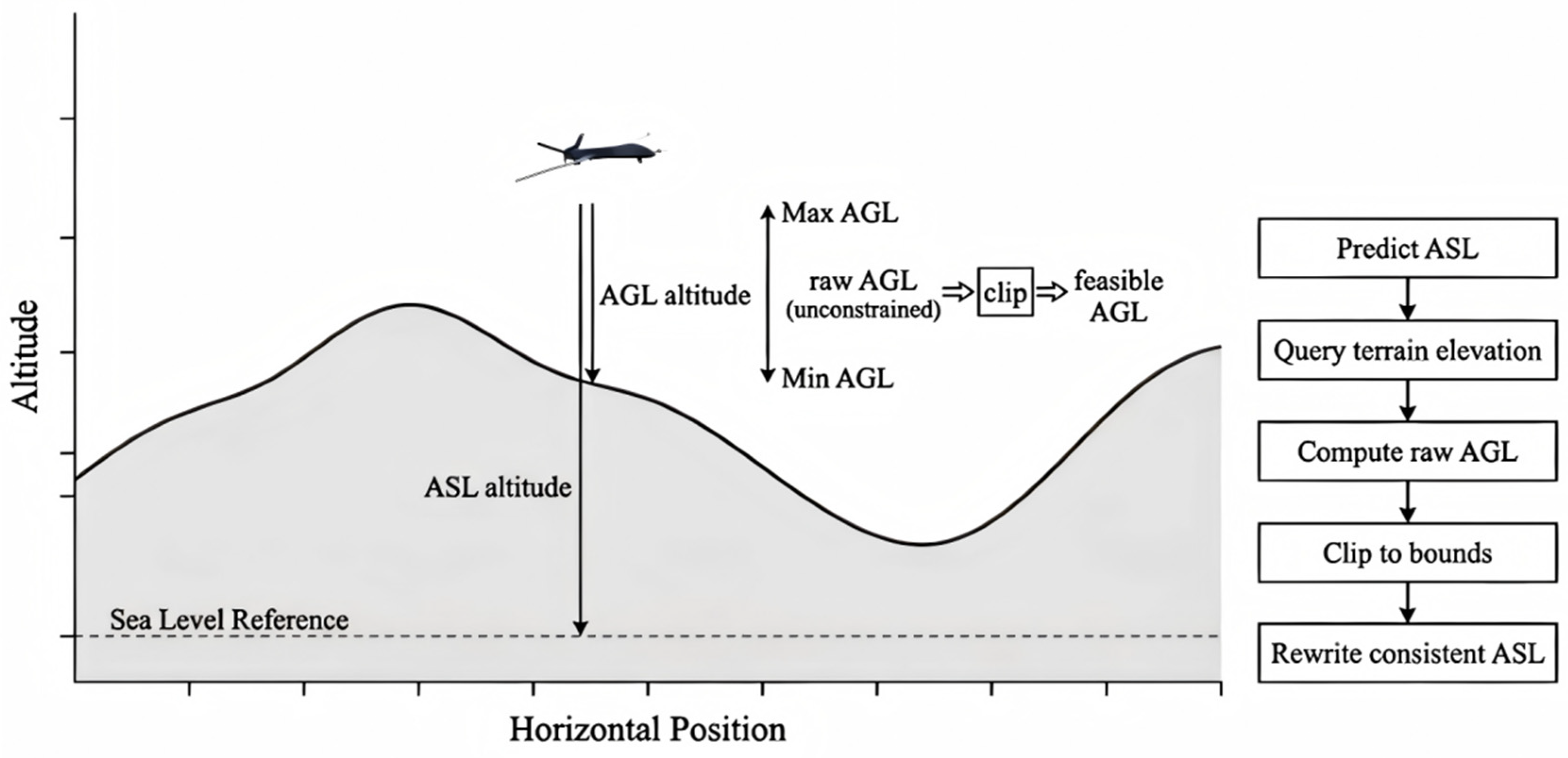
The ASL/AGL coupling and hard altitude bounds are illustrated in Figure 4.

2.2.4. Control Constraints and Feasibility Definition

The heading-rate and climb-rate constraints are imposed as follows [48]:
ω k ω max ,   v z v z , max
These bounds provide a reduced-order representation of fixed-wing maneuverability. Roll and pitch transients are not explicitly resolved in this planning-level model.

2.3. Radar Detection Model and Line-of-Sight Constraints

The sensing model considered in this section is restricted to radar-based detection. This section establishes a radar-UAV detectability model based on radar-UAV distance, LOS visibility, and maximum detection range.

2.3.1. Three-Dimensional Geometric State and Radar-Target Distance Model

We first analyze a ground-based radar deployed within the mission area. For the m = t h radar, its horizontal position in grid coordinates is denoted as
p R , m = r R , m ,   c R , m T
The antenna height is h R . Using the DEM elevation field, the radar-antenna ASL is given by
H R , m = Z ^ p R , m + h R
The UAV horizontal position at discrete time t k is
p U ( k ) = r U ( k ) ,   c U ( k ) T
The UAV altitude is constrained within the allowable interval h U ( k ) h min ,   h max . The horizontal grid distance between the radar and the UAV is defined as
d m ( k ) = p U ( k ) p R , m 2
The physical horizontal distance is
r m ( k ) = s d m ( k )
This distance is used for range gating and radar attenuation evaluation [49].

2.3.2. Line-of-Sight Visibility

Terrain occlusion may make a target undetectable even within radar coverage. The LOS state with respect to the m = t h radar is defined as a binary variable:
LOS m ( k ) = 0 not   visible 1 visible
The LOS state is obtained using the sampling-based visibility test in Section 2.1.3 [50].

2.3.3. Maximum Detection-Range Constraint

Even when LOS = 1 , radar detection is still limited by the maximum effective detection range. For the m = t h radar, if
r m ( k ) > R max
The UAV is then regarded as outside the effective radar coverage [51].

2.3.4. Detection Threshold Based on the Radar Equation

Given r m ( k ) R max and LOS m ( k ) = 1 , this paper adopts a simplified free-space radar equation to define a deterministic detection metric. Detection is declared successful when the metric exceeds a prescribed threshold [52,53]:
Metric m k = O b c N c o h P t G t G r λ 2 σ 4 π 3 r m k 4 k B T 0 B N F L
Here, P t is the radar transmit power; G t , G r are the transmit and receive antenna gains; λ is the radar wavelength; σ is the target RCS (i.e., the UAV RCS); N c o h is the effective number of coherent pulse integrations; O b c denotes the processing gain; r is the radar-to-UAV distance; k B is the Boltzmann constant; T 0 is the equivalent noise temperature; B is the receiver equivalent noise bandwidth; N F is the noise figure; and L is the overall system loss factor.
Let η denote the detection threshold. Then, the detection decision of radar m for the UAV is given by
D m ( k ) = 1 , Metric m ( k ) η 0 , Metric m ( k ) < η
The detection threshold η is calibrated at the reference boundary r = R m a x under LOS visibility by enforcing Metric R m a x ,   σ r e f = η . Here, σ r e f denotes the reference RCS used for threshold calibration. In this study, η should be interpreted as a post-processing SNR-based detection metric, because coherent integration and processing gain are already included in Equation (27). Therefore, the adopted threshold corresponds to a physically interpretable radar/SNR setting at the prescribed reference detection boundary, rather than to an arbitrary numerical cutoff.

2.3.5. Overall Detectability Determination Under Multi-Radar Fusion

When N r a d radars are present, the UAV is regarded as exposed if at least one radar satisfies the deterministic detection condition, where N r a d denotes the total number of radars and m { 1 , , N r a d } denotes the radar index. Accordingly, the overall detection event is defined as [54]:
E ( k ) = m = 1 N r a d r m ( k ) R max LOS m ( k ) = 1 M k , σ max η
Accordingly, the feasibility constraint for selecting the UAV trajectory is
ε ( k ) = 0 , k
That is, throughout the planning horizon, the UAV trajectory must never trigger the deterministic detection condition of any of the N r a d radars. To jointly represent the effects of range gating and LOS masking in the planning process, we further define the continuous-valued effective detectability M m   ( k ) of the m t h radar at time step k as
M m ( k ) = I ( r m ( k ) R max ) I ( LOS m ( k ) = 1 ) Metric m ( k )
where I ( ) denotes the indicator function.

2.4. Anisotropic RCS Modeling of the UAV

The radar-detection feasibility region is constructed using range gating, LOS hard gating, and radar-equation-based thresholding. The target RCS σ varies with the relative radar-UAV aspect angle. A simplified horizontal-plane anisotropic RCS model is therefore coupled with the heading state ψ for planning-level detectability evaluation [55,56,57].

2.4.1. Horizontal Aspect Angle and Azimuth Definition

Assume that the link between the m = t h radar and the UAV is visible, i.e., LOS = 1 . At time t k , the UAV horizontal position in grid coordinates is denoted by
p k = r k ,   c k T
with heading angle ψ k . The radar position is denoted by
p R , m = r R , m ,   c R , m T
The horizontal line-of-sight vector from the UAV to the radar is then defined as
g m , k = p R , m p k
Considering the image-like grid convention, the horizontal azimuth angle is defined as
β m , k = atan 2 ( g m , k ( r ) ,   g m , k ( c ) )
where g m , k ( r ) and g m , k ( c ) denote the row- and column-direction components of the horizontal LOS vector, respectively.
The horizontal aspect angle between the UAV heading and the radar direction is then defined as
α m , k W β m , k ψ k 0 , π
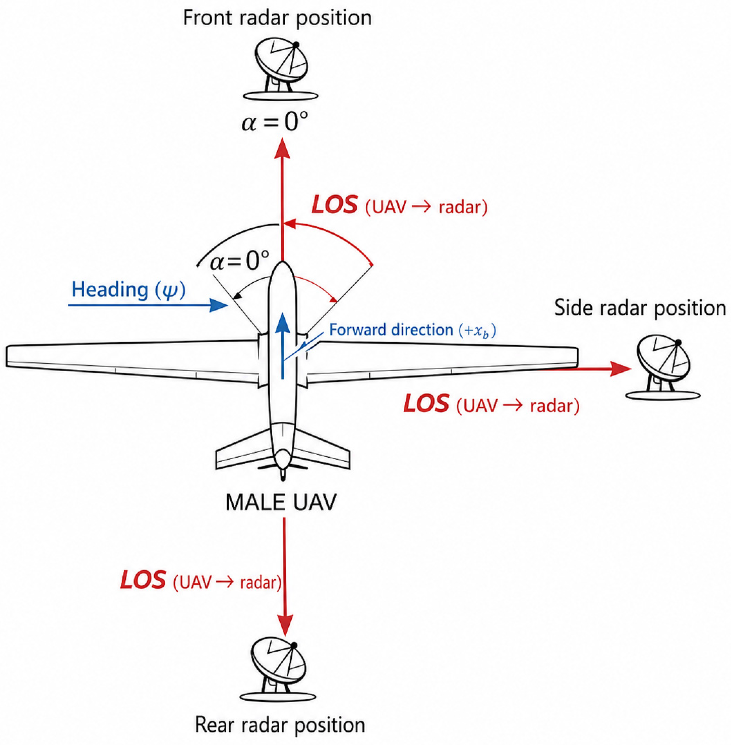
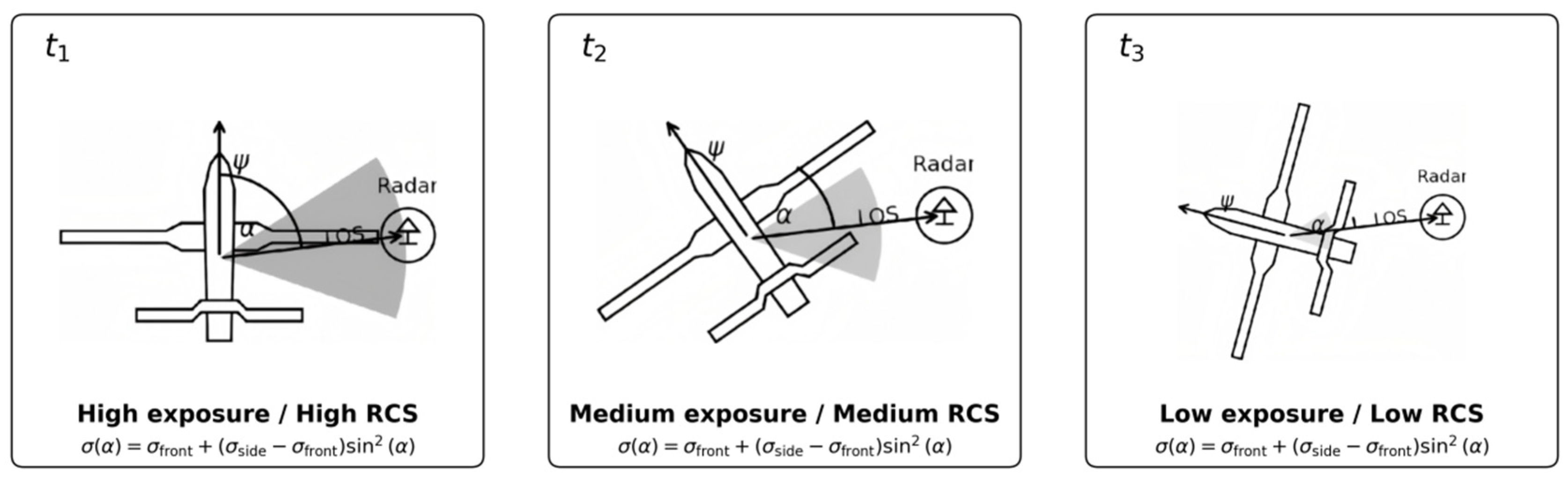
Here, α = 0 indicates that the radar is located in front of the UAV (head-on aspect), α = π 2 corresponds to a side aspect, and α = π indicates that the radar is behind the UAV (tail-on aspect) [58].

2.4.2. Parameterized Model of Anisotropic RCS

A simplified horizontal anisotropic RCS model is adopted to represent lower front/rear RCS and higher lateral RCS [36]:
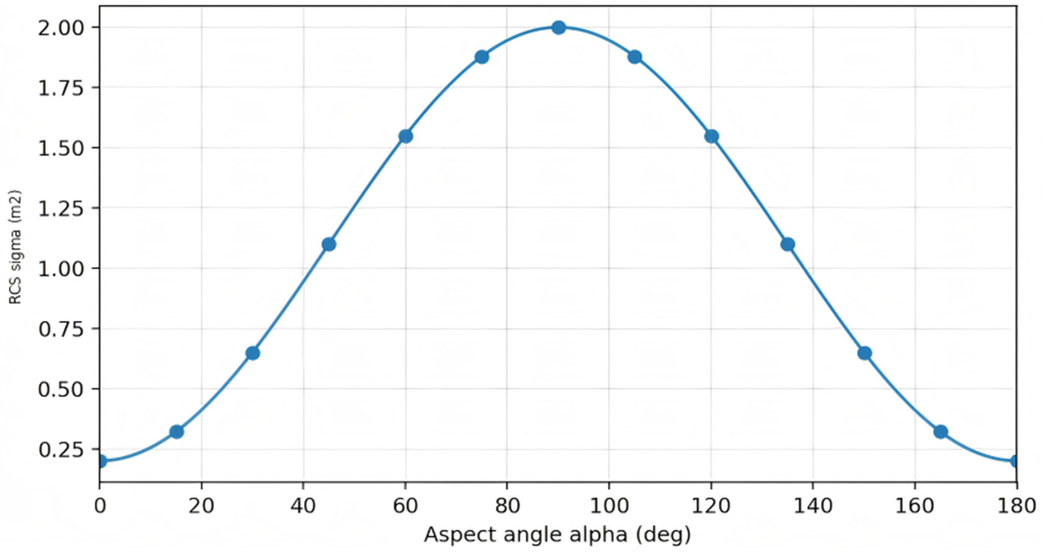
σ ( α ) = σ f r o n t + σ s i d e σ f r o n t sin 2 ( α ) , α [ 0 , π ]
where σ f r o n t denotes the effective RCS in the head-on/tail-on direction (nose/tail aspect), and σ s i d e denotes the effective lateral RCS. Accordingly,
σ ( α ) = σ f r o n t α = 0   or   π σ f r o n t α = π 2
The adopted parameterized anisotropic RCS model is illustrated in Figure 5.
This simplified model provides a continuous heading-dependent RCS term that can be directly embedded into the detectability constraint.

2.4.3. Model Assumptions

To maintain a tractable planning-level formulation, the anisotropic RCS of the UAV is assumed to vary only with the horizontal aspect angle α . Under this assumption, heading changes are used to represent the dominant planning-level coupling between trajectory direction and radar detectability, whereas RCS variations caused by three-dimensional attitude changes such as roll and pitch are not explicitly modeled. The effect of three-dimensional altitude is incorporated through LOS determination and radar-range attenuation within the detection framework. This assumption limits the proposed RCS model to heading-dependent detectability analysis and makes it unsuitable for high-fidelity characterization of roll-, pitch-, elevation-angle-, or frequency-dependent scattering effects. Therefore, the results should be interpreted as planning-level detectability estimates rather than full three-dimensional electromagnetic or flight-dynamic simulations.

3. Algorithm Framework

We assume that prior information on radar-platform locations and motion patterns is available before flight [59,60]. These data are used only to construct the planning risk field, not to model onboard interception or early-warning sensing [61,62,63,64]. The overall procedure of the proposed Risk-A*-MPC framework is summarized in Algorithm 1.
Algorithm 1: The procedure of the Risk-A*-MPC framework
Input: DEM-based terrain grid Z grid resolution s start state x 0 , goal region G g o a l , discrete altitude layers H radar-patrol prediction model, radar parameters, UAV kinematic limits, AGL bounds, detection threshold η Risk-A* weights w d and λ MPC horizon N p , control update period Δ t , finite heading-rate and climb-rate candidate sets, and objective-function weights.
Output: Executed UAV trajectory Π exec , applied control sequence U e x e c , global reference path Π g , exposure time T e x p , LOS-visible duration T L O S , and success/failure flag.
1: Load the DEM and construct the continuous terrain-elevation query Z ^ ( r , c ) by bilinear interpolation.
2: Construct the layered three-dimensional planning grid G d by combining each horizontal grid node with the admissible ASL altitude layers.
3: For each node q i in G d , compute its AGL altitude h AGL ( q i ) and mark q i as terrain-infeasible if h AGL ( q i ) h m i n ,   h m a x .
4: Predict the time-varying positions and antenna altitudes of all radar platforms over the planning interval.
5: Initialize the Risk-A* open set with the start node, set g ( q start ) = 0 , estimate t ^ ( q start ) = t 0 and initialize the closed set as empty.
6: while the open set is not empty do
7:  Select the node q i with the smallest f q i = g q i + h q i , and move q i from the open set to the closed set.
8:  if q i reaches the goal region then
9:     Backtrack the parent links to obtain the sampled global path Π d .
10:   break.
11:  end if
12:  Generate the three-dimensional neighbor set N 3 D q i using eight-connected horizontal moves and discrete altitude-layer transitions.
13:  for each neighbor q j in N 3 D q i do
14:   if q j is in the closed set or q j violates the minimum terrain-clearance constraint then
15:    continue.
16:   end if
17:   Compute the horizontal step length d x y q i , q j , altitude change Δ h , transition time Δ t ( q i , q j ) , and estimated arrival time t ^ ( q j ) .
18:   if | Δ h | > v z , max Δ t ( q i , q j ) , then
19:    Reject q j because the climb/descent-rate constraint is violated, and continue.
20:   end if
21:   For each radar m evaluate range gating, terrain-induced LOS visibility, and the conservative radar metric using σ max = σ side .
22:   Compute the node-level effective detectability M ( q j , t ^ ( q j ) ; σ max ) by taking the maximum detectability over all radars.
23:   if M ( q j , t ^ ( q j ) ; σ max ) η , then
24:    Reject q j because the no-detection-threshold-exceedance constraint is violated, and continue.
25:   end if
26:   Compute the detection margin η M ( q j , t ^ ( q j ) ; σ max ) and the soft risk cost c risk ( q j , t ^ ( q j ) ) .
27:   Update the tentative accumulated cost g tent = g ( q i ) + w d d ( q i , q j ) + λ c risk ( q j , t ^ ( q j ) ) .
28:   if q j is not in the open set or g tent < g ( q j ) , then
29:    Set parent ( q j ) = q i , g ( q j ) = g tent and f q j = g q j + h q j .
30:    Insert or update q j in the open set.
31:   end if
32:  end for
33: end while
34: if no sampled global path Π d is found then
35:  Return failure.
36: end if
37: Map Π d to continuous coordinates and resample it by arc length to obtain the equally spaced global reference path Π g .
38: Initialize the current UAV state x k x 0 , the applied control sequence U exec , the executed trajectory Π exec { x 0 } , and the safety statistics T exp 0 and T LOS 0 .
39: while x k has not reached the goal region do
40:  Update the predicted radar positions over the MPC horizon according to the radar-patrol prediction model.
41:  Select the look-ahead point p k la on Π g as the local tracking target.
42:  Construct the finite set of candidate rollouts using the piecewise-constant heading-rate and climb-rate candidates over the horizon N p .
43:  if stall detection is activated then
44:   Use the enlarged finite-control candidate grid for recovery planning.
45:  end if
46:  Set the best feasible rollout cost J best + and the best rollout U best .
47:  for each candidate rollout U cand do
48:   Propagate the predicted state sequence using the discrete-time UAV kinematic model.
49:   Set feasible = true and J = 0 .
50:   for each prediction step j = 0 , , N p 1 do
51:    Check the control bounds, AGL bounds, and terrain-coupled altitude update.
52:     For each radar m compute the LOS azimuth, heading-dependent aspect angle, dynamic RCS σ m , k + j , range gating, and terrain-induced LOS visibility.
53:    Compute the radar-specific detectability M m ( k + j ) and the fused detectability M ( k + j ) = max m M m ( k + j )
54:    if M k + j η or any kinematic/AGL constraint is violated then
55:     Set feasible = false and stop evaluating this rollout.
56:    end if
57:    Accumulate the tracking cost, control-smoothing cost, detection-margin-based soft risk cost, and terminal progress cost.
58:   end for
59:   if feasible = true and J < J best , then
60:    Set J best J and U best U cand .
61:   end if
62:  end for
63:  if U best = , then
64:   Mark the MPC update as infeasible and return failure for the current rollout.
65:  end if
66:  Set u k first ( U best ) and apply u k to the UAV.
67:  Update the actual UAV state x k + 1 , append the applied input to U e x e c , and append x k + 1 to Π exec .
68:  Evaluate the executed state using the same range-gating, LOS, radar-equation thresholding, and exposure-time rules.
69:  Update T e x p and T L O S , set k k + 1 , and repeat the receding-horizon optimization.
70: end while
71: Return Π exec , U e x e c , Π g , T e x p , T L O S and the success flag, success = true.

3.1. Risk-A* Algorithm

3.1.1. Construction of the Three-Dimensional Spatio-Temporal Risk Map

Global planning is performed on a sampled grid G α . The two-dimensional planning space is extended into a layered three-dimensional grid. For each horizontal grid node C i corresponding to the two-dimensional coordinate x i ,   y i T , a discrete altitude set H = h ( 1 ) , , h ( L ) is introduced, and the three-dimensional node is defined as
q i ( c i , h ( l ) )
Here, h ( l ) denotes the ASL. The terrain elevation is provided by the DEM and denoted as Z ^ ( p ) , where p i = x i ,   y i T is the horizontal position corresponding to node q i . The spatio-temporal risk map is then constructed by combining terrain feasibility, dynamic feasibility, and radar-detection feasibility on the above three-dimensional node set.
 A. 
Terrain avoidance and dynamic feasibility hard constraints
Terrain safety constraints are imposed as follows:
(1) Minimum ground-clearance constraint
The altitude above ground level is defined as
h AGI ( q i ) h ( l ) Z ^ ( p i )
Given the minimum safe ground-clearance margin h min , the terrain-collision forbidden region is defined as
occ t e r ( q i ) = I h A G L ( q i ) < h min
(2) Feasibility constraints on climb/descent rate
For a neighboring transition q i q j , let the horizontal step length be d x y ( q i , q j ) = p j p i 2 and the altitude change be Δ h = h j h i . Using the prescribed horizontal speed v x y , the time increment associated with this step is estimated as
Δ t ( q i , q j ) d x y ( q i , q j ) v x y
Using the climb/descent rate bound in Equation (19), the climb-rate-infeasible region is
occ c l i m b ( q i , q j ) = I | Δ h | Δ t ( q i , q j ) > v z , max
Equations (40)–(43) define the terrain and Δ t ( q i , q j ) d x y ( q i , q j ) v x y kinematic hard-feasibility conditions.
 B. 
Spatio-temporal radar risk and continuous risk cost
A discrete-time sequence is used to represent time-varying radar geometry:
t k = k Δ t
At each time t k , the m-th radar occupies a predicted horizontal position denoted by
p R , m ( t k ) = r R , m ( t k ) c R , m ( t k )
According to Equation (21), the corresponding radar-antenna absolute altitude is
H R , m = Z ^ ( p R , m ) + h R
For a three-dimensional node q i , the target absolute altitude is directly given by h ( l ) . Therefore, the geometric quantities required for radar detection can be evaluated at the node level. First, the horizontal grid distance between node q i and radar m at time t k is computed as [65]
d m ( k ) = p U ( k ) p R , m 2
r m ( q i , t k ) = s p i p R , m ( t k ) 2
where s is the grid resolution (unit: m/px), consistent with Equation (24). Using the terrain-occlusion test in Section 2.1.3, the LOS state is written as
LOS ( q i , t k ) = LOS ( p R , m ( t k ) , p i , H R , m ( t k ) , h ( l ) ) { 0 , 1 }
In the global layer, the future heading of the UAV has not yet been optimized, and thus the exact instantaneous anisotropic RCS is unknown. To construct a conservative safe corridor, the worst-case upper bound of the heading-dependent RCS is adopted. From Equation (37), σ ( α ) σ side for all α [ 0 , π ] . Therefore, we set σ max = σ side in the global planner. Moreover, for fixed q i , t k , range gating, and LOS state, the radar metric in Equation (27) is monotonically increasing with respect to σ . Hence,
Metric m ( q i , t k ; σ ( α ) ) Metric m ( q i , t k ; σ max )
which implies that the forbidden region generated by σ max is a conservative outer approximation of the true exposed region. Substituting r m q i , t k and σ max into the radar equation in Equation (27) yields the conservative radar metric Metric m ( q i , t k ; σ max ) . Accordingly, the effective detectability contributed by radar m is defined as
M m ( q i , t k ; σ max ) = I [ r m ( q i , t k ; σ max ) R max ] I [ LOS m ( q i , t k ) = 1 ] Metric m ( q i , t k ; σ max )
Equation (49) combines range gating, LOS hard gating, and radar-equation-based thresholding at each graph node.
In a multi-radar environment, the radar with the maximum effective detectability is taken as the overall effective detectability at node q i
M ( q i , t k ; σ max ) = max m M m ( q i , t k ; σ max )
Given the detection threshold η , the detection-threshold-exceedance forbidden-state indicator at time t k is defined as
occ rad ( q i , t k ) = I [ M ( q i , t k ; σ max ) η ]
Within the feasible region where occ rad ( q i , t k ) = 0 , to distinguish nodes close to the detection boundary from those far away from it, a detection margin is introduced:
margin ( q i , t k ) = η M ( q i , t k ; σ max )
A smaller margin indicates higher detection risk. Based on this margin, a continuous risk cost c risk is constructed to evaluate the safety level of a given region:
c risk ( q i , t k ) = exp margin ( q i , t k ) κ
Here, κ controls the decay rate of the risk penalty [66].
 C. 
Unified Representation of Hard Feasibility and Soft Cost in the Three-Dimensional Grid
The final spatio-temporal forbidden-state indicator in the three-dimensional grid is defined as
occ ( q i , t k ) = occ ter ( q i ) occ rad ( q i , t k )
In the region where occ ( q i , t k ) = 0 , the continuous cost c risk is used as a soft penalty to steer the global path away from high-risk areas. Although the general idea of combining hard feasibility constraints with soft costs is commonly adopted in risk-aware planning problems, the formulation used here is specifically constructed as a spatio-temporal radar-detection feasibility map in which terrain clearance, climb-rate feasibility, LOS/range-gated radar exposure, conservative worst-case RCS, and a detection-margin-based continuous risk cost are evaluated jointly at each three-dimensional graph node.

3.1.2. Three-Dimensional Risk-A* Search

Risk-A* search is performed on the above three-dimensional spatio-temporal risk map. The evaluation function for node q i is defined as
f q i = g q i + h q i
where g q i denotes the accumulated cost and h q i denotes the heuristic estimated cost-to-go.
 A. 
State definition and neighborhood expansion
Each search state is directly represented by the three-dimensional node q i defined in Equation (39). To account for time-varying risk, an estimated arrival time t ^ ( q i ) is maintained for each node. Neighbor expansion is performed using “eight-connected neighbors in the horizontal plane + discrete altitude-layer transitions”, and the neighbor set is denoted by N 3 D q i . For any neighbor q j N 3 D ( q i ) , let the horizontal step length be d x y ( q i , q j ) = p j p i 2 , and let the altitude change be Δ h = h j h i . The geometric step length is computed as
d ( q i , q j ) = d x y 2 ( q i , q j ) + ( Δ h ) 2
The arrival time is propagated as
t ^ ( q j ) = t ^ ( q i ) + Δ t ( q i , q j ) , Δ t ( q i , q j ) d x y ( q i , q j ) v x y
where the approximation follows from the prescribed constant horizontal speed v x y adopted in the global layer.
 B. 
Triple-pruning based on terrain avoidance, dynamic feasibility, and radar hard feasibility
For each candidate expansion q i q j , pruning is applied in the following order:
(1) Terrain-collision pruning: if occ ter ( q j ) = 1 , the node violates the minimum terrain-clearance requirement and is discarded.
(2) Dynamic-feasibility pruning: if occ climb ( q i , q j ) = 1 , the transition exceeds the climb/descent rate bound and is discarded.
(3) Detection-threshold hard-feasibility pruning: the detection-threshold violation indicator is evaluated for the candidate node q j at its estimated arrival time t ^ ( q j ) as
occ rad ( q j , t ^ ( q j ) ) = I [ M ( q j , t ^ ( q j ) ; σ max ) η ]
If occ rad ( q j , t ^ ( q j ) ) = 1 , the node is considered exposed and thus infeasible; otherwise, it is admissible. This pruning ensures that only terrain-safe, dynamically feasible, and detection-feasible nodes enter the open set.
 C. 
Cost function: path length + soft risk penalty
For an admissible expansion, the accumulated cost at the estimated arrival time t ^ ( q j ) is updated as
g ( q j ) = g ( q i ) + w d d ( q i , q j ) + λ c risk ( q j , t ^ ( q j ) )
Here, w d is the weight for path length, and λ is the risk weight. The soft risk cost c risk is defined in Equation (53) and penalizes states closer to the detection boundary within the feasible region.
The heuristic function adopts the lower bound of the three-dimensional Euclidean distance:
h ( q i ) = w d s p i p goal 2 2 + h i h goal 2
 D. 
Output of the reference path
After the search is completed, the sampled three-dimensional path is obtained as
Π d = q 0 , q 1 , , q N p a t h
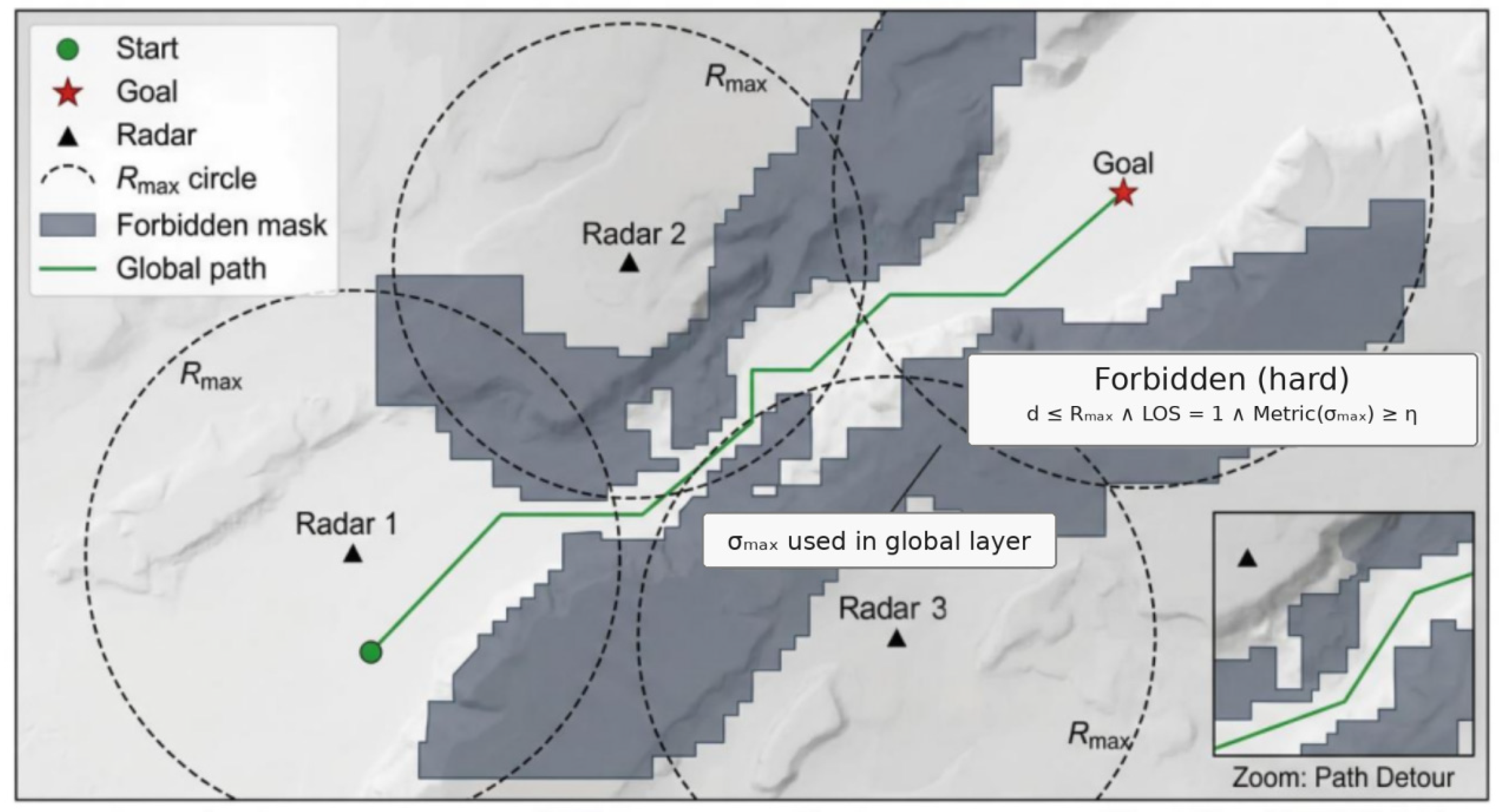
where N p a t h denotes the terminal-node index of the sampled global path. The discrete path is mapped to continuous coordinates and resampled to generate the MPC reference path Π g .The generated MPC reference path is illustrated in Figure 6.

3.2. Risk-Constrained Receding-Horizon MPC for Local Planning

The Risk-A* algorithm produces a low-risk reference path Π g on the spatio-temporal risk map defined over the sampled grid G d . The MPC algorithm performs local planning at each discrete time step using a receding-horizon model [67]. While tracking Π g , it enforces the same detection-threshold constraint defined in Section 3.1. Unlike the conservative global layer, the MPC layer embeds the heading-dependent RCS term into the receding-horizon detectability constraint while optimizing trajectory tracking, smoothness, and detection margin.The dynamic RCS modulation mechanism used by the MPC layer is illustrated in Figure 7. In Figure 7, the shaded sector represents the qualitative radar-illuminated exposure region associated with the current radar-UAV LOS; it is used only to visualize the relative effective detectability caused by the aspect-angle-dependent RCS, rather than to denote an additional radar-beam model.

3.2.1. Prediction Model

At the current time t k , the local MPC layer optimizes the predicted state sequence x k + j j = 0 N p and control sequence u k + j j = 0 N p 1 over a prediction horizon of length N p . Here, N p denotes the MPC prediction horizon length, subject to the system dynamics
min u k + j j = 0 N p 1 J , s . t . x k + j + 1 = f x k + j , u k + j , j = 0 , , N p 1
Here, the state vector and control input are defined consistently with Equations (9) and (10), i.e., x k + j = r k + j , c k + j , ψ k + j , h k + j A S L , h k + j A G L T and u k + j = ω k + j , v z , k + j T . Using the same constant horizontal ground-relative speed v x y , the discrete-time prediction model is explicitly written as
ψ k + j + 1 = W ψ k + j + ω k + j Δ t c k + j + 1 = c k + j + v x y Δ t cos ψ k + j + 1 r k + j + 1 = r k + j + v x y Δ t sin ψ k + j + 1 h ˜ k + j + 1 A S L = h k + j A S L + v z , k + j Δ t h ˜ k + j + 1 A G L = h ˜ k + j + 1 A S L Z ^ r k + j + 1 , c k + j + 1 h k + j + 1 A G L = clip h ˜ k + j + 1 A G L , h min , h max
The control and altitude bounds are enforced as
ω k + j ω max , v z , k + j v z , max , h min h k + j A G L h max , j = 0 , , N p 1
The time discretization is consistent with Equation (44), namely t k + j = ( k + j ) Δ t .

3.2.2. Effective Detectability

Let the predicted UAV horizontal position at step k + j be p k + j = r k + j , c k + j . For the m-th radar, its predicted horizontal position at time t k + j is p R , m ( t k + j ) , consistent with Equation (45). Following Section 2.4.1 and using the unified angle-wrapping operator W ( ) , the horizontal line-of-sight vector, azimuth angle, aspect angle, and dynamic RCS are given by
g m , k + j = p R , m ( t k + j ) p k + j β m , k + j = atan   2 g m , k + j ( r ) , g m , k + j ( c ) α m , k + j = W   β m , k + j ψ k + j [ 0 , π ] σ m , k + j = σ front + σ side σ front sin 2   α m , k + j
Meanwhile, the radar-UAV horizontal distance and LOS visibility at step k + j are evaluated as
r m ( k + j ) = s p k + j p R , m ( t k + j ) 2
LOS m ( k + j ) = LOS ( p R , m ( t k + j ) , p k + j , H R , m ( t k + j ) , h k + j A S L ) { 0 , 1 }
Substituting r m ( k + j ) and σ m , k + j into Equation (27), the effective detectability of the m-th radar is defined as
M m ( k + j ) = I [ r m ( k + j ) R max ] I [ LOS m ( k + j ) = 1 ] Metric ( k + j )
Under multi-radar fusion, the overall effective detectability is taken as the maximum among all radars:
M ( k + j ) = max m M m ( k + j )

3.2.3. Hard Safety Constraint

Within the prediction horizon, the MPC algorithm performs the same deterministic detection-threshold test as in Section 3.1, but now using the heading-dependent dynamic RCS in Equation (65). The hard safety constraint is therefore imposed as
M k + j < η , j = 0 , , N p 1
This constraint guarantees that the refined local trajectory remains entirely within the no detection-threshold-exceedance feasible region throughout the prediction horizon.

3.2.4. Soft Risk Cost and Objective Function

Based on the risk-aware reference path Π g generated by the Risk-A* algorithm, the local layer employs a receding-horizon MPC scheme to generate executable control inputs at each control cycle. To ensure consistency between global guidance and local refinement, at time t k a look-ahead point P k l α is selected along the reference path Π g as the local tracking target. Subsequently, the control sequence within the prediction horizon is optimized to balance path tracking performance, control smoothness, risk margin, and progression efficiency. The objective function is defined as
J = j = 0 N p 1 J trk k + j + J sm k + j + J risk k + j + J term k + N p
(1)
Tracking term J trk
J trk ( k + j ) = w trk p k + j p k la 2 + w alt ( h k + j AGL h ref ) 2
The horizontal tracking error is defined by the Euclidean distance between the predicted position p k + j and the look-ahead point p k la . Meanwhile, altitude regulation is imposed via the AGL term, where h k + j AGL is the altitude above ground level and h ref is the desired ground-clearance altitude.
(2)
Smoothing term J sm
J sm ( k + j ) = w ω ω k + j 2 + w v v z , k + j 2 + w Δ u u k + j u k + j 1 2
Here, u k + j = ω k + j , v z , k + j T , and u k + j u k + j 1 2 2 penalize control-rate variations to encourage smooth maneuvers. The terms w ω ω k + j 2 and w v v z , k + j 2 penalize control effort, which is related to maneuver intensity and energy consumption. For j = 0 , u k 1 denotes the control input applied in the previous control cycle.
(3)
Risk term J risk
To preserve consistency with the soft-risk design in Section 3.1.1, we introduce a detection margin based on the effective detectability M ( k + j ) defined in Section 3.2.2:
margin ( k + j ) = η M ( k + j )
A risk-shaping function is then defined as
ϕ ( margin + ( k + j ) ) = exp margin + ( k + j ) κ
Accordingly, the risk cost becomes
J risk ( k + j ) = β ϕ ( margin + ( k + j ) )
Here, β > 0 is the risk weight, and κ controls the shape and effective width of the soft risk band.
(4)
Progress term J term
To avoid loitering and inefficient oscillatory behaviors during flight, a terminal progress term is introduced:
J term k + N p = w goal p k + N p p k + N p l a 2 2 + w stall I p k + N p p k 2 < θ
Here, p k + N p p k + N p l a 2 2 denotes the distance from the predicted terminal position to the corresponding look-ahead/goal point, and the condition p k + N p p k 2 < θ penalizes insufficient net progress over the prediction horizon, thereby preventing the UAV from circling in place or moving inefficiently.

3.2.5. Numerical Implementation and Constraint Handling of the Finite-Control-Set MPC

The local receding-horizon planner was implemented as a finite-control-set rollout MPC rather than as a gradient-based nonlinear programming solver. At each control cycle, a finite set of candidate control rollouts is generated over the prediction horizon, the UAV state is propagated using the prediction model in Section 3.2.1, and the objective function in Equations (72)–(77) is evaluated only for rollouts that satisfy the feasibility tests. The first control input of the feasible rollout with the minimum cost is then applied, and the optimization is repeated at the next control cycle.
Because the online MPC problem is solved by deterministic rollout enumeration over a finite candidate set, no SQP, interior-point, IPOPT, or fmincon-type iterative nonlinear programming solver is used. As reported in Section 4.1.2, each MPC update evaluates 2025 candidate rollouts in the normal planning mode or 4225 candidate rollouts when the stall-detection mode is activated. Therefore, each online MPC update terminates after a finite number of rollout evaluations, and convergence in the sense of an iterative nonlinear-programming solver is not applicable to the online MPC layer. The effective numerical optimization settings are instead determined by the prediction horizon, the two-segment piecewise-constant control parameterization, the finite heading-rate and climb/descent-rate grids, and the hard rejection of infeasible rollouts.
The prediction horizon is denoted by N p . In the implementation used in the simulation experiments, N p = 12 and Δ t = 3   s , which corresponds to a 36 s prediction window. The horizon is divided into two piecewise-constant control segments, with N 1 = 6 and N 2 = 6 . The heading angular-rate candidates are uniformly sampled within [ ω max , ω max ] , and the climb/descent-rate candidates are uniformly sampled within [ v z , max , v z , max ] . Therefore, the control bounds are enforced directly through the candidate control sets before trajectory propagation.
At each prediction step, the terrain-coupled altitude update is checked against the prescribed AGL bounds. The detection-threshold constraint is treated as a hard feasibility condition. Specifically, if a predicted state in a rollout satisfies range gating, LOS visibility, and detection-threshold exceedance for any radar, i.e., r m ( k + j ) R max , LOS m ( k + j ) = 1 , and M m ( k + j ) η , the corresponding rollout is regarded as infeasible and excluded from the minimization. The soft risk term in Equation (76) is used only to improve the detection margin among feasible rollouts and is not used to relax the hard detection-threshold constraint.
If no feasible rollout exists within the finite candidate set at a given control cycle, the MPC update is marked as infeasible rather than being treated as a relaxed feasible solution. This all-infeasible case is used only as a numerical diagnostic for implementation robustness and does not redefine the no-detection-threshold-exceedance feasible set. In the performance evaluation, the same infeasibility-handling and exposure-evaluation rule is applied to all compared methods: safety is assessed on the actually executed trajectory using the same range-gating, LOS, and radar-equation threshold tests, so that nonzero exposure time indicates loss of local safety feasibility under the common MPC executor rather than a difference in detection modeling or evaluation criteria.

4. Simulation Experiments

4.1. Simulation Environment

This section presents the parameter settings of the overall experiment. The simulation scenario is constructed on a grid-based terrain derived from a DEM. The terrain elevation at continuous positions is obtained via interpolation, and radar-target LOS determination is incorporated so that range gating + LOS hard gating + detection thresholding are considered in a unified manner.

4.1.1. Terrain Data and Grid Configuration

(1)
Terrain source and loading
To clarify the experimental design, the simulation experiments are organized as a sequential test plan rather than as independent demonstrations of unrelated effects. First, the simulation environment, including the DEM-based terrain, UAV kinematic parameters, radar-patrol settings, detection-threshold model, and MPC implementation settings, is defined to ensure that all methods are evaluated under the same terrain, sensing, and dynamic constraints. Second, the main comparative experiments are conducted in two DEM-based mountainous terrain zones, each with one nominal start-goal pair, to evaluate whether the proposed Risk-A*-MPC framework can maintain detection-threshold feasibility when compared with baseline global reference planners combined with the same local MPC executor. Third, the ablation study is used to examine the respective contributions of the global Risk-A* layer and the local MPC layer. Fourth, the dynamic RCS analysis is included to explain the mechanism by which heading-dependent RCS modulation affects the effective detectability during LOS-visible intervals. Finally, the UAV-speed and radar-speed experiments are treated as parameter-sensitivity checks, rather than as additional primary performance claims. Therefore, the subsequent experiments are intended to support the interpretation, mechanism analysis, and robustness assessment of the main comparative results.
The simulated terrain is generated in MATLAB R2023b using publicly available satellite elevation datasets in GeoTIFF format. The DEM is read and converted into a two-dimensional grid elevation matrix Z r , c .
(2)
Grid resolution and map scale
The grid resolution is denoted by s (unit: m/px), obtained from the public DEM dataset. The map dimensions are n r and n c in the row and column directions, respectively. Horizontal positions are uniformly represented in row/column (row/col) coordinates. Physical distances are converted according to Equation (1): d metric = s d px . Here, d px denotes the pixel distance between two points in the grid map (in pixels), and d metric denotes the corresponding real-world distance (in meters). The grid resolution s represents the physical length corresponding to one pixel in the real world (unit: m/px). In this study, we set s = 30 .
(3)
Terrain visualization and downsampling
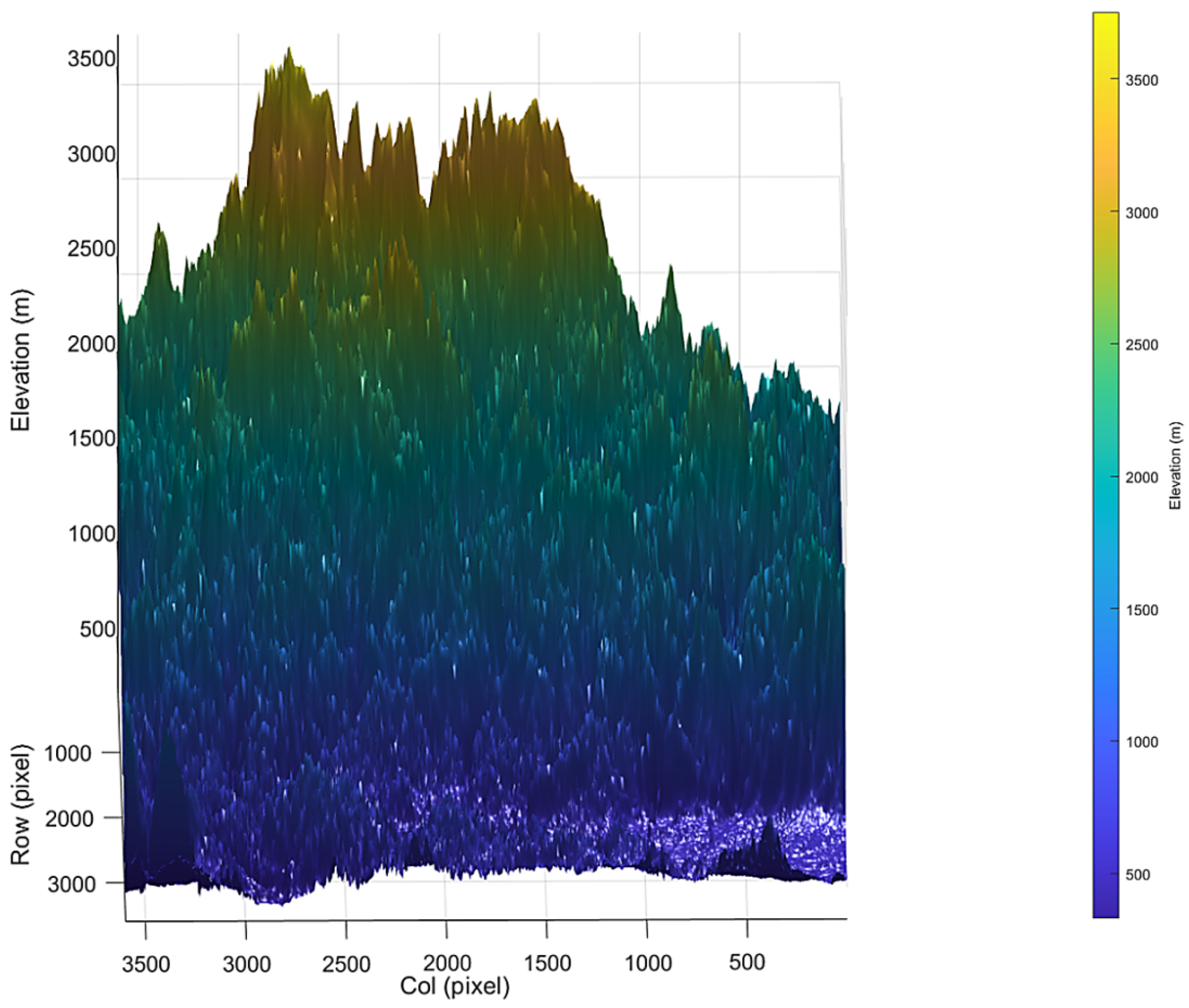
To reduce rendering overhead, the three-dimensional terrain visualization uses a uniformly downsampled grid for surface rendering, while planning and control are performed at the original resolution. Two DEM-based mountainous terrain zones are used in the simulations. The public datasets are used to generate the two terrain zones, and Figure 8 illustrates one representative generated terrain zone. The public dataset [68] is used to generate the terrain shown below.

4.1.2. Platform Parameters

(1)
UAV Parameters and Dynamic Limits
The UAV is modeled using the ground-relative planar motion with controllable turning and climb/descent introduced in Section 2.2. Within each control interval Δ t , the control inputs are the heading angular rate ω and the vertical velocity v z , while the horizontal ground-relative speed v x y is assumed to remain constant.
Following the parameter settings commonly adopted in related literature [69,70], the MPC control update period is set to Δ t = 3   s . The constant horizontal ground-relative speed is set to v x y = 600   km / h . The maximum heading angular rate is set to ω max = 25 ° / s and the maximum climb/descent rate is set to v z , max = 8   m / s . To satisfy both terrain-safety requirements and low-altitude flight requirements, the allowable AGL is constrained to h AGL 35   m , 250   m .
Consistent with the finite-control-set MPC implementation described in Section 3.2.5, the local MPC prediction horizon was set to N p = 12 , corresponding to a 36 s prediction window under the 3 s control update period. The horizon was divided into two piecewise-constant control segments, with N 1 = 6 and N 2 = 6 . In the normal planning mode, 2025 candidate rollouts were evaluated at each MPC update, whereas 4225 candidate rollouts were evaluated when the stall-detection mode was activated. The reference AGL altitude in the local altitude-regulation cost was set to 80 m.
(2)
Analysis of UAV Anisotropic RCS Characteristics
A MALE fixed-wing UAV is selected as the study platform. Here, the MALE platform is adopted to reflect its endurance and medium-altitude operational characteristics, rather than superior agility. Such UAVs typically feature a slender fuselage, high-aspect-ratio main wings, and tail structures, and may carry application-specific payloads, such as optical sensing modules, beneath the fuselage. This geometric configuration leads to significant variation in effective projected area and electromagnetic scattering characteristics under different observation aspects. When the radar is located at the lateral side of the UAV, the projected area is largest, resulting in a higher RCS-dependent detectability metric. In contrast, when the radar is positioned in the front or rear direction, the projected area is smaller and the corresponding detectability metric is reduced. To more realistically reflect the influence of UAV attitude on detectability in path planning and risk assessment, an anisotropic RCS model is adopted. The UAV RCS is modeled as a function of the horizontal aspect angle α , defined as the angle between the UAV heading and the horizontal LOS direction from the UAV to the radar. The aspect angle satisfies α 0 , π . The RCS variation with respect to aspect angle is modeled as
σ ( α ) = σ front + ( σ side σ front ) sin 2 ( α ) , α [ 0 , π ]
Here, σ front denotes the minimum scattering level when the radar is located in the front or rear direction of the UAV, and σ side denotes the maximum scattering level when the radar is located laterally. This model ensures that σ ( α ) attains its minimum at α = 0 ° and 180 ° , and reaches its maximum at α = 90 ° , exhibiting a single-peaked symmetric variation about 90 ° . By incorporating σ ( α ) into the radar detection metric, a coupling constraint among heading-RCS-detectability is established. As a result, the UAV can not only exploit terrain masking to satisfy detection-threshold constraints but also actively adjust its heading or maneuver state to avoid high-RCS sectors and reduce the detectability metric during trajectory optimization [71,72].The resulting RCS–aspect-angle relationship is shown in Figure 9.
(3)
Parameters of the ground mobile radar platform
In the experiments, the radar-sensing-constrained environment is configured with K = 3 ground mobile radar sensing platforms governed by a randomized waypoint-based patrol-motion model. For each repeated trial, one trial-specific radar-motion realization is generated from this model, and the resulting time-varying radar trajectories are supplied identically to all compared methods within that trial. Unless otherwise specified in the radar-speed robustness analysis, the ground speed of each mobile radar platform is fixed at v r a d = 8   m / s , and the radar antenna height above ground is fixed at h rad = 15   m . In the LOS test, the “radar-antenna absolute altitude-UAV absolute altitude” line segment is sampled and compared with the terrain surface samples, so that terrain occlusion is treated as a necessary condition for detection (hard gating). In the simulation, the maximum radar detection radius is set to R max = 40   k m . The detection threshold is calibrated by enforcing Metric ( R max , σ r e f ) = η [73,74,75] under LOS visibility and the adopted nominal radar/SNR setting according to Equation (27). This calibration yields η = 7132 , which is used as the deterministic planning-level detection threshold in the subsequent simulations.

4.2. Comparative Experiments

To clarify the experimental scope, this study evaluates two DEM-based mountainous terrain zones for simulation-based comparison. Terrain Zone 1 is generated from ASTGTMV003_N39W106 and Terrain Zone 2 is generated from ASTGTMV003_N33E107. In each terrain zone, one nominal start-goal pair and one radar-patrol configuration are specified. Therefore, the comparative experiments include two terrain zones and two nominal path-planning tasks. To extract terrain attributes such as slope and aspect within the study area, two terrain map files are downloaded and processed in MATLAB. Dataset [68] covers the region of 33–34° N and 107–108° E (1° × 1°). This area is located in southwestern Shaanxi, China, within the Qinling Mountains, and represents a typical complex mountainous environment. Dataset [76] covers the region of 39–40° N and 106–105° W (1° × 1°). This area lies in central Colorado, USA, within the Rocky Mountains, and is also representative of mountainous terrain.

4.2.1. Compared Global Reference Planners and Common Local MPC Executor

(1) Theta*: Theta* introduces any-angle connections within the A* framework, enabling a polyline path on grids that more closely approximates continuous-space trajectories. It is used as a geometry-oriented graph-search reference planner [22].
(2) D* Lite: D* Lite is a classic incremental replanning algorithm suitable for scenarios where environmental information is updated over time. In this study, it is used as a representative geometry-oriented replanning method under moving radar configurations [77].
(3) RRT*: RRT* is a typical sampling-based planning method operating in continuous space and represents a “sample-and-optimize” paradigm for trajectory generation. It is included to compare feasibility and convergence behavior under complex terrain constraints [25].
(4) Risk-A*: Risk-A* is the proposed global reference planner. It constructs a spatio-temporal radar-detection feasibility map and combines the no-detection-threshold-exceedance constraint with a detection-margin-based soft risk cost, thereby generating a global reference path with sufficient separation from the detection boundary.
For a fair comparison, Theta*, D* Lite, RRT*, and Risk-A* are used only as different global reference-path generators. After a global reference path is obtained, all methods are executed by the same finite-control-set local MPC module described in Section 3.2.5. The UAV kinematic model, control bounds, AGL bounds, prediction horizon, control-candidate grids, radar motion model, LOS/range-gating test, radar-equation-based detectability metric, and detection threshold are kept identical for all compared methods. Therefore, the comparison isolates the influence of the global reference-path generation strategy while maintaining the same local execution and safety-evaluation conditions.
It should be noted that using the same local MPC module does not imply that all global references remain locally feasible throughout the mission. During rollout enumeration, candidate trajectories that violate the no-detection-threshold-exceedance constraint are rejected for all methods. However, if a geometry-oriented baseline reference path drives the UAV into a state from which no detection-feasible rollout exists within the finite prediction horizon and finite control-candidate set, the local MPC update is marked as infeasible. In the reported statistics, the actually executed trajectory is still evaluated using the same range-gating, LOS, radar-equation thresholding, and exposure-time calculation. Therefore, the nonzero exposure time observed for baseline-MPC variants reflects loss of local safety feasibility caused by insufficient global detection-risk margin, rather than the use of a different radar model, a different threshold, or a relaxed evaluation criterion.

4.2.2. Experimental Setup and Statistical Strategy

For each simulation scenario, 50 repeated executions are conducted to evaluate algorithmic repeatability and stochastic variability. A simulation scenario is defined by a fixed DEM-based terrain zone, one nominal start-goal pair, and one radar-patrol configuration. During the 50 repeated executions, the terrain zone, start-goal locations, radar-patrol route, and initial radar states are kept identical across all compared methods. Therefore, the 50 repeated executions should be interpreted as repeated trials under the same mission geometry, rather than as 50 different terrain zones or 50 different start-goal pairs, ensuring strictly controlled experimental inputs and enabling fair comparisons.
For total flight time (T), path length (L), and LOS-visible duration, the results are reported as mean ± standard deviation (mean ± SD) together with the corresponding 95% confidence intervals (95% CIs) over all 50 trials. Exposure time Texp is reported conditionally for trials with detection-threshold exceedance, and nexp denotes the number of such exposed trials. To further assess whether the observed differences in continuous-valued metrics between the proposed Risk-A*-MPC framework and the baseline-MPC variants were statistically meaningful, pairwise two-sided Welch’s t-tests were conducted for T, L, and LOS-visible duration over all 50 trials. Exposed-trial Texp was not included in the Welch’s t-test analysis when the proposed method had no exposed-trial Texp samples. A significance level of p < 0.05 was adopted, and the resulting p-values are reported together with the comparative results. The 95% CI for T, L, and LOS-visible duration was calculated as 95 %   CI = x ¯ ± t 0.975 , 49 × SD 50 , where x ¯ and SD denote the reported mean and standard deviation over all 50 repeated executions. Exposed-trial Texp is reported as mean ± SD over the exposed trials; when nexp = 0, the metric is reported as N/A.

4.2.3. Evaluation Metrics

(1) Success rate (SR): the fraction of trials in which the actually executed trajectory satisfies the detection-threshold constraint over the entire mission, i.e., the effective detectability never exceeds the prescribed threshold.
(2) Total flight time (T, s): the total time required for the UAV to complete the navigation task.
(3) Exposed-trial exposure time (Texp, s): for trials with detection-threshold exceedance, the cumulative duration along the actually executed trajectory during which at least one radar satisfies the range-gating condition, the LOS condition, and the radar-equation-based threshold-exceedance condition. Trials without detection-threshold exceedance are not included in this conditional exposure-time statistic. The same exposure-time evaluator is applied to all compared methods.
(4) Path length (L, m): the total traveled distance of the UAV trajectory.
(5) LOS-visible duration (s): the cumulative duration during which the radar-UAV line of sight satisfies LOS = 1.
Unless otherwise stated, in Tables 1, 2 and 4–9, (T), (L), and LOS-visible duration are reported as mean ± SD [95% CI] over 50 trials, whereas exposed-trial Texp is reported as mean ± SD only over trials with detection-threshold exceedance; nexp denotes the number of exposed trials and can be obtained from the success count in the SR column. If the local MPC has no detection-feasible rollout at a certain control cycle, the trial is not regarded as satisfying the no-detection-threshold-exceedance requirement; when detection-threshold exceedance occurs, the cumulative exposure time from the actually executed trajectory is included in the exposed-trial Texp sample. This rule is applied identically to the proposed method and all baseline-MPC variants.

4.2.4. Scenario 1: Terrain Zone 1 with One Nominal Start-Goal Pair

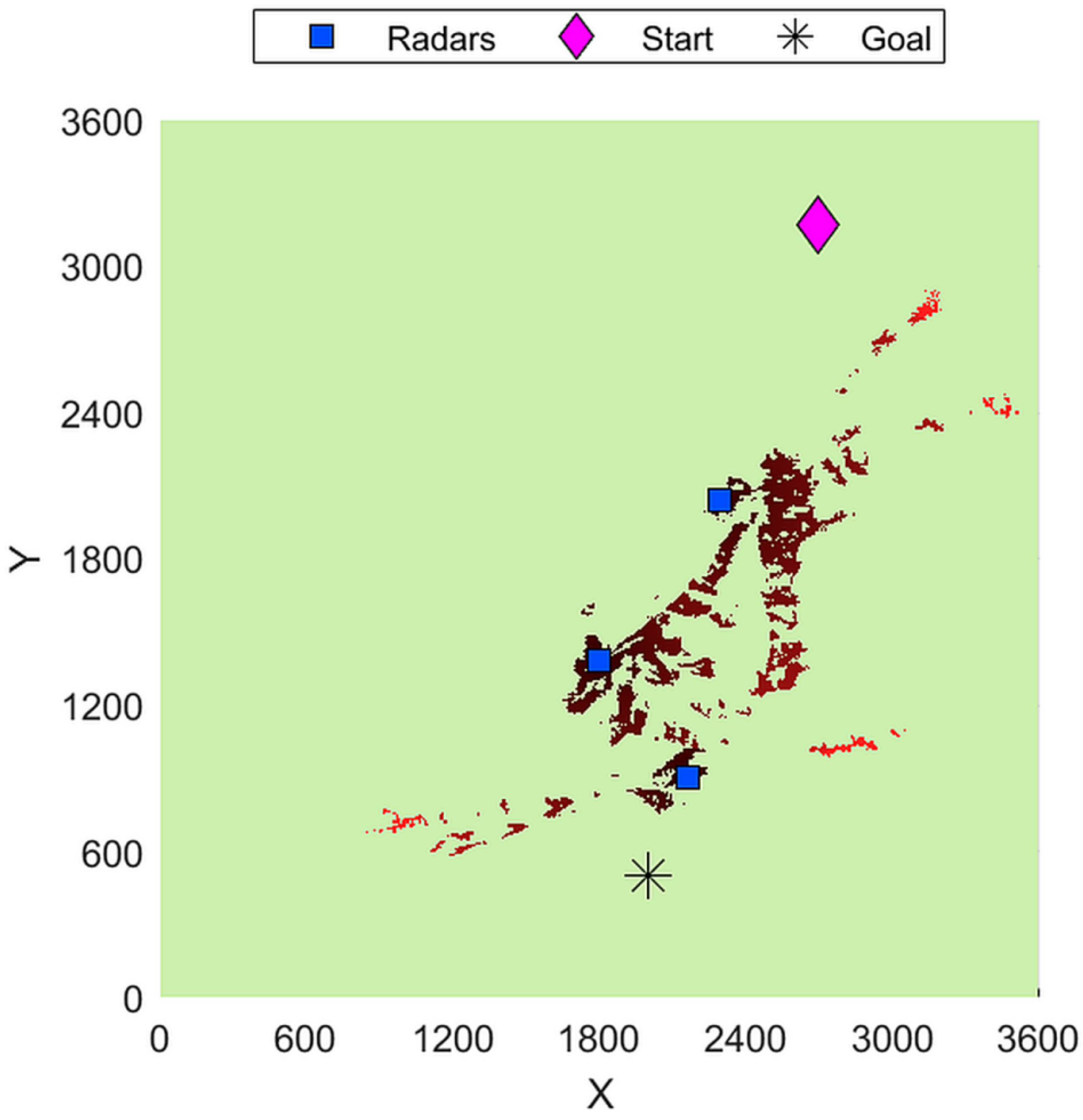
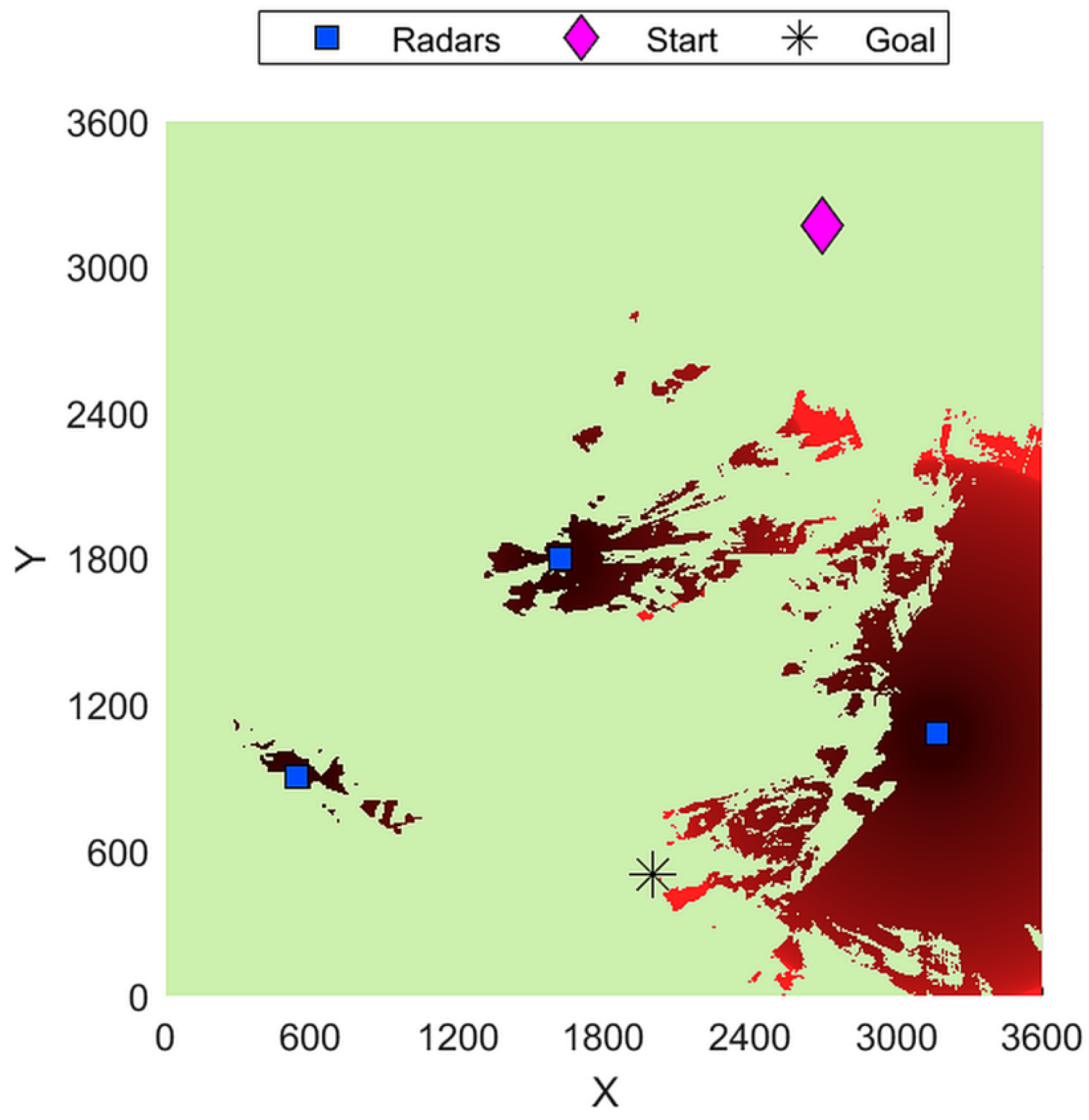
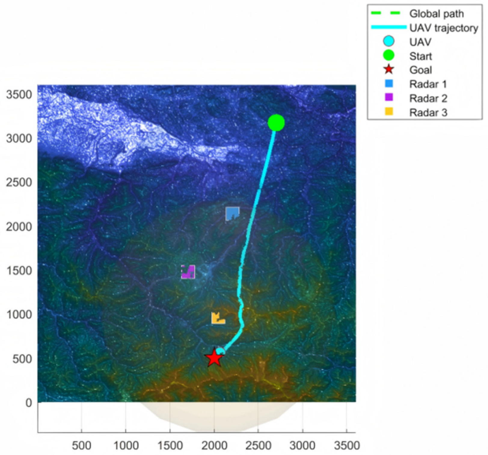
With the above parameter settings, terrain data ASTGTMV003_N39W106 [76] are loaded. The resulting global risk heat map is shown in Figure 10. Red regions indicate areas where the detectability metric exceeds the threshold η , whereas green regions indicate areas below η .
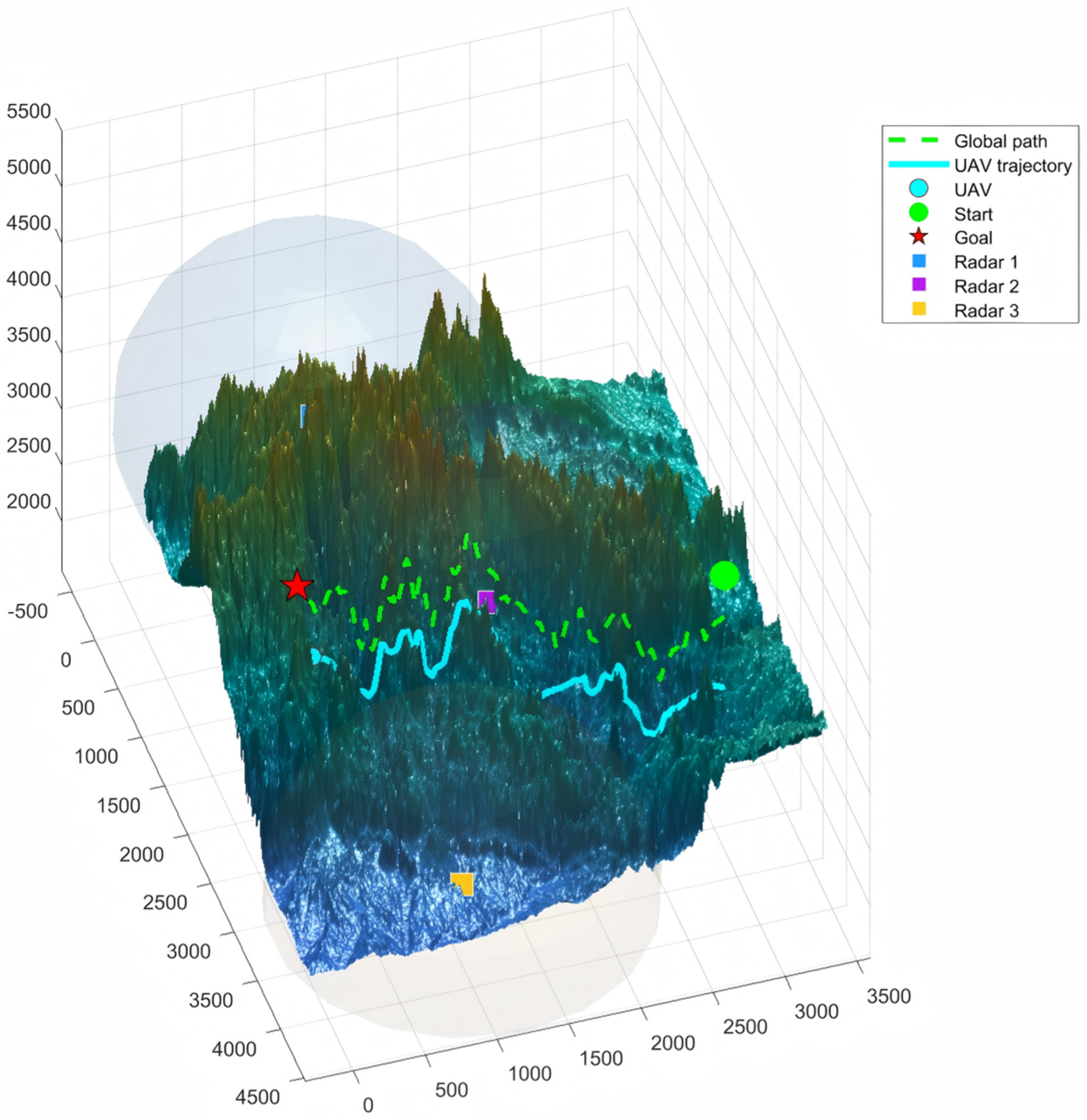
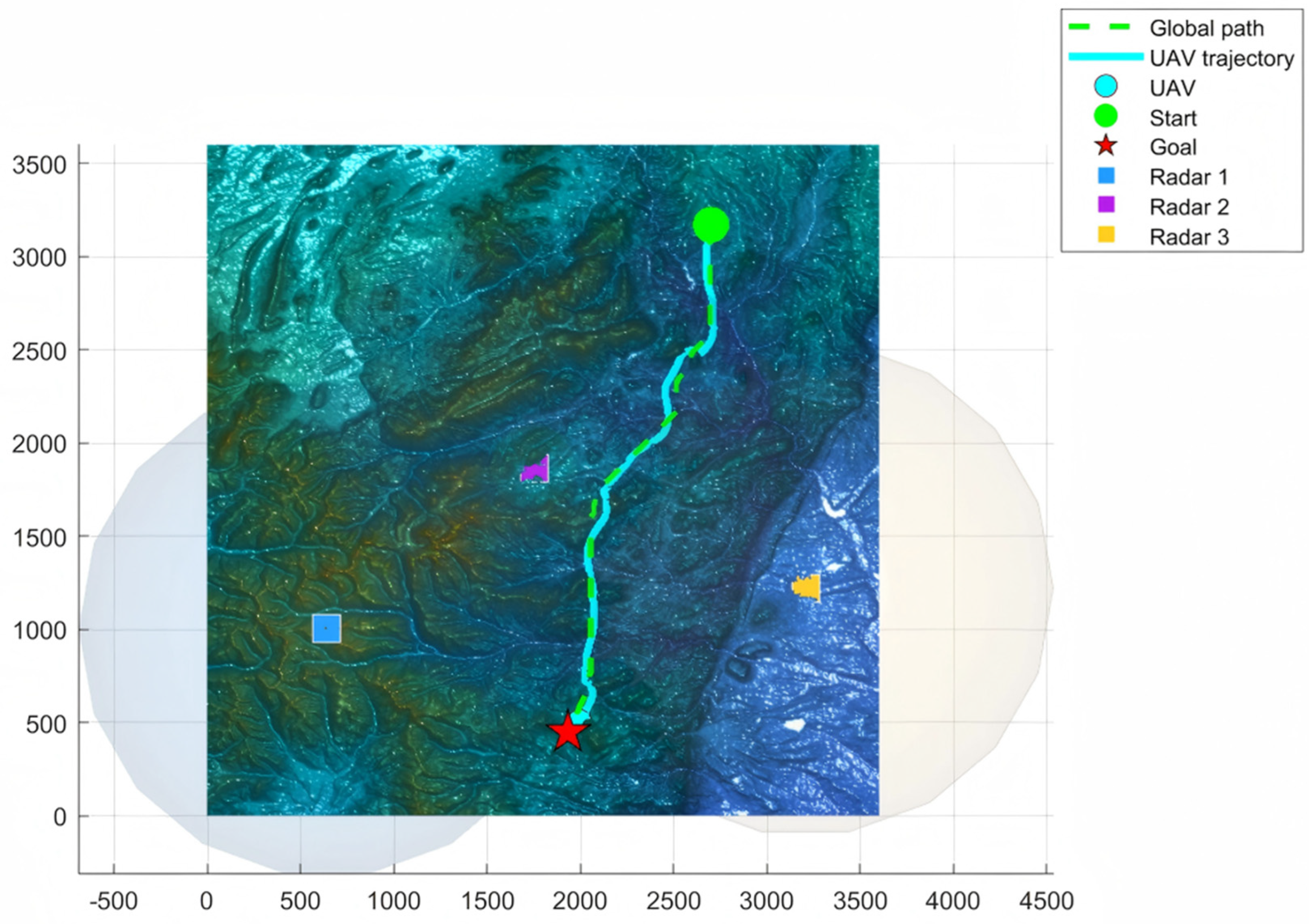
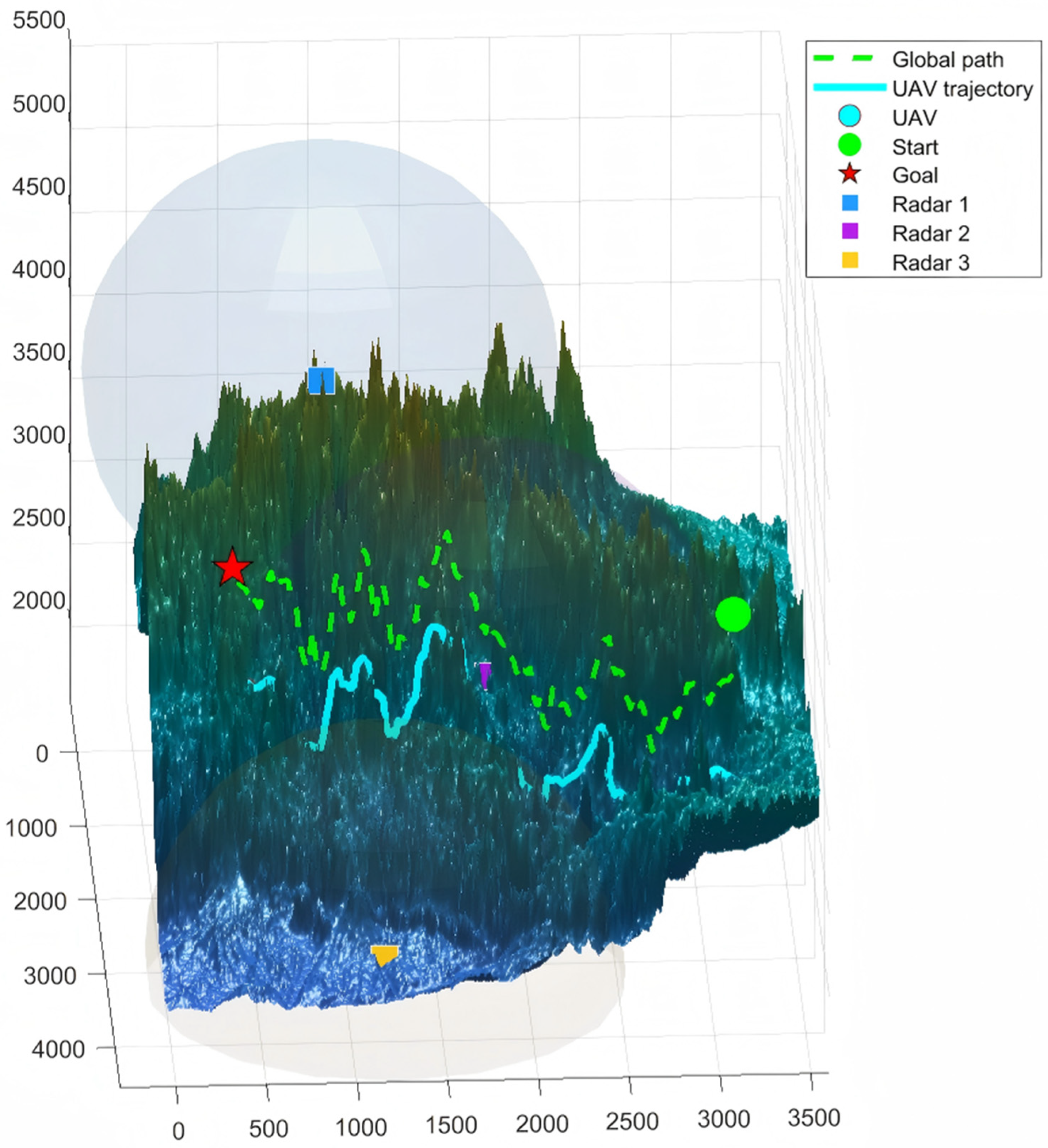
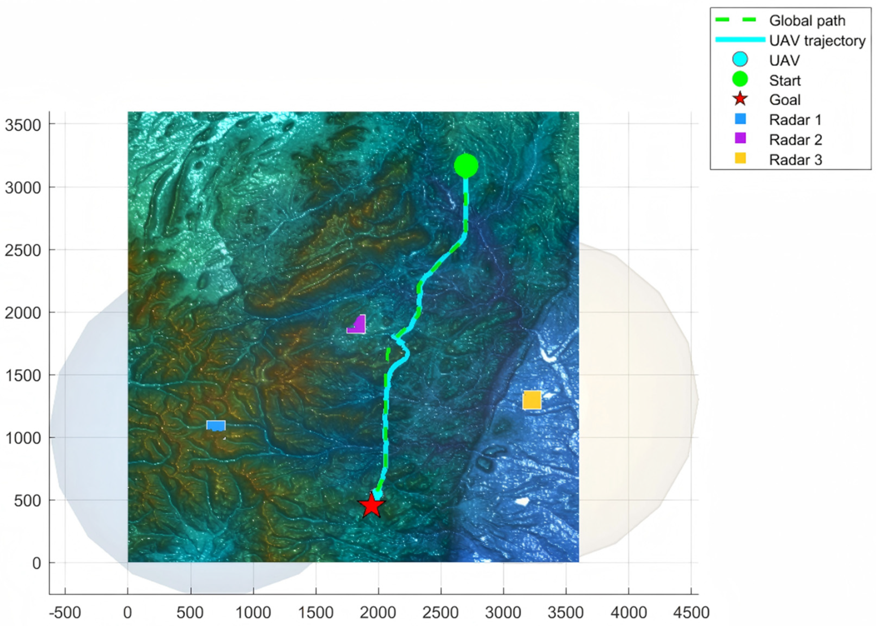
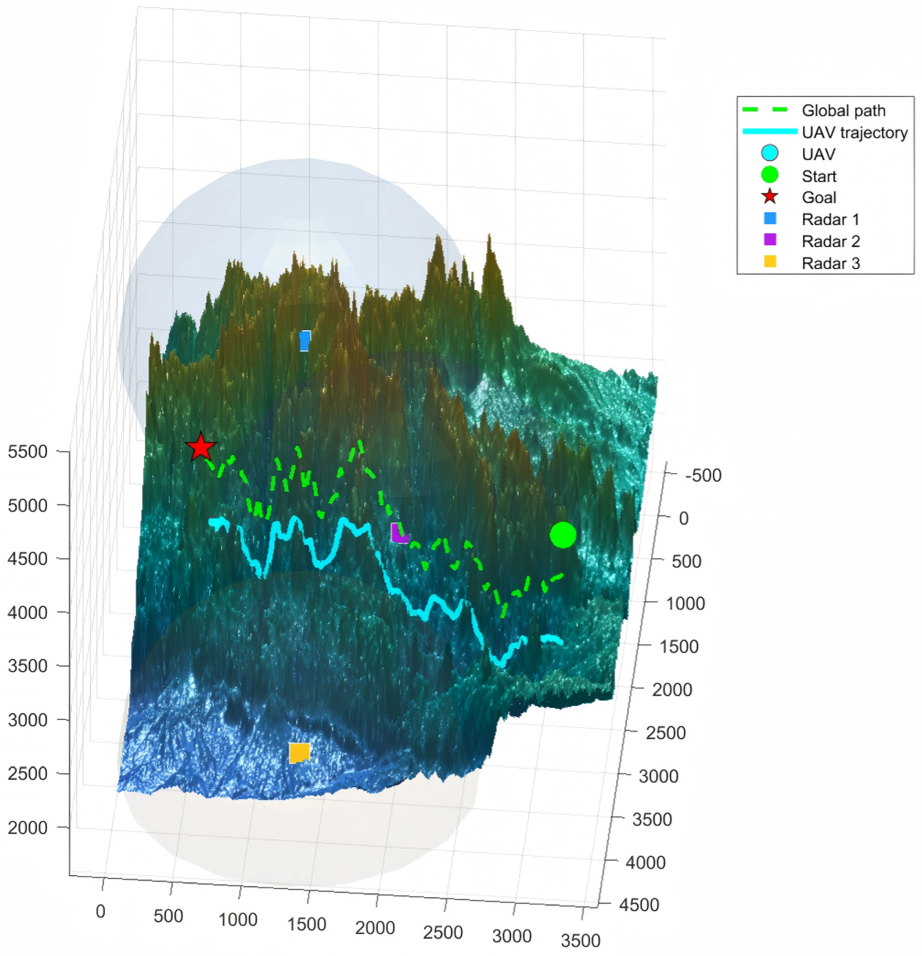
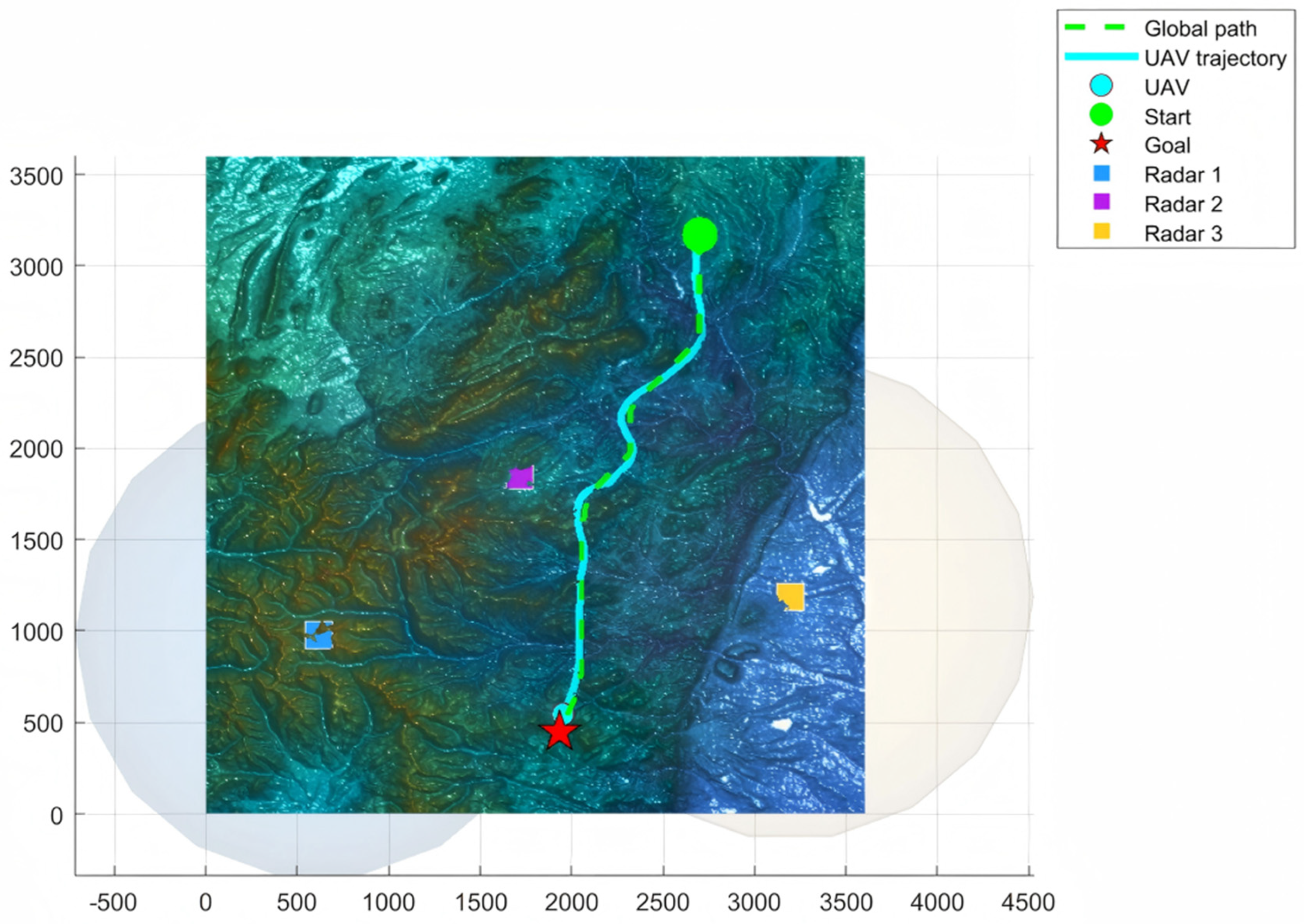
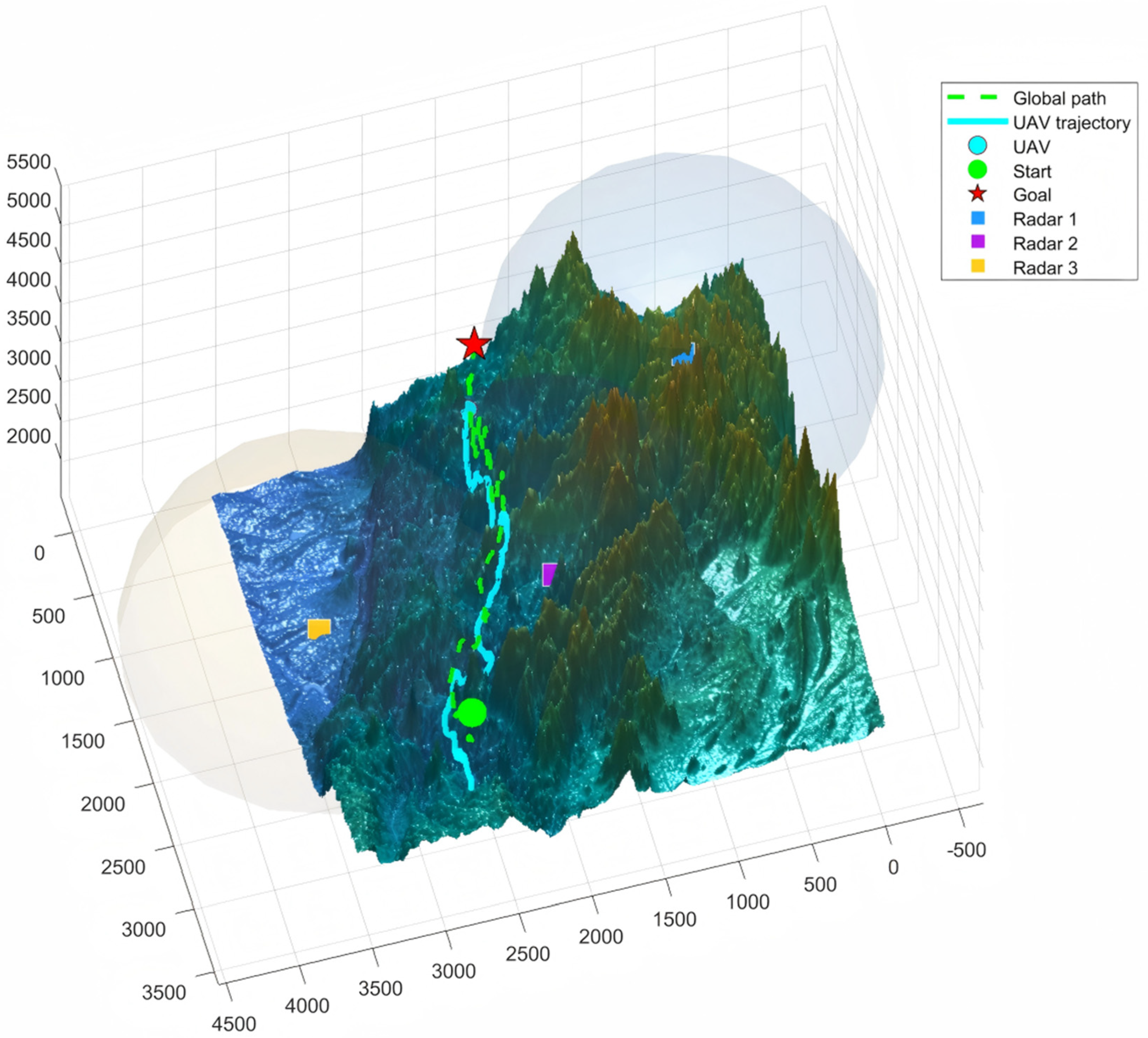
Figure 11 and Figure 12 present the two-dimensional and three-dimensional views, respectively. By comparing Figure 11 and Figure 10, it can be observed that the overall trajectory mainly follows the global route planned by Risk-A*, which guides the UAV to traverse the globally low-risk (green) region. In addition, when passing near Radar 2, the trajectory is adjusted online by the MPC algorithm to ensure that the UAV is not successfully detected by hostile radars throughout the flight.
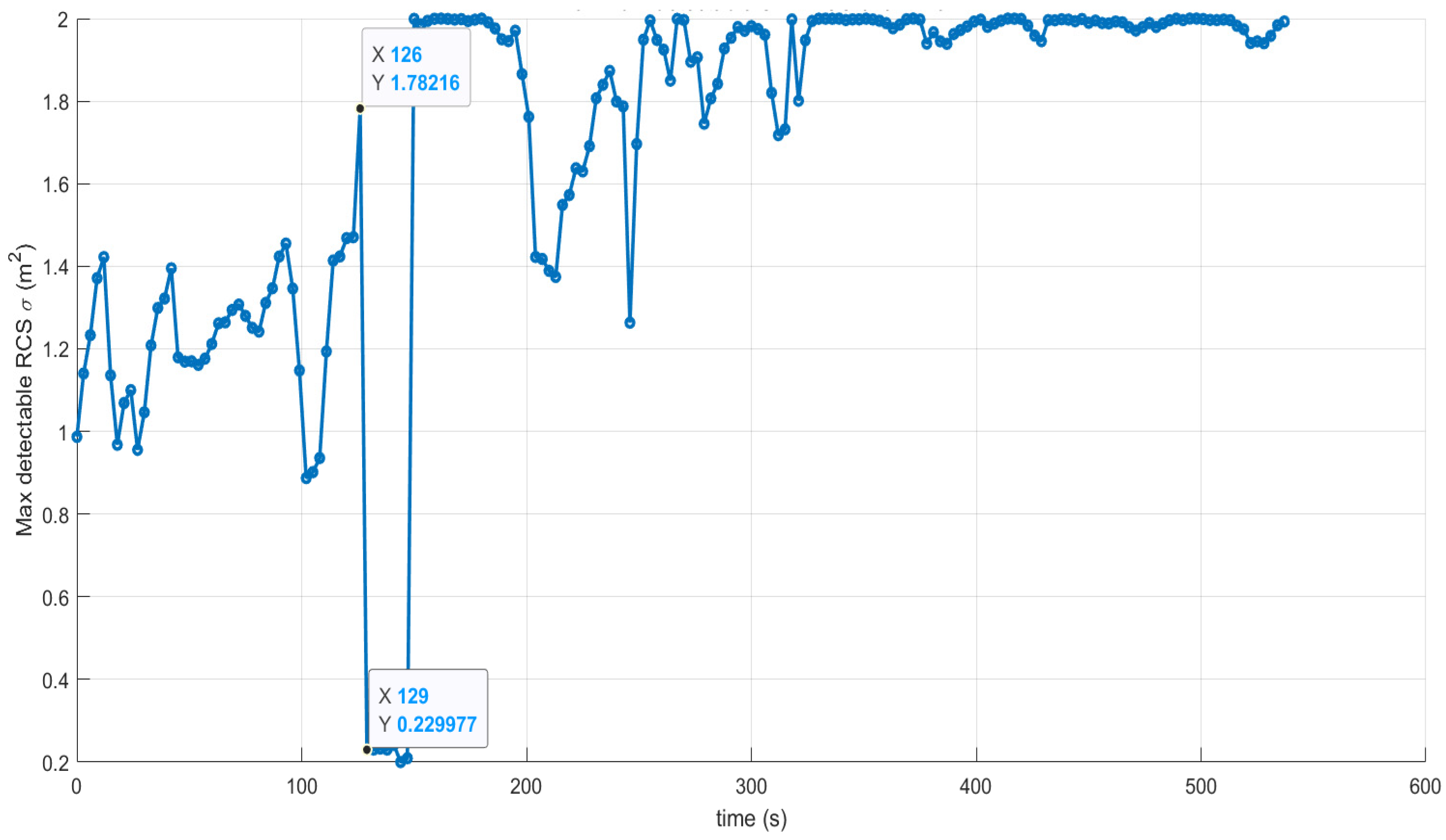
The LOS condition over the entire flight is analyzed, as shown in Figure 13. The global LOS equals 1 only during a short interval (129–156 s). As shown in Figure 14, the global effective detectability M ( ) never exceeds the prescribed threshold η = 7132 . Therefore, no exposure event occurs during the mission.
To evaluate the comprehensive performance of the proposed Risk-A*-MPC framework under complex mountainous terrain and dynamic radar-based sensing constraints, three representative global reference planners, namely Theta*, D* Lite, and RRT*, are selected as baselines and combined with the same local MPC executor. For all methods, the same terrain dataset, start-goal pair, radar-patrol configuration, UAV kinematic constraints, local MPC parameter settings, radar detection model, and detection threshold are used. The only planned difference is the global reference-path generation strategy. This setting ensures that the comparison reflects whether the global planner can provide a reference path with sufficient detection-risk margin for the common local MPC executor. The comparative results are reported in Table 1.

4.2.5. Scenario 2: Terrain Zone 2 with One Nominal Start-Goal Pair

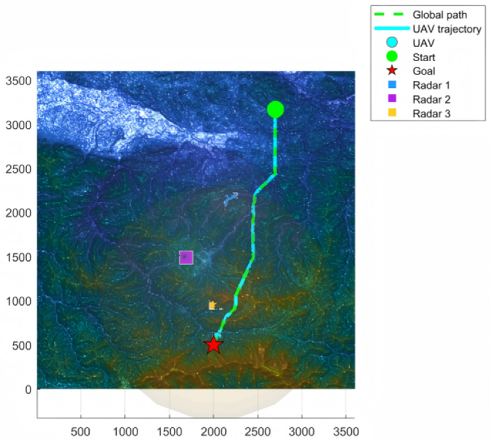
To examine whether the observed performance trend persists in a second mountainous-terrain setting, additional tests are conducted on Terrain Zone 2 generated from the ASTGTMV003_N33E107 dataset [68]. The corresponding global risk heat map is shown in Figure 15.
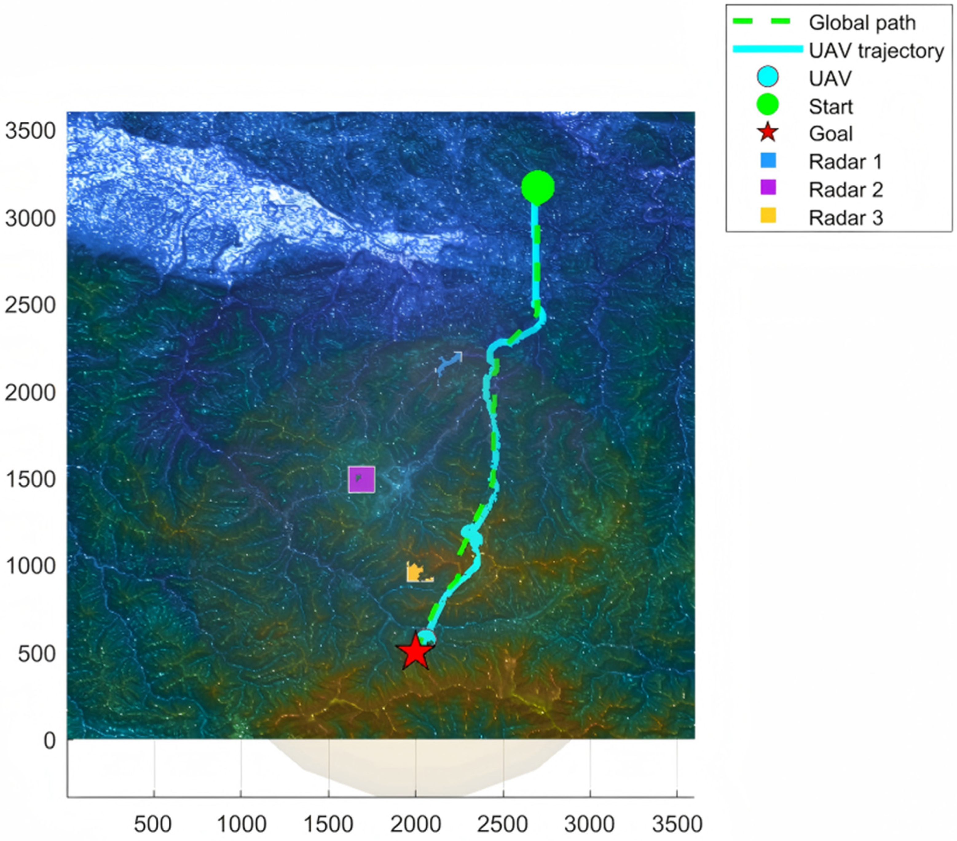
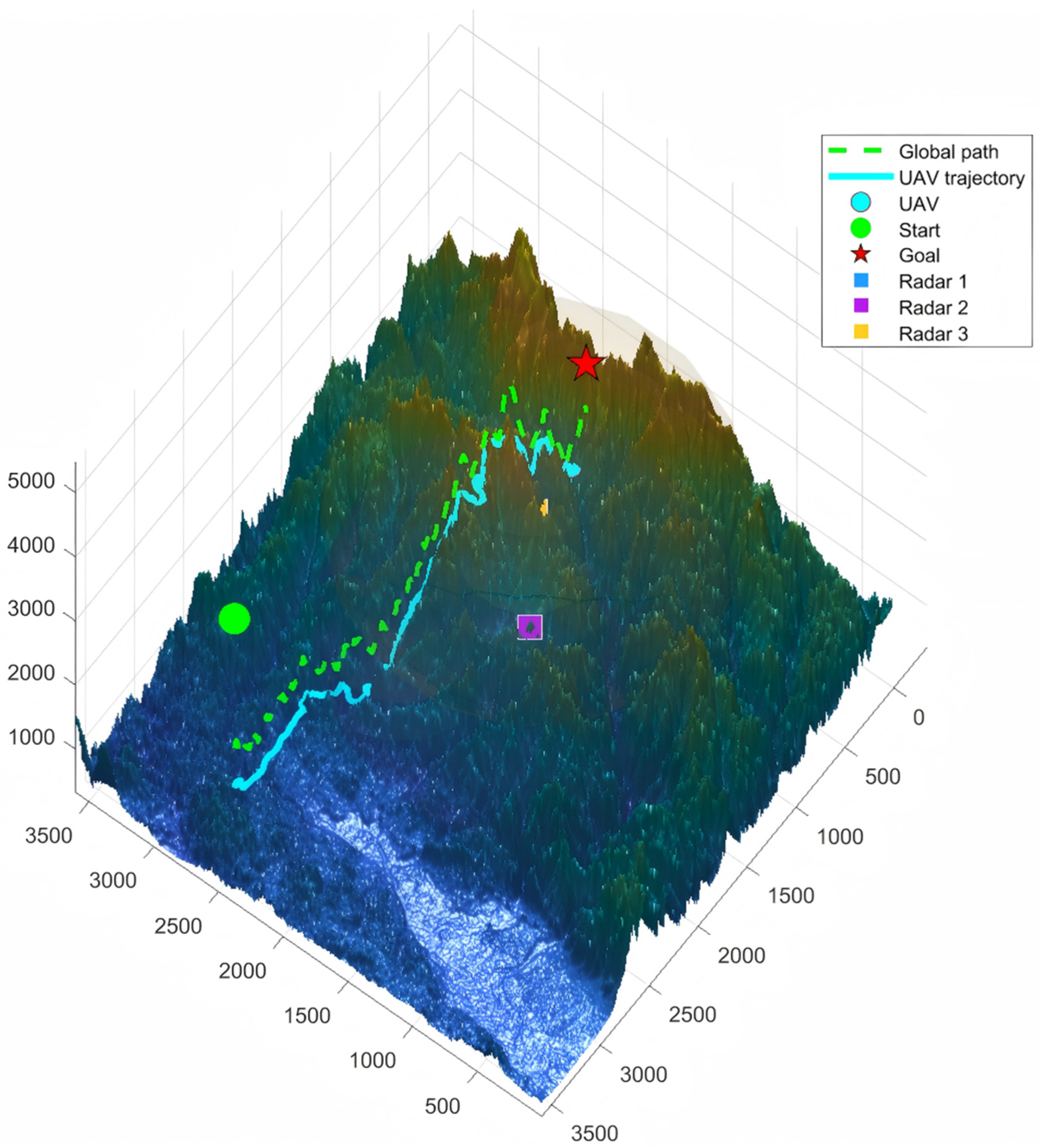
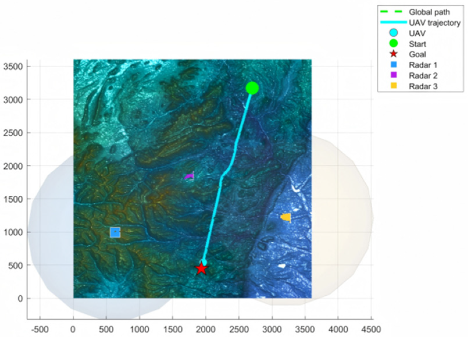
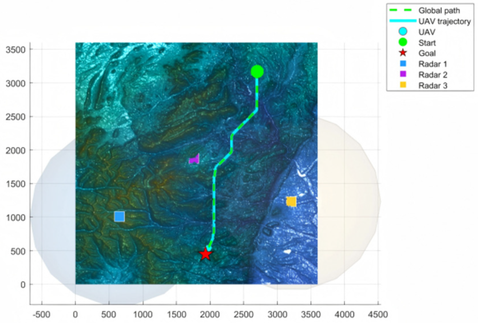
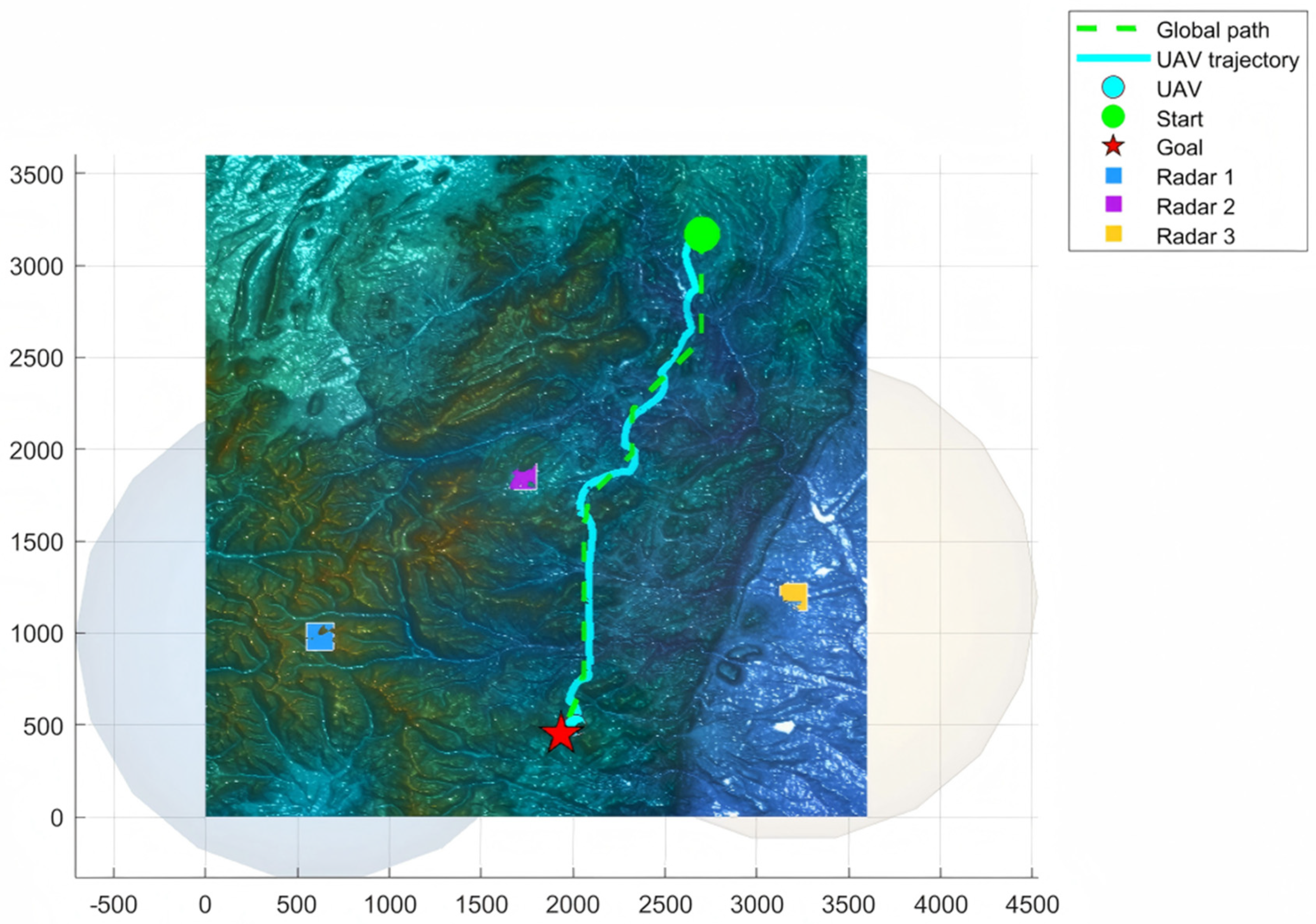
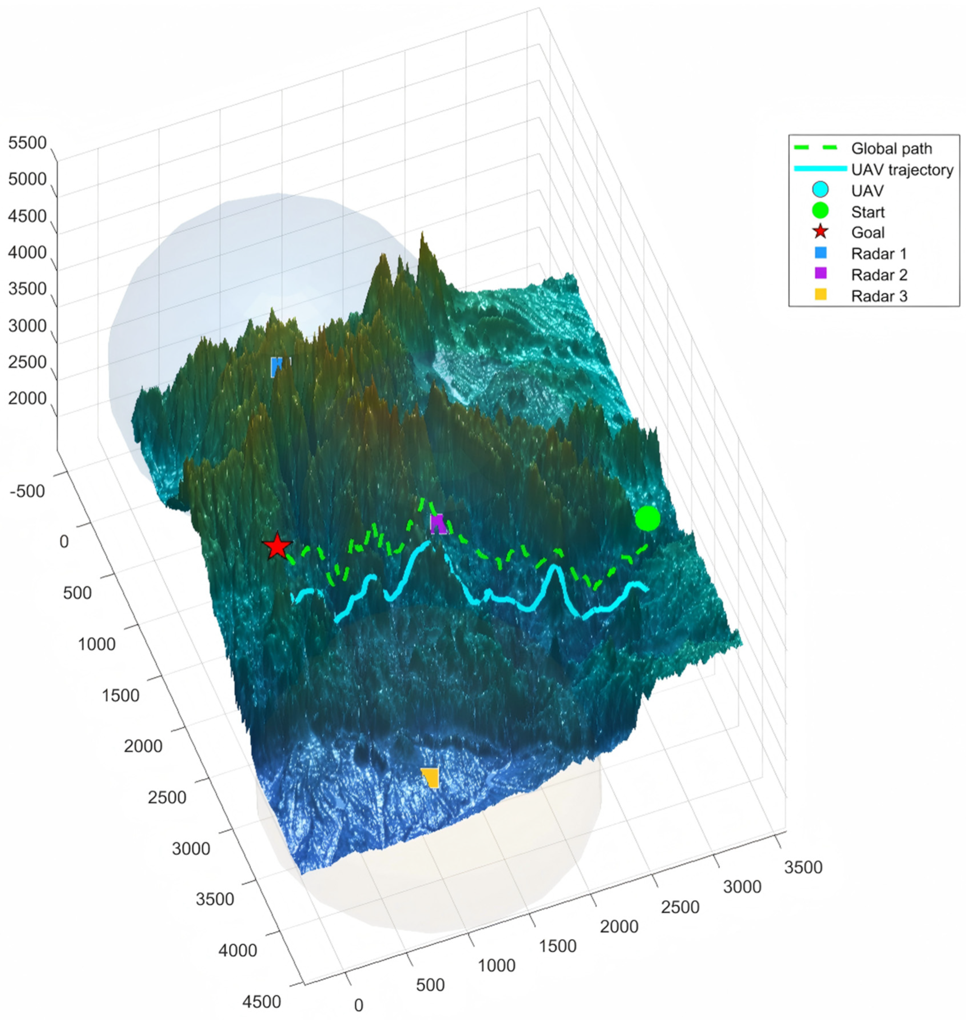
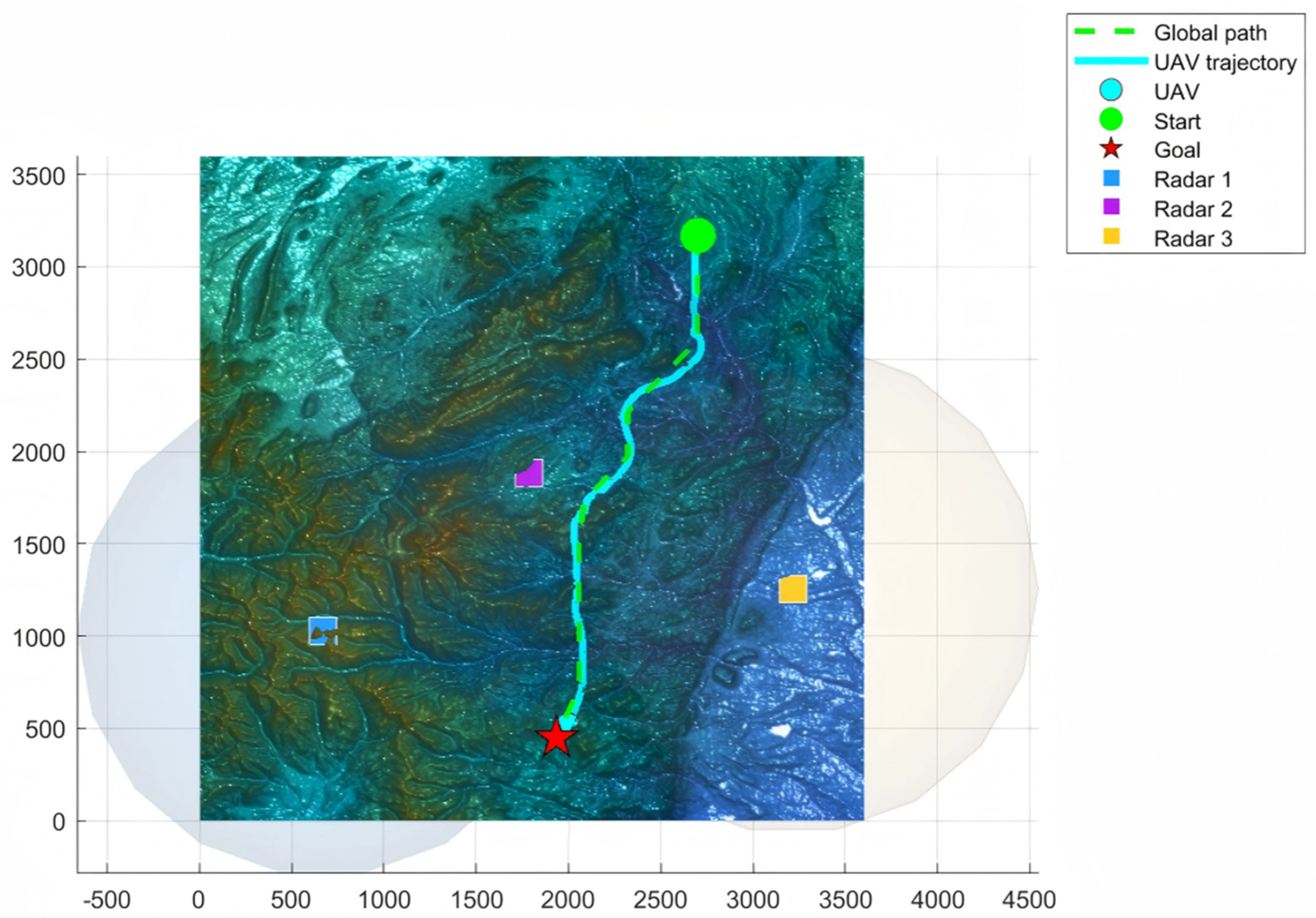
Figure 16 and Figure 17 present the two-dimensional and three-dimensional views, respectively. By comparing Figure 16 and Figure 15, it can be seen that the overall trajectory mainly follows the global route planned by Risk-A*, guiding the UAV through the globally low-risk (green) region. In addition, near Radar 3, online adjustments are performed by the MPC algorithm to account for radar motion, ensuring that the UAV is not successfully detected by hostile radars during the mission.
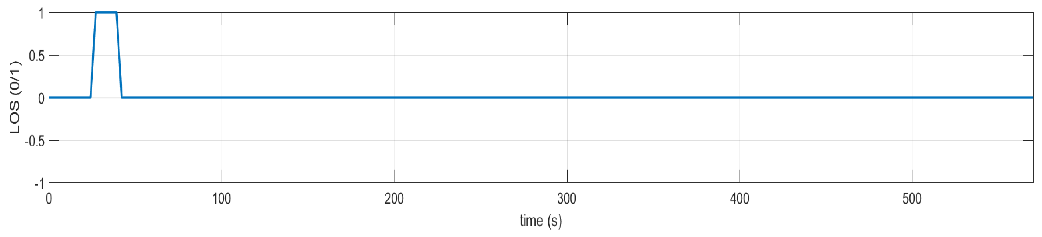
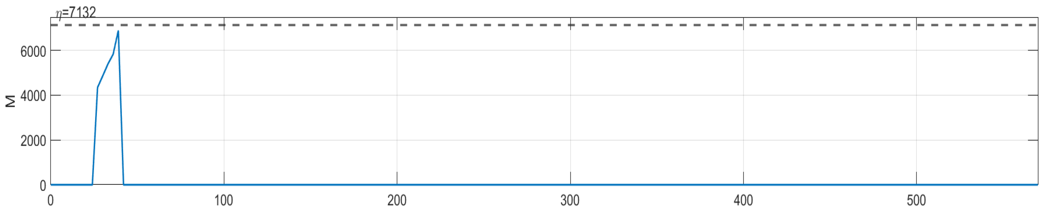
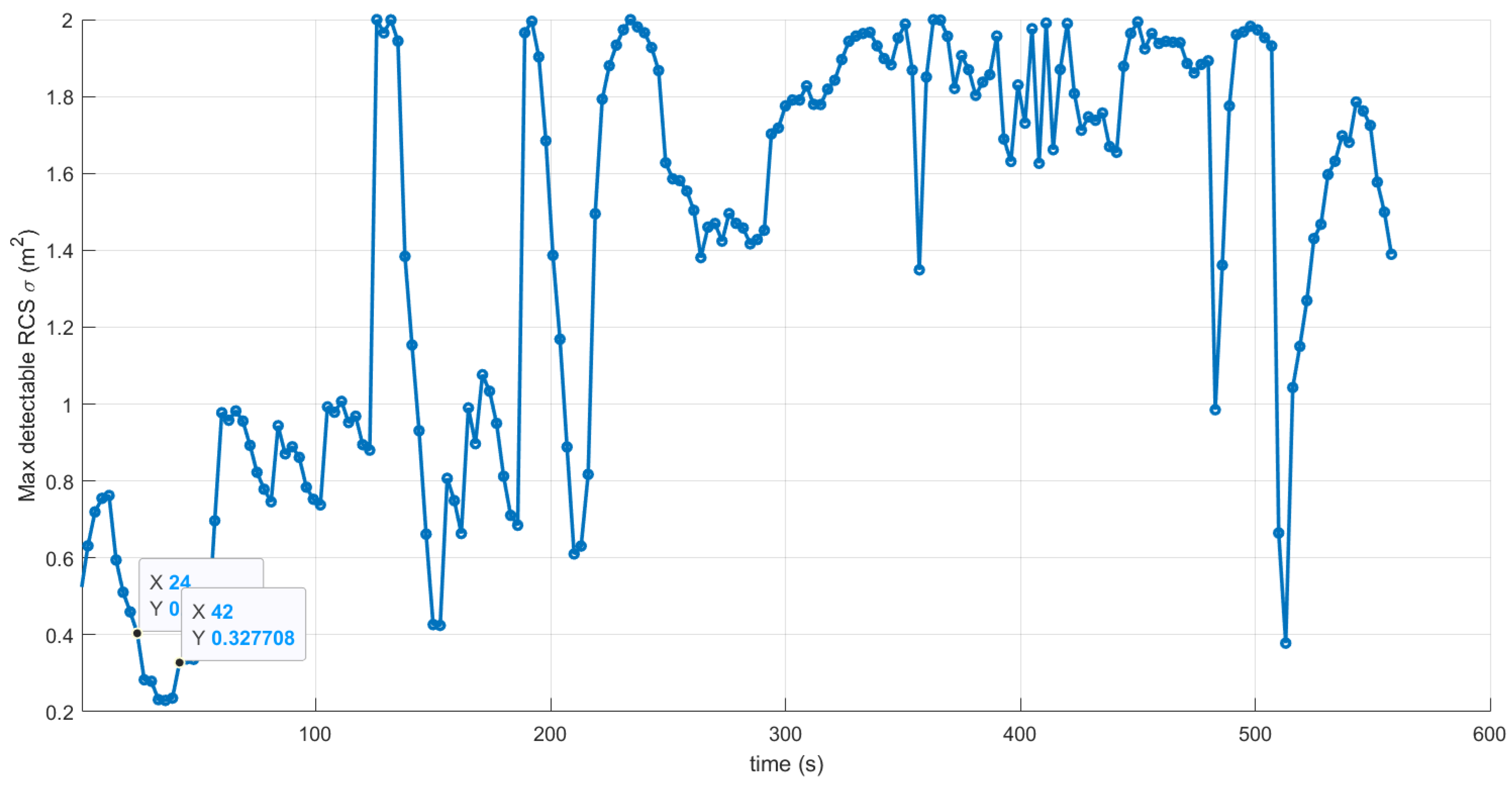
The results obtained by the Risk-A*-MPC framework in Scenario 2 are illustrated above. The LOS condition over the entire flight is analyzed. As shown in Figure 18, the global LOS equals 1 only during a short interval (24–42 s). As shown in Figure 19, the global effective detectability M ( ) never exceeds the prescribed threshold η = 7132 ; this indicates that the entire flight can be completed with zero exposure.
Under identical conditions, 50 independent trials are conducted, and the statistical results are summarized as follows.
Pairwise comparisons were conducted between Risk-A*-MPC and each baseline-MPC variant using two-sided Welch’s t-tests for T, L, and LOS-visible duration. SR, nexp, and exposed-trial Texp were reported descriptively and were not included in the Welch’s t-test analysis; p-values smaller than 0.001 are reported as p < 0.001.

4.2.6. Comparative Result Analysis

Table 1 and Table 2 present the descriptive comparison between the proposed method and three baseline-MPC variants under identical terrain conditions and the same radar detection model, where T, L, and LOS-visible duration are reported as mean ± SD with 95% CIs, whereas exposed-trial Texp is reported as mean ± SD only over exposed trials; Table 3 reports the pairwise Welch’s t-test results for T, L, and LOS-visible duration. Overall, the proposed Risk-A* + MPC framework achieves a more favorable balance between safety (success rate SR and exposure time Texp) and mission efficiency (total flight time T and path length L). In addition to the mean values, the standard deviations and 95% CIs reported in Table 1 and Table 2 further reveal the stability, uncertainty range, and consistency of the different methods across repeated independent trials.
(1)
Safety comparison
From the mission success rate SR and the exposed-trial statistics, it can be observed that the proposed Risk-A*-MPC framework consistently achieves SR = 1 under the prescribed detection threshold η , with n exp = 0 in both scenarios. The baseline-MPC variants are evaluated with the same local MPC executor, the same UAV kinematic constraints, the same radar detection model, and the same exposure-time evaluator. Their nonzero exposure times should therefore not be interpreted as being caused by different MPC constraints or different detection thresholds. Instead, they arise because Theta*, D* Lite, and RRT* generate geometry-oriented reference paths that do not explicitly construct a spatio-temporal detection-feasible corridor. Consequently, these reference paths may guide the UAV close to, or even into, regions where the detection-risk margin is too small. Under the finite prediction horizon, bounded turn/climb rates, and finite control-candidate set of the common MPC executor, the local planner may then have no detection-feasible rollout available. In such cases, the executed trajectory is counted as a safety failure when the same range-gating, LOS, and radar-equation threshold tests indicate threshold exceedance.
The descriptive results in Table 1 and Table 2 and the pairwise Welch’s t-test results in Table 3 support this interpretation. In both scenarios, the proposed Risk-A*-MPC framework descriptively attains the highest SR and yields n exp = 0 , indicating that no detection-threshold exceedance occurred in the 50 repeated executions. This indicates that the zero-exposure property is achieved consistently rather than occasionally. The pairwise Welch’s t-test results further quantify the differences in the all-trial continuous metrics, while exposure safety is compared descriptively using SR, nexp, and exposed-trial Texp. By comparison, the baseline-MPC variants produce exposed trials and nonzero exposed-trial Texp values, showing that detection-threshold exceedance still occurs in some repeated executions. In Scenario 1, Theta*-MPC, D* Lite-MPC, and RRT*-MPC yield Texp values of 20.3 ± 8.7 s, 14.6 ± 6.3 s, and 18.9 ± 9.5 s, respectively, while in Scenario 2 the corresponding values are 12.4 ± 5.8 s, 8.7 ± 4.1 s, and 11.5 ± 5.4 s. These results indicate that the main advantage of the proposed method lies in maintaining local MPC feasibility by providing a globally structured detection-risk-aware corridor, rather than merely relying on the same local MPC module to recover from an unfavorable global reference path.
(2)
Efficiency comparison
In terms of total flight time T and path length L, the proposed method incurs a moderate and controlled increase in mission time and path length to ensure safety. Compared with other methods, the global reference path generated by Risk-A* tends to exploit terrain masking to traverse low-risk regions. Although this strategy increases geometric path length and flight time in the tested scenarios, it significantly reduces exposure time. This demonstrates that the performance gain primarily stems from risk modeling and safe corridor selection, rather than simply detouring by excessively increasing path length.
The mean ± SD statistics provide additional insight into this trade-off. In Scenario 1, the proposed method yields T = 555.0 ± 11.2 s and L = 92,500 ± 1580 m, whereas in Scenario 2 it yields T = 588.6 ± 13.4 s and L = 98,102 ± 1740 m. These values are slightly larger than those of Theta*-MPC, D* Lite-MPC, and RRT*-MPC in terms of the mean, which is consistent with the original observation that the proposed framework may require somewhat longer flight time and path length in order to maintain a safer low-risk corridor. However, the standard deviations of T and L for the proposed method remain comparatively small in both scenarios. In particular, the variability of T and L is lower than that of Theta*-MPC and RRT*-MPC, and is also smaller than that of D* Lite-MPC. Therefore, the slightly increased mean flight time and path length should be interpreted as a controlled and repeatable safety-oriented trade-off, rather than as unstable planning behavior caused by occasional extreme detours.
(3)
Relationship between LOS duration and exposure
It is important to emphasize that LOS = 1 is a necessary condition for successful detection, but it does not inevitably lead to the detectability metric M ( ) exceeding the threshold η . Exposure is jointly determined by the range gating condition and the detectability threshold. Therefore, the occurrence of short intervals with LOS = 1 without exposure is not contradictory. The decisive factor is whether the effective detectability M ( ) exceeds η . Through the combination of a globally safe reference path and local dynamic refinement, the proposed method ensures that even when short-duration LOS = 1 events occur, the UAV can dynamically adjust its RCS to maintain M ( ) < η , thereby achieving a significant reduction in Texp.
The LOS-visible duration results in Table 1 and Table 2, together with the corresponding p-values in Table 3, further clarify this point. In Scenario 1, the proposed method has a LOS-visible duration of 26.9 ± 3.0 s [26.0, 27.8]. It is significantly lower than that of Theta*-MPC and RRT*-MPC (p = 0.023 and p = 0.002, respectively), while it is only numerically lower than that of D* Lite-MPC and the difference is not statistically significant (p = 0.077). In Scenario 2, the proposed method has a LOS-visible duration of 18.0 ± 4.3 s [16.8, 19.2], which is significantly lower than that of Theta*-MPC (p < 0.001), whereas the differences relative to D* Lite-MPC and RRT*-MPC are not statistically significant (p = 0.526 and p = 0.226, respectively). More importantly, despite the occurrence of LOS-visible intervals, the proposed framework yields nexp = 0 in both scenarios, indicating that no detection-threshold exceedance occurs in the 50 repeated executions. This confirms that LOS visibility alone does not determine exposure; instead, exposure is jointly determined by LOS visibility, range gating, detection-threshold exceedance, and heading-dependent RCS modulation.
Computational time was further evaluated to support the real-time execution claim for the online MPC layer. Runtime was measured as wall-clock time in MATLAB R2023b on a workstation equipped with an Intel Core i9-14900HX CPU and 64 GB RAM running Windows 11; no MATLAB parallel pool was used during the online MPC timing test. MPC solve time was recorded at every control cycle in the two main terrain-zone scenarios, and the reported statistics were computed over all MPC updates from the 50 repeated executions in each scenario. In Scenario 1, the mean MPC solve time was 0.286 ± 0.092 s, the 95th percentile was 0.472 s, and the maximum solve time was 0.684 s. In Scenario 2, the mean MPC solve time was 0.331 ± 0.108 s, the 95th percentile was 0.548 s, and the maximum solve time was 0.812 s. No deadline violation was observed among the recorded MPC updates in either main terrain-zone scenario, because every recorded solve time remained below the 3 s control update period. These results demonstrate that the online MPC layer satisfies the real-time execution requirement on the tested computational platform for the two main terrain-zone scenarios. The initial global Risk-A* planning and lower-frequency replanning are outside the 3 s local MPC update loop and are therefore considered separately from the online MPC real-time budget. In summary, although mainstream baselines exhibit advantages in geometric optimality and replanning efficiency, they are not specifically designed for the “hard detection constraint + dynamic radar detectability” scenario studied in this work. The proposed Risk-A*-MPC framework integrates a “global low-risk corridor” with “local hard-constrained correction,” achieving higher observed mission success rates, fewer exposed trials, lower exposed-trial exposure levels, and more stable performance across repeated trials while avoiding excessive online computational burden, thereby validating the overall superiority of the framework.


4.3. Ablation Study

To further evaluate the contribution of each module in the Risk-A* + MPC framework, ablation experiments are conducted by separately removing the global Risk-A* planner and the local MPC module. Each variant is executed 50 times under identical experimental conditions, and the same evaluation metrics are recorded. The corresponding results are summarized in Table 4 and illustrated in Figure 20 and Figure 21.
The results obtained on the terrain map in [68] are reported in Table 5 and Figure 22 and Figure 23.

4.4. Effect of Dynamic RCS Modulation

To validate the impact of dynamic RCS modulation on the effective detectability M ( ) , we analyze the time-varying RCS behavior observed in the experiments conducted on the terrain map in [76]. As illustrated in Figure 24, at t = 126   s the UAV becomes visible to the radar (i.e., LOS = 1 ), due to insufficient terrain masking along the flight path. At this moment, the UAV adjusts its heading-related RCS state at t = 126   s to reduce the modeled effective RCS, as shown in Figure 25. As shown in Figure 26, this adjustment effectively prevents the effective detectability M ( ) from exceeding the detection threshold η .
An analysis of the results obtained on the terrain map in [68] shows that, during the time interval of 24–42 s, no terrain masking is present along the flight path, resulting in LOS = 1 , as shown in Figure 27. During this interval, the UAV adjusts its heading-dependent RCS configuration to reduce the modeled effective RCS, as shown in Figure 28, thereby ensuring that the effective detectability M ( ) never exceeds the detection threshold η , as shown in Figure 29.

4.5. Parameter-Sensitivity and Robustness Analysis

To explicitly evaluate the parameter sensitivity and robustness of the proposed framework, the UAV flight speed and radar moving speed are varied while keeping the remaining experimental settings unchanged. These tests examine whether the proposed Risk-A*-MPC framework can maintain no detection-threshold exceedance under different dynamic conditions and radar-relative geometries.

4.5.1. Effect of UAV Flight Speed

(1) Keeping all other parameters unchanged, the UAV flight speed is reduced to 400 km/h. The resulting planned trajectories are shown in Figure 30 and Figure 31.
From the planned paths, it can be observed that the reduced UAV speed enlarges the effective detection region of the moving Radar 2. In response, the Risk-A* planner generates a global path that more closely follows terrain-masked regions. Meanwhile, the MPC controller further refines the trajectory locally to maintain safety. As shown in Figure 32 and Figure 33, the global LOS remains 0 throughout the entire flight, indicating that the UAV completely avoids radar visibility.
The algorithm is executed 50 times, and the summary statistics are reported in Table 6.
(2) Keeping all other parameter settings unchanged, the UAV flight speed is increased to 800 km/h. The planned trajectories are shown in Figure 34 and Figure 35.
As shown in Figure 36, although there exist time intervals during flight when the radar has line-of-sight visibility (i.e., LOS = 1 ), the planned trajectory never causes the global effective detectability M ( ) to exceed the threshold η , as illustrated in Figure 37. Therefore, the mission is completed with zero exposure.
The algorithm is executed 50 times, and the summary statistics are reported in Table 7.

4.5.2. Effect of Radar Moving Speed

(1)
Radar speed: 6 m/s
As shown in Figure 38 and Figure 39, the planned trajectory under the radar speed of 6 m/s is similar to that obtained when the radar speed is 8 m/s. As shown in Figure 40 and Figure 41, the global LOS remains 0 throughout the entire flight, indicating that the UAV faces no risk of being detected.
The algorithm is executed 50 times, and the summary statistics are reported in Table 8.
(2)
Radar speed: 10 m/s
The planned trajectories are shown in Figure 42 and Figure 43. With the increased radar moving speed, the UAV faces a higher potential exposure risk. As shown in Figure 44, the UAV experiences LOS = 1 for a total duration of 14 s. However, through dynamic RCS modulation, the effective detectability M ( ) never exceeds the prescribed threshold η . The corresponding effective-detectability profile is shown in Figure 45.
The algorithm is executed 50 times, and the summary statistics are reported in Table 9.
Through the above four groups of parameter-sensitivity experiments, the robustness of the proposed Risk-A*-MPC framework is further validated. By varying the UAV flight speed and radar moving speed, the proposed method is shown to effectively adapt to changes in flight duration, radar-relative geometry, LOS visibility, and heading-dependent RCS conditions. In all tested parameter settings, the proposed framework maintains SR = 1.00 with nexp = 0, indicating that no detection-threshold exceedance occurs under the evaluated parameter perturbations.

5. Discussion

This study addresses the low-altitude penetration path planning problem for fixed-wing UAVs operating in complex mountainous terrain under moving radar threats. We propose a dual-layer planning framework in which a global Risk-A* planner constructs a safety-margined low-risk corridor, while a local receding-horizon MPC refines the trajectory online under kinematic and stealth constraints. Terrain masking (LOS), range gating, and radar-equation-based thresholding are jointly incorporated into a unified hard-feasibility formulation, and an anisotropic heading-dependent RCS model is further introduced to capture the planning-level interaction among heading, detectability, and control. Across two representative terrain scenarios, ablation experiments, dynamic-RCS analyses, and robustness evaluations under varying UAV and radar speeds, the proposed framework consistently maintains the effective detectability below the prescribed threshold within the adopted simplified deterministic simulation setting, while revealing a clear safety-oriented trade-off among exposure time, path length, and total flight time. In the two main comparative scenarios, Risk-A*-MPC achieves SR = 1.00 with nexp = 0, whereas the baseline-MPC variants produce exposed trials with nonzero exposed-trial Texp values. This safety gain is obtained at the cost of moderately increased path length and total flight time: compared with the shortest baseline in each scenario, path length and total flight time increase from 84,369 m and 506.2 s to 92,500 m and 555.0 s in Scenario 1, and from 87,235 m and 523.4 s to 98,102 m and 588.6 s in Scenario 2. Because the horizontal ground-relative speed is fixed in the adopted planning model, the increases in path length and total flight time are approximately proportional rather than independent penalties. Therefore, the proposed framework does not simply pursue a longer detour; instead, it deliberately exchanges a bounded and repeatable efficiency cost for zero detection-threshold exceedance under the tested deterministic conditions. The real-time executability of the online MPC layer was quantitatively evaluated by recording the MPC solve time at every control cycle in the two main terrain-zone scenarios. The maximum solve time was 0.684 s in Scenario 1 and 0.812 s in Scenario 2, corresponding to 22.8% and 27.1% of the 3 s control update period, respectively. Therefore, the local receding-horizon optimization was completed before the next control update for every recorded MPC update in these two main terrain-zone scenarios. The real-time claim in this study refers specifically to the online MPC layer. The global Risk-A* planner is executed before flight or at lower-frequency intelligence-update instants and is therefore not included in the 3 s local MPC update budget. In addition, Table 1, Table 2, Table 4, Table 5, Table 6, Table 7, Table 8 and Table 9 report (T), (L), and LOS-visible duration as mean ± standard deviation with 95% confidence intervals over all 50 trials, while exposed-trial Texp is reported as mean ± standard deviation over exposed trials together with nexp; together with the pairwise significance-test results for T, L, and LOS-visible duration in Table 3, these results indicate that the superiority of the proposed method lies not only in its average safety performance, but also in its repeatability, stability, and robustness across different experimental settings. The key advantage of the proposed framework lies in the complementarity between global conservative feasible guidance and local high-frequency executable correction:
(1) The Risk-A* global planner does not merely optimize geometric distance. Instead, it introduces a continuous risk cost on top of a hard “deterministic no-detection” baseline, producing a reference corridor with greater separation from the hard baseline.
(2) The local MPC performs receding-horizon optimization within a short prediction window. Hard constraints ensure that the predicted trajectory remains within the feasible region of the adopted planning model, while physically meaningful planning-level control variables, including heading rate and climb/descent rate, are optimized to generate smooth trajectories that are feasible under the reduced-order UAV kinematic constraints used in this study. This feasibility should not be interpreted as full six-degree-of-freedom flight-dynamic feasibility, because roll, pitch, actuator dynamics, and inner-loop tracking errors are not explicitly represented. Nevertheless, the above findings should be interpreted within the simplified simulation assumptions adopted in this study. In particular, the radar-detection model is deterministic and threshold-based, and it does not explicitly model stochastic detection probability, clutter, multipath propagation, electronic countermeasures, or measurement uncertainty. A further limitation of the present framework is that the UAV is modeled using a reduced-order kinematic representation in which horizontal motion is described in a planar form and vertical motion is updated separately through terrain-coupled altitude variables, rather than through explicit full three-dimensional attitude dynamics. As a result, roll- and pitch-induced effects on vehicle motion and radar detectability are not directly represented.
Therefore, the conclusions of this study should be interpreted as being applicable primarily at the path-planning and guidance level, rather than as a full high-fidelity description of real-world UAV attitude dynamics. In addition, the RCS model only depends on the horizontal aspect angle; RCS variations induced by roll, pitch, elevation angle, frequency dependence, and detailed airframe scattering are not explicitly represented. Another limitation of this study is the limited diversity of the simulated mission cases. The evaluation is conducted on two DEM-based mountainous terrain zones, with one nominal start-goal pair and one radar-patrol configuration specified in each terrain zone. The 50 repeated executions in each scenario are used to assess repeatability and variability under the same mission geometry, and should not be interpreted as 50 different terrain zones or 50 distinct start-goal pairs. Therefore, although the results demonstrate the feasibility and stability of the proposed framework under the tested conditions, its generalizability to a broader range of terrain zones, start-goal pairs, radar deployments, and mission geometries remains to be further validated. Future work will expand the evaluation to more terrain zones and more diverse start-goal pairs.

6. Conclusions

This paper focuses on low-altitude penetration missions in mountainous terrain under moving radar threats and proposes a dual-layer path planning framework subject to hard detection constraints. The global layer constructs a safety-margined reference path on a spatio-temporal risk map using Risk-A*, while the local layer employs a hard-constrained receding-horizon MPC to refine the trajectory online under kinematic and altitude constraints. By incorporating a heading-dependent anisotropic RCS model, the proposed method reduces the modeled radar detectability in scenarios where LOS becomes temporarily available.
This framework differs from previous radar-aware path-planning, MPC-based, and risk-based planning methods in that it does not rely on a single radar-risk cost, a standalone local radar-constraint MPC, or a generic risk field. Instead, it explicitly separates hard feasibility from soft risk optimization. The global layer first constructs a conservative no-detection-threshold-exceedance corridor, while the local layer refines the trajectory online using heading-dependent RCS modulation under the same detection-threshold constraint. This separation explains why the proposed method may produce slightly longer trajectories but achieves zero exposure more consistently than geometry-oriented baseline planners executed by the same MPC module.
Simulation experiments are conducted in representative DEM-based mountainous environments with dynamic radar patrol routes, and comparisons are made against baseline methods such as Theta*, D* Lite, and RRT*. The results show that, within the two tested DEM-based scenarios and under the adopted simplified deterministic simulation assumptions, the proposed method enables the UAV to complete the mission with zero exposure; this improvement in safety is achieved by accepting moderately longer total flight time and path length, which represents a deliberate safety-oriented trade-off rather than an unbounded loss of flight efficiency. Ablation studies further confirm the complementary roles of the global Risk-A* corridor and local MPC refinement in improving mission success, while the dynamic-RCS analysis illustrates how heading-dependent RCS modulation helps maintain the effective detectability below the detection threshold during LOS-visible intervals. Robustness evaluations suggest that the proposed algorithm retains stable zero-exposure performance under the tested variations in UAV speed and radar moving speed, although broader generalization requires validation under more diverse terrain, radar, and vehicle-model conditions. Runtime evaluation further confirms that, on the tested computational platform, every recorded online MPC update in the two main terrain-zone scenarios was completed within the prescribed 3 s control update period, with a maximum solve time of 0.812 s. Future work will focus on probabilistic and higher-fidelity radar-detection modeling, more refined treatment of detection uncertainty, coupling with natural environment factors such as wind fields, and incorporating explicit full three-dimensional attitude dynamics and more complete RCS representations beyond the horizontal-aspect-angle model to further improve physical fidelity, applicability, and engineering reliability in realistic operational settings. In addition, future studies will conduct hardware-in-the-loop validation and physical UAV flight experiments in representative mountainous environments to further evaluate the proposed framework using real flight trajectories, onboard navigation data, and radar-detection-related measurements when suitable UAV platforms, test sites, and sensing facilities become available.

Author Contributions

Conceptualization, Y.Q. and T.Y.; methodology, Y.Q. and T.Y.; software, Y.Q.; validation, Y.Q.; formal analysis, Y.Q.; investigation, Y.Q. and T.Y.; resources, Y.Q. and T.Y.; data curation, Y.Q.; writing—original draft preparation, Y.Q.; writing—review and editing, Y.Q.; visualization, Y.Q.; supervision, T.Y.; project administration, Y.Q., T.Y. and Y.L.; funding acquisition, Y.L. All authors have read and agreed to the published version of the manuscript.

Funding

This research received no external funding.

Data Availability Statement

The DEM data used in this study are publicly available from the Geospatial Data Cloud site, Computer Network Information Center, Chinese Academy of Sciences, under the dataset GDEMV3 30 M Digital Elevation Data. The dataset is available at: https://www.gscloud.cn/sources/accessdata/aeab8000652a45b38afbb7ff023ddabb?pid=302 (accessed on 6 March 2026). These data were derived from the publicly available ASTER GDEM V3 30 m digital elevation dataset, which was used to generate the DEM-based terrain for the simulations in this study.

DURC Statement

Current research is limited to autonomous aerial robotics and risk-aware low-altitude UAV path planning in complex mountainous environments, which is beneficial for terrain-aware navigation, emergency response, disaster monitoring, infrastructure inspection, and airspace safety assessment, and does not pose a threat to public health or national security. Authors acknowledge the dual-use potential of the research involving UAV path planning under radar-based sensing and detectability constraints and confirm that all necessary precautions have been taken to prevent potential misuse. The study is based on numerical simulations, public terrain data, and generic detection models, and does not provide operational deployment procedures, targeting strategies, or sensitive real-world system parameters. As an ethical responsibility, authors strictly adhere to relevant national and international laws about DURC. Authors advocate for responsible deployment, ethical considerations, regulatory compliance, and transparent reporting to mitigate misuse risks and foster beneficial outcomes.

Conflicts of Interest

The authors declare no conflicts of interest.

References

  1. Aggarwal, S.; Kumar, N. Path planning techniques for unmanned aerial vehicles: A review, solutions, and challenges. Comput. Commun. 2020, 149, 270–299. [Google Scholar] [CrossRef]
  2. Mozaffari, M.; Saad, W.; Bennis, M.; Debbah, M. A tutorial on UAVs for wireless networks: Applications, challenges, and open problems. IEEE Commun. Surv. Tutor. 2019, 21, 2334–2360. [Google Scholar] [CrossRef]
  3. Tang, C.; Abbatematteo, B.; Hu, J.; Chandra, R.; Martín-Martín, R.; Stone, P. Deep Reinforcement Learning for Robotics: A Survey of Real-World Successes. Annu. Rev. Control Robot. Auton. Syst. 2025, 8, 153–188. [Google Scholar] [CrossRef]
  4. Foehn, P.; Romero, A.; Scaramuzza, D. Time-optimal planning for quadrotor waypoint flight. Sci. Robot. 2021, 6, eabh1221. [Google Scholar] [CrossRef] [PubMed]
  5. Chan, Y.Y.; Ng, K.K.H.; Lee, C.K.M.; Hsu, L.T.; Keung, K.L. Wind dynamic and energy-efficiency path planning for unmanned aerial vehicles in the lower-level airspace and urban air mobility context. Sustain. Energy Technol. Assess. 2023, 57, 103202. [Google Scholar] [CrossRef]
  6. Chen, P.; Jiang, Y.; Dang, Y.; Yu, T.; Liang, R. Real-time efficient trajectory planning for quadrotor based on hard constraints. J. Intell. Robot. Syst. 2022, 105, 52. [Google Scholar] [CrossRef]
  7. Li, J.; Xiong, Y.; She, J.; Yu, A. Optimal path planning for unmanned aerial vehicles with multiple round-trip flights in coverage tasks. Robot. Auton. Syst. 2025, 189, 104970. [Google Scholar] [CrossRef]
  8. Wang, Y.; Wang, G. An adaptive and efficient path planning algorithm for UAV navigation in complex environments. Comput. Oper. Res. 2026, 185, 107296. [Google Scholar] [CrossRef]
  9. Zhao, Z.; Niu, Y.; Ma, Z.; Ji, X. A fast stealth trajectory planning algorithm for stealth UAV to fly in multi-radar network. In Proceedings of the 2016 IEEE International Conference on Real-time Computing and Robotics (RCAR), Angkor Wat, Cambodia, 6–9 June 2016. [Google Scholar] [CrossRef]
  10. Zhang, Z.; Wu, J.; Dai, J.; He, C. A novel real-time penetration path planning algorithm for stealth UAV in 3D complex dynamic environment. IEEE Access 2020, 8, 122758–122771. [Google Scholar] [CrossRef]
  11. Atayev, A.; Fliege, J.; Zemkoho, A. Trajectory optimization of unmanned aerial vehicles in the electromagnetic environment. Optim. Eng. 2025, 26, 159–198. [Google Scholar] [CrossRef]
  12. Su, M.; Chai, H.; Zhao, C.; Lyu, Y.; Hu, J. Lightweight obstacle avoidance for fixed-wing UAVs using entropy-aware PPO. Drones 2025, 9, 598. [Google Scholar] [CrossRef]
  13. Bassolillo, S.R.; Raspaolo, G.; Blasi, L.; D’Amato, E.; Notaro, I. Path planning for fixed-wing unmanned aerial vehicles: An integrated approach with Theta* and clothoids. Drones 2024, 8, 62. [Google Scholar] [CrossRef]
  14. Yu, S.; Park, J. Collision avoidance algorithm for a fixed-wing UAV utilizing geometric estimation considering multiple dynamic obstacles. Int. J. Aeronaut. Space Sci. 2024, 25, 1446–1463. [Google Scholar] [CrossRef]
  15. Wu, J.; Wang, H.; Liu, Y.; Zhang, M.; Wu, T. Learning-based fixed-wing UAV reactive maneuver control for obstacle avoidance. Aerosp. Sci. Technol. 2022, 129, 107623. [Google Scholar] [CrossRef]
  16. Mirzaee Kahagh, A.; Pazooki, F.; Etemadi Haghighi, S.; Asadi, D. Real-time formation control and obstacle avoidance algorithm for fixed-wing UAVs. Aeronaut. J. 2022, 126, 2111–2133. [Google Scholar] [CrossRef]
  17. Sheng, Z.; Yang, H.; Wang, J.; Jing, L.; Haifeng, L. Improved BFS-based path planning algorithm with finite time generalized suboptimal search incorporating fixed-wing UAV flight constraints for complex low-altitude airspace. Robot. Auton. Syst. 2025, 194, 105164. [Google Scholar] [CrossRef]
  18. Liu, R.-L.; Zhang, Z.-J.; Jiao, Y.-F.; Yang, C.-H.; Zhang, W.-J. Study on flight performance of propeller-driven UAV. Int. J. Aerosp. Eng. 2019, 2019, 6282451. [Google Scholar] [CrossRef]
  19. Nie, K.; Fang, S.; Liu, H.; Wei, X.; Zhang, Y.; Yang, J.; Kong, Q.; Chen, B. Calculation model of radar terrain masking based on tensor grid dilation operator. Remote Sens. 2024, 16, 1432. [Google Scholar] [CrossRef]
  20. Bao, L.; Guo, Z.; Gao, X.; Li, C. Stealth UAV path planning based on DDQN against multi-radar detection. Aerospace 2025, 12, 774. [Google Scholar] [CrossRef]
  21. Wang, Y.; Pei, B.; Xu, H. Trajectory planning for uncrewed combat aircraft penetration with dynamic radar cross section constraint. PeerJ Comput. Sci. 2025, 11, e3444. [Google Scholar] [CrossRef]
  22. Daniel, K.; Nash, A.; Koenig, S.; Felner, A. Theta*: Any-angle path planning on grids. J. Artif. Intell. Res. 2010, 39, 533–579. [Google Scholar] [CrossRef]
  23. Ferguson, D.; Stentz, A. Using interpolation to improve path planning: The Field D algorithm. J. Field Robot. 2006, 23, 79–101. [Google Scholar] [CrossRef]
  24. Khatib, O. Real-time obstacle avoidance for manipulators and mobile robots. Int. J. Robot. Res. 1986, 5, 90–98. [Google Scholar] [CrossRef]
  25. Karaman, S.; Frazzoli, E. Sampling-based algorithms for optimal motion planning. Int. J. Robot. Res. 2011, 30, 846–894. [Google Scholar] [CrossRef]
  26. Olcay, E.; Meeß, H.; Elger, G. Dynamic Obstacle Avoidance for UAVs using MPC and GP-Based Motion Forecast. In Proceedings of the 2024 European Control Conference, Stockholm, Sweden, 25–28 June 2024; pp. 1024–1031. [Google Scholar] [CrossRef]
  27. Niu, B.; Wang, Y.; Liu, J.; Yue, X.G. Path planning for unmanned aerial vehicles in complex environment based on an improved continuous ant colony optimisation. Comput. Electr. Eng. 2025, 123, 110034. [Google Scholar] [CrossRef]
  28. Hu, G.; Huang, F.; Shu, B.; Wei, G. MAHACO: Multi-algorithm hybrid ant colony optimizer for 3D path planning of a group of UAVs. Inf. Sci. 2025, 694, 121714. [Google Scholar] [CrossRef]
  29. Tu, B.; Wang, F.; Han, X. 3D path planning for UAV based on a hybrid algorithm of marine predators algorithm with quasi-oppositional learning and differential evolution. Egypt. Inform. J. 2024, 28, 100556. [Google Scholar] [CrossRef]
  30. Zhai, S.; Li, G.; Wu, G.; Nan, K.; Zhang, H.; Hou, M. Cooperative 4D trajectory planning for multi aerial vehicles combining receding horizon optimization and differential evolution algorithm in dynamic battlefield environment. Appl. Soft Comput. 2026, 197, 115169. [Google Scholar] [CrossRef]
  31. Kaufmann, E.; Bauersfeld, L.; Loquercio, A.; Ranftl, R.; Dosovitskiy, A.; Koltun, V.; Scaramuzza, D. Champion-level drone racing using deep reinforcement learning. Nature 2023, 620, 982–987. [Google Scholar] [CrossRef] [PubMed]
  32. Kober, J.; Bagnell, J.A.; Peters, J. How to train your robot with deep reinforcement learning: Lessons we have learned. Int. J. Robot. Res. 2021, 40, 698–722. [Google Scholar] [CrossRef]
  33. Penicka, R.; Song, Y.; Kaufmann, E.; Scaramuzza, D. Learning minimum-time flight in cluttered environments. IEEE Robot. Autom. Lett. 2022, 7, 10983–10990. [Google Scholar] [CrossRef]
  34. Feng, Z.; Xue, W.; Zhang, R.; Li, H. Multi-stage robust optimization for a class of UAV trajectory planning problems with uncertain nonlinear dynamics. Chin. J. Aeronaut. 2025, 38, 103771. [Google Scholar] [CrossRef]
  35. Wu, X.; Zhang, P.; Liu, J.; Mei, Y.; Wang, H.; Wang, W. Two-sided chance-constrained penetration trajectory optimization for unmanned combat aerial vehicle. J. Aircr. Adv. Online Publ. 2025, 63, 732–748. [Google Scholar] [CrossRef]
  36. Sen, K.; Aksimsek, S.; Kara, A. Dynamic RCS modeling and aspect angle analysis for highly maneuverable UAVs. Aerospace 2024, 11, 775. [Google Scholar] [CrossRef]
  37. Han, Z.; Chen, M.; Zhu, H.; Wu, Q. Ground threat prediction-based path planning of unmanned autonomous helicopter using hybrid enhanced artificial bee colony algorithm. Def. Technol. 2024, 32, 1–22. [Google Scholar] [CrossRef]
  38. Chen, Q.; Wang, Y.; Sun, Y. An improved dung beetle optimizer for UAV 3D path planning. J. Supercomput. 2024, 80, 26537–26567. [Google Scholar] [CrossRef]
  39. Woo, S.-H.A.; Shin, J.-J.; Kim, J. Implementation and analysis of pattern propagation factor based radar model for path planning. J. Intell. Robot. Syst. 2019, 96, 517–528. [Google Scholar] [CrossRef]
  40. Ren, Y.; Zhu, F.; Lu, G.; Cai, Y.; Yin, L.; Kong, F.; Lin, J.; Chen, N.; Zhang, F. Safety-assured high-speed navigation for MAVs. Sci. Robot. 2025, 10, eado6187. [Google Scholar] [CrossRef] [PubMed]
  41. Zhou, X.; Wen, X.; Wang, Z.; Gao, Y.; Li, H.; Wang, Q.; Yang, T.; Lu, H.; Cao, Y.; Xu, C.; et al. Swarm of micro flying robots in the wild. Sci. Robot. 2022, 7, abm5954. [Google Scholar] [CrossRef] [PubMed]
  42. Sun, Z.; Garcia de Marina, H.; Anderson, B.D.O.; Yu, C. Collaborative target-tracking control using multiple fixed-wing unmanned aerial vehicles with constant speeds. J. Guid. Control Dyn. 2021, 44, 238–250. [Google Scholar] [CrossRef]
  43. Beard, R.W.; McLain, T.W.; Nelson, D.B.; Kingston, D.; Johanson, D. Decentralized cooperative aerial surveillance using fixed-wing miniature UAVs. Proc. IEEE 2006, 94, 1306–1324. [Google Scholar] [CrossRef]
  44. Sharma, R.; Saunders, J.B.; Beard, R.W. Reactive path planning for micro air vehicles using bearing-only measurements. J. Intell. Robot. Syst. 2011, 65, 409–416. [Google Scholar] [CrossRef]
  45. Wu, W.; Xu, J.; Gong, C.; Cui, N. Adaptive path following control for miniature unmanned aerial vehicle confined to three-dimensional Dubins path: From take-off to landing. ISA Trans. 2023, 143, 156–167. [Google Scholar] [CrossRef] [PubMed]
  46. Kang, H.-G.; Kim, Y. Control barrier function based terrain and path following control of unmanned aerial vehicle considering attitude constraint. Aeronaut. J. 2025, 129, 1960–1981. [Google Scholar] [CrossRef]
  47. Huang, D.; Huang, T.; Qin, N.; Li, Y.; Yang, Y. Finite-time control for a UAV system based on finite-time disturbance observer. Aerosp. Sci. Technol. 2022, 129, 107825. [Google Scholar] [CrossRef]
  48. Loquercio, A.; Kaufmann, E.; Ranftl, R.; Dosovitskiy, A.; Koltun, V.; Scaramuzza, D. Agilicious: Open-source and open-hardware agile quadrotor for vision-based flight. Sci. Robot. 2022, 7, eabl6259. [Google Scholar] [CrossRef] [PubMed]
  49. Rogers, P.J.; Eccles, P.J. The bistatic radar equation for randomly distributed targets. Proc. IEEE 1971, 59, 1019–1021. [Google Scholar] [CrossRef]
  50. Zhang, Z.; Jiang, J.; Wu, J.; Zhu, X. Efficient and optimal penetration path planning for stealth unmanned aerial vehicle using minimal radar cross-section tactics and modified A-Star algorithm. ISA Trans. 2023, 134, 42–57. [Google Scholar] [CrossRef] [PubMed]
  51. Cha, K.; Oh, S.; Hong, H.; Park, H.; Hong, S.K. Detection of electronic devices using FMCW nonlinear radar. Sensors 2022, 22, 6086. [Google Scholar] [CrossRef] [PubMed]
  52. Li, X.; He, P.; Song, J.; Wang, Z. Receiver location optimization for heterogeneous S-band marine transmitters in passive multistatic radar networks via NSGA-II. Sensors 2025, 25, 5861. [Google Scholar] [CrossRef] [PubMed]
  53. Zhang, M.; Sun, B.; Zhang, Q. LEO navigation augmentation signal-based passive radar: System model and performance analysis. Remote Sens. 2025, 17, 3021. [Google Scholar] [CrossRef]
  54. Vitiello, F.; Causa, F.; Opromolla, R.; Fasano, G. Radar/visual fusion with fuse-before-track strategy for low altitude non-cooperative sense and avoid. Aerosp. Sci. Technol. 2024, 146, 108946. [Google Scholar] [CrossRef]
  55. Alpdemir, M.N. Tactical UAV path optimization under radar threat using deep reinforcement learning. Neural Comput. Appl. 2022, 34, 5649–5664. [Google Scholar] [CrossRef]
  56. Xu, Q.; Ge, J.; Yang, T.; Sun, X. A trajectory design method for coupling aircraft radar cross-section characteristics. Aerosp. Sci. Technol. 2020, 98, 105653. [Google Scholar] [CrossRef]
  57. Guay, R.; Drolet, G.; Bray, J.R. Measurement and modelling of the dynamic radar cross-section of an unmanned aerial vehicle. IET Radar Sonar Navig. 2017, 11, 1155–1160. [Google Scholar] [CrossRef]
  58. Wei, Y.; Meng, H.; Liu, Y.; Wang, X. Extended target recognition in cognitive radar networks. Sensors 2010, 10, 10181–10197. [Google Scholar] [CrossRef] [PubMed]
  59. Jiang, Y.; Wang, L.; Ling, Q.; Ma, J.; Huang, P.; Liu, X.; Fan, J. Spaceborne HRWS-SAR-GMTI system design method with optimal configuration. Remote Sens. 2024, 16, 2148. [Google Scholar] [CrossRef]
  60. Phung, D.M.; Vu, T.A.; Pham, M.Q.; Do, M.H. An analytic method for precisely determining the revisit time of SAR satellites and optimizing RGT orbit design. Adv. Space Res. 2023, 72, 1803–1814. [Google Scholar] [CrossRef]
  61. Zhou, Q.; Yuan, Y.; Venturino, L.; Yi, W. Direct target localization for distributed passive radars with direct-path interference suppression. IEEE Trans. Signal Process. 2024, 72, 3611–3625. [Google Scholar] [CrossRef]
  62. Taylor, A.; Poullin, D. UAV detection using 4G-LTE-based passive radar. IEEE Trans. Aerosp. Electron. Syst. 2025, 61, 8804–8820. [Google Scholar] [CrossRef]
  63. Zheng, Y.; Wu, S.; Lai, H.; Sun, H. A passive radar localization system via accelerated atomic norm optimization and Kolmogorov-Arnold networks. Measurement 2025, 253, 117441. [Google Scholar] [CrossRef]
  64. Chu, H.; Zhao, H.; Li, P.; Guo, Y.-X. Urban skies safeguarded: Innovative drone detection with programmable metasurface periscope. Nat. Commun. 2024, 15, 10375. [Google Scholar] [CrossRef] [PubMed]
  65. Zhu, Y.; Su, H.; Jing, X.; Yang, R. A neural network-assisted GLRT detection algorithm for range-spread target. IEEE Trans. Aerosp. Electron. Syst. 2025, 61, 14031–14046. [Google Scholar] [CrossRef]
  66. Zucker, M.A.; Ratliff, N.; Dragan, A.D.; Pivtoraiko, M.; Klingensmith, M.; Dellin, C.M.; Bagnell, J.A.; Srinivasa, S.S. CHOMP: Covariant Hamiltonian optimization for motion planning. Int. J. Robot. Res. 2013, 32, 1164–1193. [Google Scholar] [CrossRef]
  67. Mayne, D.Q.; Rawlings, J.B.; Rao, C.V.; Scokaert, P.O.M. Constrained model predictive control: Stability and optimality. Automatica 2000, 36, 789–814. [Google Scholar] [CrossRef]
  68. NASA/METI/AIST/Japan Spacesystems; US/Japan ASTER Science Team. ASTER Global Digital Elevation Model V003 [Data Set File: ASTGTMV003_N33E107]; NASA EOSDIS Land Processes DAAC: Sioux Falls, SD, USA, 2019. [Google Scholar] [CrossRef]
  69. U.S. Air Force. RQ-4 Global Hawk. Air Force Fact Sheets. 2026. Available online: https://www.af.mil/About-Us/Fact-Sheets/Display/Article/104516/rq-4-global-hawk/ (accessed on 6 March 2026).
  70. Encyclopaedia Britannica. RQ-4 Global Hawk. Encyclopaedia Britannica. 2026. Available online: https://www.britannica.com/topic/RQ-4-Global-Hawk (accessed on 6 March 2026).
  71. Lu, X.; Huang, J.; Wu, Y.; Song, L. Influence of stealth aircraft dynamic RCS peak on radar detection probability. Chin. J. Aeronaut. 2023, 36, 137–145. [Google Scholar] [CrossRef]
  72. Guan, J.; Song, L.; Wang, H.; Huang, J.; Lu, X. Mechanism analysis and strategies for high-RCS sector avoidance in stealth aircraft during turning maneuvers. Chin. J. Aeronaut. 2026, 39, 104175. [Google Scholar] [CrossRef]
  73. Hejazi Kookamari, F.; Norouzi, Y.; Nayebi, M.M. Using a moving aerial platform to detect and localise a low probability of intercept radar. IET Radar Sonar Navig. 2017, 11, 1062–1069. [Google Scholar] [CrossRef]
  74. Clarkson, I.V.L. Sensor scheduling for electronic support to intercept beam-agile radar. IET Radar Sonar Navig. 2019, 13, 1556–1567. [Google Scholar] [CrossRef]
  75. Zhou, Z.; Guo, Y.; Wang, Y.; Lyu, J.; Gong, H.; Ye, X.; Li, Y. Multi-UAV trajectory optimization under dynamic threats: An enhanced GWO algorithm integrating a priori and real-time data. Int. J. Comput. Intell. Syst. 2025, 18, 140. [Google Scholar] [CrossRef]
  76. NASA/METI/AIST/Japan Spacesystems; US/Japan ASTER Science Team. ASTER Global Digital Elevation Model V003 [Data Set File: ASTGTMV003_N39W106]; NASA EOSDIS Land Processes DAAC: Sioux Falls, SD, USA, 2019. [Google Scholar] [CrossRef]
  77. Koenig, S.; Likhachev, M. D* Lite. Proc. AAAI Conf. Artif. Intell. 2002, 476–483. Available online: https://cdn.aaai.org/AAAI/2002/AAAI02-072.pdf (accessed on 6 March 2026).
Figure 1. Schematic diagram of a medium-altitude long-endurance UAV.
Drones 10 00469 g001
Figure 2. Illustration of the sampling-based LOS determination scheme.
Drones 10 00469 g002
Figure 3. Schematic illustration of the UAV velocity components in the X-Y-Z coordinate system.
Drones 10 00469 g003
Figure 4. Coupling between ASL/AGL and terrain elevation with hard bounds.
Drones 10 00469 g004
Figure 5. Illustration of the parameterized anisotropic RCS model.
Drones 10 00469 g005
Figure 6. Illustration of the reference path.
Drones 10 00469 g006
Figure 7. Illustration of dynamic RCS modulation for detectability reduction.
Drones 10 00469 g007
Figure 8. Illustration of the generated terrain.
Drones 10 00469 g008
Figure 9. Relationship between anisotropic RCS and aspect angle.
Drones 10 00469 g009
Figure 10. Global risk heat map.
Drones 10 00469 g010
Figure 11. Two-dimensional view of the trajectory.
Drones 10 00469 g011
Figure 12. Three-dimensional view of the trajectory.
Drones 10 00469 g012
Figure 13. Global radar visibility (LOS) statistics.
Drones 10 00469 g013
Figure 14. Global effective detectability statistics.
Drones 10 00469 g014
Figure 15. Global risk heat map.
Drones 10 00469 g015
Figure 16. Two-dimensional view of the trajectory (Scenario 2).
Drones 10 00469 g016
Figure 17. Three-dimensional view of the trajectory (Scenario 2).
Drones 10 00469 g017
Figure 18. Global radar visibility (LOS) statistics.
Drones 10 00469 g018
Figure 19. Global effective detectability statistics.
Drones 10 00469 g019
Figure 20. Two-dimensional trajectory of the MPC method.
Drones 10 00469 g020
Figure 21. Two-dimensional trajectory of the Risk-A* method.
Drones 10 00469 g021
Figure 22. Two-dimensional trajectory of the MPC method.
Drones 10 00469 g022
Figure 23. Two-dimensional trajectory of the Risk-A* method.
Drones 10 00469 g023
Figure 24. Global radar visibility (LOS) statistics.
Drones 10 00469 g024
Figure 25. Global UAV RCS variation statistics.
Drones 10 00469 g025
Figure 26. Global effective detectability statistics.
Drones 10 00469 g026
Figure 27. Global radar visibility (LOS) statistics.
Drones 10 00469 g027
Figure 28. Global UAV RCS variation statistics.
Drones 10 00469 g028
Figure 29. Global effective detectability statistics.
Drones 10 00469 g029
Figure 30. Two-dimensional view of the trajectory.
Drones 10 00469 g030
Figure 31. Three-dimensional view of the trajectory.
Drones 10 00469 g031
Figure 32. Global radar visibility (LOS) statistics.
Drones 10 00469 g032
Figure 33. Global effective detectability statistics.
Drones 10 00469 g033
Figure 34. Two-dimensional view of the trajectory.
Drones 10 00469 g034
Figure 35. Three-dimensional view of the trajectory.
Drones 10 00469 g035
Figure 36. Global radar visibility (LOS) statistics.
Drones 10 00469 g036
Figure 37. Global effective detectability statistics.
Drones 10 00469 g037
Figure 38. Two-dimensional view of the trajectory.
Drones 10 00469 g038
Figure 39. Three-dimensional view of the trajectory.
Drones 10 00469 g039
Figure 40. Global radar visibility (LOS) statistics.
Drones 10 00469 g040
Figure 41. Global effective detectability statistics.
Drones 10 00469 g041
Figure 42. Two-dimensional view of the trajectory.
Drones 10 00469 g042
Figure 43. Three-dimensional view of the trajectory.
Drones 10 00469 g043
Figure 44. Global radar visibility (LOS) statistics.
Drones 10 00469 g044
Figure 45. Global effective detectability statistics.
Drones 10 00469 g045
Table 1. Comparative performance of different MPC-based planners in Terrain Zone 1.
AlgorithmSRT (s)Exposed-Trial Texp (s)L (m)LOS-Visible Duration
(s)
Risk-A*-MPC1.00 (50/50)555.0 ± 11.2 [551.8, 558.2]N/A92,500 ± 1580 [92,051, 92,949]26.9 ± 3.0 [26.0, 27.8]
Theta*-MPC0.78 (39/50)506.2 ± 19.6 [500.6, 511.8]20.3 ± 8.7 84,369 ± 3360 [83,414, 85,324]30.6 ± 10.8 [27.5, 33.7]
D* Lite-MPC0.90 (45/50)540.5 ± 14.5 [536.4, 544.6]14.6 ± 6.3 90,085 ± 2470 [89,383, 90,787]28.6 ± 6.0 [26.9, 30.3]
RRT*-MPC0.80 (40/50)523.6 ± 23.4 [516.9, 530.3]18.9 ± 9.5 87,268 ± 3890 [86,162, 88,374]32.6 ± 12.1 [29.2, 36.0]
Table 2. Comparative performance of different MPC-based planners in Terrain Zone 2.
AlgorithmSRT (s)Exposed-Trial Texp (s)L (m)LOS-Visible Duration (s)
Risk-A*-MPC1.00 (50/50)588.6 ± 13.4 [584.8, 592.4]N/A98,102 ± 1740 [97,607, 98,597]18.0 ± 4.3 [16.8, 19.2]
Theta*-MPC0.78 (39/50)523.4 ± 18.7 [518.1, 528.7]12.4 ± 5.8 87,235 ± 3120 [86,348, 88,122]23.7 ± 7.9 [21.5, 25.9]
D* Lite-MPC0.88 (44/50)549.2 ± 15.1 [544.9, 553.5]8.7 ± 4.1 91,535 ± 2460 [90,836, 92,234]18.6 ± 5.1 [17.2, 20.0]
RRT*-MPC0.82 (41/50)536.5 ± 21.6 [530.4, 542.6]11.5 ± 5.4 89,418 ± 3580 [88,401, 90,435]19.3 ± 6.2 [17.5, 21.1]
Table 3. Pairwise Welch’s t-test results for all-trial continuous metrics in the main comparative experiments.
ScenarioPairwise Comparisonp-Value for Tp-Value for Lp-Value for LOS-Visible Duration
Scenario 1Risk-A*-MPC vs. Theta*-MPC<0.001<0.0010.023
Scenario 1Risk-A*-MPC vs. D* Lite-MPC<0.001<0.0010.077
Scenario 1Risk-A*-MPC vs. RRT*-MPC<0.001<0.0010.002
Scenario 2Risk-A*-MPC vs. Theta*-MPC<0.001<0.001<0.001
Scenario 2Risk-A*-MPC vs. D* Lite-MPC<0.001<0.0010.526
Scenario 2Risk-A*-MPC vs. RRT*-MPC<0.001<0.0010.226
Table 4. Ablation results of the proposed framework in Terrain Zone 1.
AlgorithmSRT (s)Exposed-Trial Texp (s)L (m)LOS-Visible Duration (s)
Risk-A*-MPC1.00 (50/50)555.0 ± 11.2 [551.8, 558.2]N/A92,500 ± 1580 [92,051, 92,949]26.9 ± 3.0 [26.0, 27.8]
MPC0.74 (37/50)498.5 ± 22.1 [492.2, 504.8]6.2 ± 3.583,085 ± 2870 [82,269, 83,901]27.1 ± 5.8 [25.5, 28.7]
Risk-A*0.82 (41/50)542.8 ± 16.4 [538.1, 547.5]3.5 ± 2.1 90,468 ± 2190 [89,846, 91,090]34.6 ± 4.6 [33.3, 35.9]
Table 5. Ablation results of the proposed framework in Terrain Zone 2.
AlgorithmSRT (s)Exposed-Trial Texp (s)L (m)LOS-Visible Duration (s)
Risk-A*-MPC1.00 (50/50)588.6 ± 13.4 [584.8, 592.4]N/A98,102 ± 1740 [97,607, 98,597]18.0 ± 4.3 [16.8, 19.2]
MPC0.70 (35/50)501.4 ± 19.5 [495.9, 506.9]19.8 ± 7.4 83,568 ± 3090 [82,690, 84,446]23.9 ± 8.6 [21.5, 26.3]
Risk-A*0.88 (44/50)579.3 ± 15.8 [574.8, 583.8]6.0 ± 2.8 96,552 ± 2140 [95,944, 97,160]22.1 ± 6.1 [20.4, 23.8]
Table 6. Sensitivity results under reduced UAV flight speed.
AlgorithmSRT (s)Exposed-Trial Texp (s)L (m)LOS-Visible Duration (s)
Risk-A*-MPC1.00 (50/50)843.5 ± 15.6 [839.1, 847.9]N/A93,722 ± 1690 [93,242, 94,202]0.0 ± 0.0 [0.0, 0.0]
Table 7. Sensitivity results under increased UAV flight speed.
AlgorithmSRT (s)Exposed-Trial Texp (s)L (m)LOS-Visible Duration (s)
Risk-A*-MPC1.00 (50/50)498.3 ± 12.8 [494.7, 501.9]N/A110,733 ± 2360 [110,062, 111,404]23.8 ± 5.6 [22.2, 25.4]
Table 8. Sensitivity results under reduced radar moving speed.
AlgorithmSRT (s)Exposed-Trial Texp (s)L (m)LOS-Visible Duration (s)
Risk-A*-MPC1.00 (50/50)560.9 ± 11.1 [557.7, 564.1]N/A93,500 ± 1510 [93,071, 93,929]0.0 ± 0.0 [0.0, 0.0]
Table 9. Sensitivity results under increased radar moving speed.
AlgorithmSRT (s)Exposed-Trial Texp (s)L (m)LOS-Visible Duration (s)
Risk-A*-MPC1.00 (50/50)562.1 ± 11.9 [558.7, 565.5]N/A93,685 ± 1770 [93,182, 94,188]20.2 ± 5.1 [18.8, 21.6]
Disclaimer/Publisher’s Note: The statements, opinions and data contained in all publications are solely those of the individual author(s) and contributor(s) and not of MDPI and/or the editor(s). MDPI and/or the editor(s) disclaim responsibility for any injury to people or property resulting from any ideas, methods, instructions or products referred to in the content.