A Physical-Prior Guided UAV Perception and Sailability Assessment Framework for Main Route Navigation Under Fog Conditions

Highlights

What are the main findings?

• A UAV-based physical-prior perception framework was proposed for fog navigation, improving long-range small-target detection recall by 16.2% and reducing visibility estimation error by 19.3% (based on MAE).
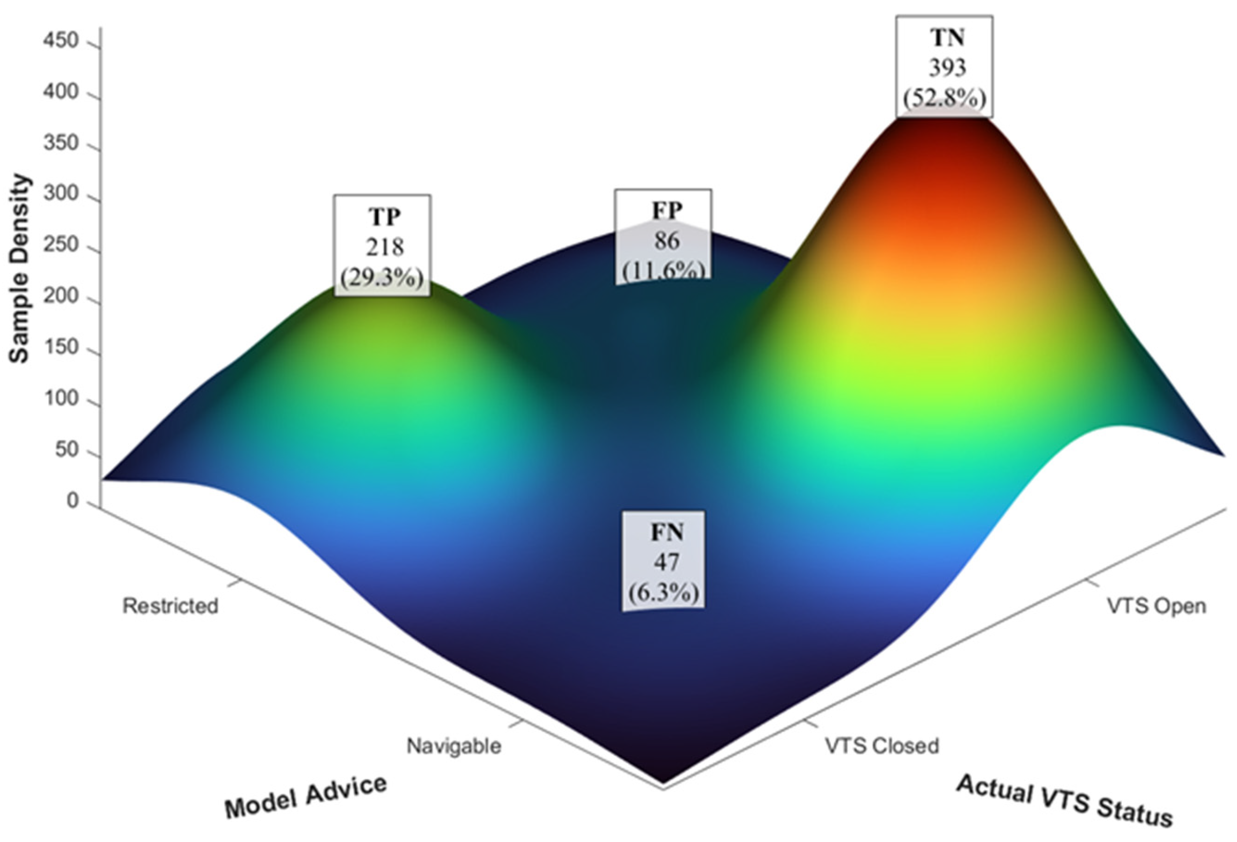
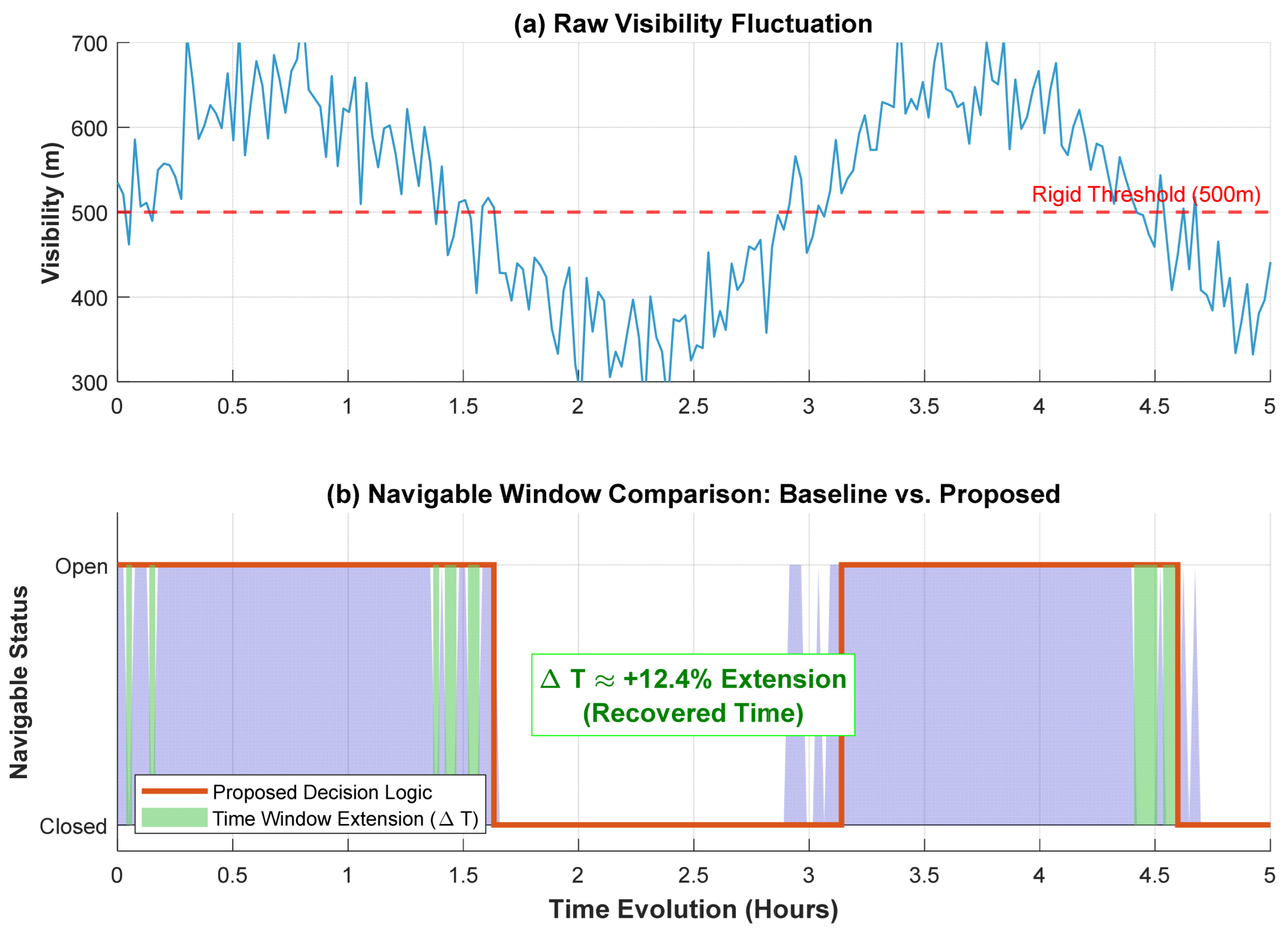
• The proposed Sailability Score achieved 82.1% consistency with actual VTS restriction windows and extended effective navigable time windows by 12.4%, supporting safer and more efficient navigation in fog conditions.

What are the implications of the main findings?

• The simulation findings suggest that UAV-based fog perception can provide reliable real-time environmental awareness for main-route navigation, helping bridge the limitations of conventional radar- and AIS-based monitoring in low-visibility waterways.
• The validated Sailability Score indicates potential for practical deployment in intelligent VTS and smart shipping systems, supporting safer traffic control, more consistent restriction decisions, and more efficient use of navigable time windows under fog conditions.

Abstract

Low-visibility environments induced by sea fog severely constrain the navigational efficiency and safety in narrow waterways, where traditional radar and Automatic Identification Systems (AIS) frequently encounter challenges such as perception blind spots and information lag. To address this critical issue, this study proposes a UAV-based perception and decision-making methodology for main navigational routes in fog, integrating physical priors with unmanned aerial vehicle (UAV) vision. Firstly, a joint physical dehazing and fog-domain adaptive detection network is constructed. This network addresses the overcomes the interference of non-uniform fog through feature-level enhancement, generating a spatio-temporally continuous visibility field and ship probability grids under a bird’s-eye view (BEV). Subsequently, a quantified “Sailability Score” model is established, providing a scientific basis for the dynamic diversion, speed limitation, and safe distance maintenance of main navigational routes. Simulation-based verifications using real-world fog navigation scenarios in the Qiongzhou Strait, coupled with a joint analysis of Vessel Traffic Service (VTS) and AIS data, suggest that at the critical visibility threshold (≤500 m), the proposed method improves the recall rate of long-distance small target detection by approximately 16.2% and reduces the visibility estimation error by 19.3%. Furthermore, the consistency between the proposed Sailability Score and the actual VTS navigation restriction windows reaches 82.1%, exhibiting a conservative preference for safety (i.e., risk preference ratio $\gamma >1$). Additionally, by introducing a temporal anti-jitter mechanism (parameterized by a smoothing window $\Delta t$), the proposed method extends the navigable time window of the main routes by approximately 12.4% while ensuring navigational safety. The simulation results indicate the framework’s potential perception capabilities and engineering applicability, providing reliable technical support for smart shipping and intelligent VTS systems.

1. Introduction

Amid the continuous development of global smart shipping systems, sea fog has emerged as a critical factor that significantly impairs navigational safety and efficiency in narrow waterways [1]. The characteristics of high humidity and intense scattering intrinsic to sea fog lead to the degradation of optical observations, the attenuation of radar signals, and the instability of trajectory recognition. Studies focusing on typical strait regions indicate that ship collision avoidance decision-making and traffic organization under fog navigation conditions are highly susceptible to systemic failures induced by sudden drops in visibility. Ding et al. (2022) conducted observations and simulations of heavy fog events in the Qiongzhou Strait utilizing the WRF model, revealing the nonlinear relationship between local meteorological factors and visibility evolution, thereby providing a dynamic basis for regional fog navigation research [2]. Building upon this, Kim et al. (2023) proposed a data-to-data translation framework for sea fog nowcasting, enabling visibility prediction at a minute-level scale [3]. Yi et al. (2023) utilized geostationary satellite multispectral images to discriminate between sea fog and low clouds, achieving continuous monitoring of the South China Sea and coastal regions [4]. Furthermore, Liu et al. (2024) constructed near-real-time atmospheric and oceanic products for the South China Sea through Himawari-8/9 multi-source inversions, providing fundamental data support for visibility monitoring under fog navigation scenarios [5].

Traditional visibility instruments struggle to meet the requirements of dynamic navigational scenarios; consequently, optical perception and dehazing algorithms have emerged as research hotspots in recent years [6,7]. Yang et al. (2024) systematically reviewed infrared and visible image fusion algorithms, highlighting that multi-scale feature integration and deep learning exhibit superior performance under complex meteorological conditions [8]. Zhu et al. (2019) pioneered a single-image dehazing method based on generative adversarial networks (GANs), achieving significant improvements in preserving texture details and structural consistency [9]. Meanwhile, classic single-image dehazing methods, such as the dark channel prior and color attenuation prior, have provided interpretable baselines for the estimation of transmittance and atmospheric light [10,11,12]. Fu et al. (2024) constructed a hyperspectral dehazing benchmark dataset and designed a deep dehazing model, offering standardized support for the restoration of remote sensing and UAV images in dense fog scenarios [13]. Furthermore, Ma et al. (2022) established a temporal dehazing network by incorporating temporal information, which realized multi-frame fusion and dynamic compensation, thereby enhancing image stability during fog evolution [14]. To further enhance cross-spectral feature integration capabilities, Yang G. et al. (2024) proposed a multi-scale information integration framework, significantly optimizing the fusion performance of infrared and visible images in foggy environments [15].

Foggy environments not only impair visual restoration but also pose a direct threat to the accuracy of ship detection and trajectory tracking. Xie et al. (2024) implemented a highly robust ship detection and tracking system based on LiDAR technology, significantly reducing perception latency [16]. Qu et al. (2023) integrated AIS and visual information, thereby enhancing target recognition consistency in maritime traffic monitoring [17]. Furthermore, Chen et al. (2024) employed an instance association framework to achieve the automatic extraction of video trajectories, providing an algorithmic foundation for continuous ship tracking [18]. Concurrently, focusing on the intelligent analysis of AIS data, Tu et al. (2018) systematically reviewed pattern mining in maritime traffic behavior, offering a theoretical framework for data fusion in smart shipping [19].

With the maturation of unmanned aerial vehicle (UAV) perception platforms, their multimodal fusion perception capabilities under low-visibility conditions have attracted widespread attention [20]. The DSG-Fusion model proposed by Yang X. et al. (2022) utilizes generative networks, exhibiting high robustness in end-to-end infrared and visible image fusion [21]. Pande et al. (2023) achieved the fusion optimization of multimodal remote sensing data through self-supervised learning, thereby reducing reliance on annotations [22]. Regarding safety decision-making, Brandt et al. (2024) constructed a machine learning-based maritime accident prediction model incorporating weather data, improving the accuracy of risk assessment under low visibility [23]. Zhang et al. (2025) proposed a system-driven intelligent decision framework for ship collision avoidance and grounding, enabling adaptive risk assessment in complex environments [24]. Furthermore, from the perspective of reliability, Sánchez et al. (2025) conducted a system-level evaluation of collision avoidance systems, refining the safety control system for intelligent navigation [25].

Beyond 2D perception, 3D reconstruction and situational reasoning hold significant importance in fog navigation scenarios. Qiu et al. (2024) reconstructed the 3D morphology of ships based on Neural Radiance Fields (NeRF), thereby enhancing situational visualization capabilities under complex weather conditions [26]. Regarding image enhancement and feature injection, the MFIFusion model proposed by Dong et al. (2024) utilized a multi-level feature injection mechanism, improving fusion performance under foggy conditions [27]; meanwhile, the UIRGBFuse model proposed by Yi S. et al. (2024) introduced an uncertainty-guided mechanism, reducing the bias in the fusion of infrared and visible features [28]. Wang Z. et al. (2023) accomplished multi-scale fusion optimization through a dual-path residual attention network [29], whereas the WaveFusionNet model developed by Liu R. et al. (2024) integrated multi-scale features with wavelet transforms, further enhancing fusion efficacy in low-contrast environments [30]. Furthermore, research on fog-domain semantic understanding driven by synthetic fog data has provided a conventional benchmark for robustness evaluation in low-visibility scenarios [31].

In summary, while existing studies have significantly advanced sea fog forecasting and multimodal fusion, three critical gaps remain: the separation of visual restoration and target detection leading to physically inconsistent inferences, the spatiotemporal scale mismatch between single-point sensors and UAV perception, and the lack of engineering-deployable quantitative sailability models.

To address these gaps, this study proposes a UAV-based collaborative perception and sailability assessment framework. While the framework incorporates several established modules, their integration addresses the ‘cascading error’ and ‘feature submergence’ problems inherent in traditional decoupled maritime perception pipelines. Unlike existing multimodal systems that treat dehazing and detection as independent tasks, our approach introduces a Physically Consistent Joint Optimization. By utilizing atmospheric scattering parameters as latent anchors that simultaneously constrain both visual restoration and feature extraction, the framework ensures that perception reliability is mathematically coupled with the decision-making logic:

(1) Physically Consistent Joint Optimization: We design a jointly optimized perception architecture where atmospheric scattering parameters derived from a dehazing model are utilized as latent anchors. This physically consistent feature injection mechanism integrates visual restoration and target recognition, replacing traditional independent algorithmic steps.

(2) Spatio-Temporal Mapping: We leverage the UAV’s high-altitude vantage point to transform perspective-distorted visual inputs into spatially consistent 3D probability grids. This “Continuous Field Perception” architecture overcomes the representativeness errors inherent in traditional fixed sensors, establishing a physically consistent basis for navigability assessment that is unconstrained by sea-level geometric limitations.

(3) Quantitative Decision Optimization: We develop a novel Sailability Score model that integrates route diversion, speed limitation, and safe distance maintenance. By incorporating a temporal anti-jitter mechanism, the framework provides stable, real-time decision support for intelligent VTS operations in complex heterogeneous fog.

The findings of this research contribute to the realization of autonomous navigational perception and intelligent VTS decision-making under low-visibility conditions, offering a novel perspective for the safe and efficient transit of strait-type waterways.

2. Materials and Methods

2.1. Problem Description

Sea fog represents a typical high-risk meteorological phenomenon that compromises navigational safety in ports and narrow waterways. Its intrinsic optical scattering characteristics significantly attenuate the perception accuracy of radar and Automatic Identification Systems (AIS), resulting in issues such as trajectory latency, monitoring blind spots, and collision avoidance lag. Traditional shore-based perception systems struggle to maintain stable data links and reliable target recognition during sudden drops in visibility, which severely constrains the operational reliability of smart shipping in low-visibility environments. Particularly in typical semi-enclosed waterways such as the Qiongzhou Strait, days characterized by fog navigation where visibility falls below the critical threshold (e.g., 500 m) account for an average of over 20%. Consequently, navigational safety decision-making relies heavily on manual experience, complicating automated operations.

Furthermore, overcoming these navigational bottlenecks requires more than a simple system-level assembly of existing algorithms. Traditional cascaded perception pipelines often treat visual dehazing and target detection as independent steps, inevitably leading to “cascading errors” where artificial restoration artifacts severely degrade downstream recognition in heterogeneous fog.

While stationary radars or AIS are often limited by sea-level signal attenuation and fixed viewing angles, the UAV acts as a “mobile perception node” from a superior Bird’s-Eye View (BEV). By dynamically aligning visibility gradients with ship trajectories in a unified coordinate system, this framework ensures that navigability quantification is derived from a continuous spatial field rather than discrete, localized extrapolations.

The core of this integration lies in establishing a physically consistent coupling between environmental scattering and spatial perception; by utilizing the inverted transmittance field as a latent physical anchor to dynamically re-weight detection feature channels, the framework mathematically binds perception reliability with decision-making logic.

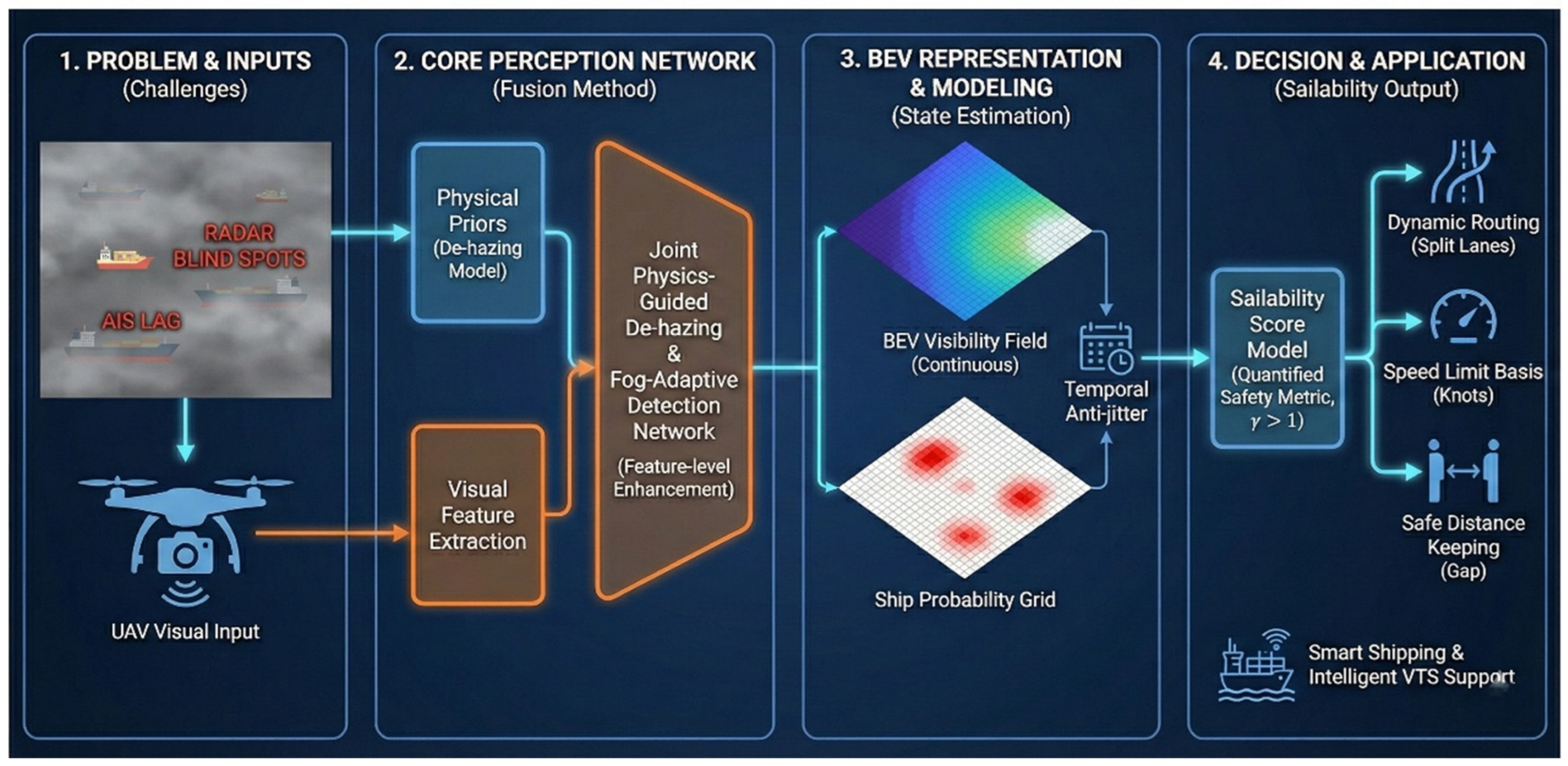
Driven by this physically coupled architecture, this study proposes a UAV-based perception and navigability quantification framework for main navigational routes under fog conditions. Through multi-source information fusion, this framework achieves comprehensive full-process modeling, encompassing physical restoration, target recognition, and navigability assessment. The flowchart of the proposed model is illustrated in Figure 1. Its overall logic comprises three core phases: perception modeling, data calibration, and navigational recommendation generation. Equipped with dual visible light and infrared sensors, the UAV achieves target recognition and trajectory mapping via a “physically consistent dehazing model” and a “fog-domain adaptive target detection” algorithm. Subsequently, visibility grids and ship probability maps are generated under a bird’s-eye view (BEV). Through the “Sailability Score” calculation module, the system outputs recommendations for route diversion, speed limitation, and safe distance maintenance. Model verification relies on lightweight port data—including route centerlines, visibility records, VTS interventions, and lightweight AIS trajectories—to accomplish the alignment and consistency verification of the perception results.

To formulate the problem, the following assumptions are established:

(1) It is postulated that during the study period, the local visibility and fog density exhibit a continuous, differentiable, and monotonically decreasing relationship, which can be approximated as a smooth visibility field $V(x,y,t)$. This assumption is justified by the macroscopic physical characteristics of sea fog in the target waterway, where spatial density variations within the UAV’s localized field of view typically evolve as continuous gradients rather than abrupt, discrete jumps.

(2) The operating altitude $H_d$ of the unmanned aerial vehicle (UAV) remains stable, and the influence of wind field disturbances is negligible, allowing it to be treated as a quasi-static observation platform. This condition is maintained by the UAV’s built-in flight control and stabilization systems, which compensate for routine coastal wind fields to ensure precise spatial tracking.

(3) The imaging noise of the calibrated electro-optical and infrared (EO/IR) dual sensors conforms to a zero-mean Gaussian distribution, and the infrared and visible images possess complementary features within the target area.

(4) During multispectral fusion, the difference in the detection probability of the same target in adjacent frames does not exceed ε, thereby ensuring temporal smoothness and trajectory continuity. This bounded detection variation is strongly justified by the macroscopic kinematic properties of commercial shipping vessels. Given their massive inertia and relatively slow maneuvering speeds, their visual and thermal signatures change marginally within the ultra-short temporal interval (approx. 0.033 s) of the UAV’s 30 fps sampling rate, preventing abrupt feature degradation and ensuring algorithmic tracking stability.

(5) The EO/IR image frames, AIS trajectories, and VTS timelines can be aligned in the time domain via linear interpolation. The validity of this linear alignment is supported by the high temporal resolution of the perception data (30 fps), which is several orders of magnitude higher than the dynamic change rate of shipping vessels.

(6) The geometric morphology of the main navigational route is known and can be projected onto the bird’s-eye view (BEV) coordinate system as a navigable area constraint to calibrate the ship probability distribution.

(7) The Sailability Score is formulated as a linear weighted combination of the visibility term, the target probability term, and the safe distance term (e.g., $S=w_V{S}_V+w_P{S}_P+w_D{S}_D,w_V+w_P+w_D=1$). This linear assumption at the decision level is justified because the underlying non-linear environmental dynamics (e.g., the exponential attenuation of fog) have already been addressed within the individual sub-functions ($S_V$, $S_P$, $S_D$). Consequently, employing a linear synthesis at the final output stage not only maintains the interpretability of the decision logic for VTS operators, but also provides the computational efficiency required for real-time closed-loop control.

(8) A minimized port dataset—comprising the route centerline, visibility records, VTS interventions, AIS trajectories, and fog event lists—is sufficient to support model parameter calibration and verification.

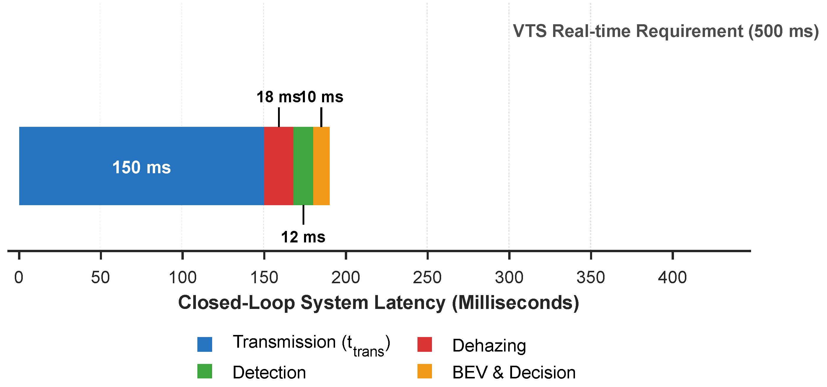
(9) The UAV communication link latency is less than 0.5 s; thus, the observation data is considered to be transmitted in real time, satisfying the requirements of information-driven closed-loop decision support (rather than physical flight control). This sub-second latency is sufficient because the maneuvering response times of vessels and the intervention cycles of Vessel Traffic Service (VTS) are typically measured in minutes, rendering the transmission delay negligible for decision-making.

(10) The model maintains perceptual validity even under extreme fog conditions where visibility is less than or equal to the critical threshold, meaning that the output Sailability Score can predict VTS navigation restriction windows within a margin of error of ±δ.

2.2. Notation

To accurately construct the structured spatio-temporal representation of the navigational environment, specific algorithmic and geometric parameters must be explicitly defined. The generation of the continuous visibility field and the discrete ship probability grid under the Bird's-Eye View (BEV) relies on a set of core parameters. These parameters govern the coordinate transformation from the 2D UAV image plane to the 3D BEV space, determine the spatial resolution of the grids, and establish the boundary conditions for subsequent risk evaluation.

To provide a clear reference for the mathematical modeling and experimental setup, the detailed definitions, symbols, and configured values of the primary parameters utilized in this framework are systematically summarized in

Table 1. Nomenclature and mathematical symbols used in the proposed framework.

Category	Symbol	Description
Time & Weather	$t$	Time of observation or modeling
	$R{H}_t,T_t,P_t$	Relative humidity, air temperature, and atmospheric pressure at time $t$
	$R{H}_0,T_0,P_0$	Humidity, temperature, and pressure under standard reference conditions
	${\rho }_t$	Fog density (mass concentration of liquid droplets per unit volume)
	$a_0,a_1,a_2,a_3$	Regression coefficients of meteorological variables to fog density
Visibility & Optics	$V_t$	Visibility (horizontal visual range) at time $t$
	$V_0$	Critical visibility threshold for safe navigation
	$V_{clear}$	Baseline visibility under clear weather conditions
	$k$	Fog intensity attenuation coefficient
	$I(x,y)$	Observed image (luminance distribution affected by scattering)
	$J(x,y)$	Dehazed image (recovered true radiance)
	$A$	Atmospheric light intensity (global illumination constant)
	$t(x,y)$	Transmittance (proportion of light penetrating the fog medium)
	$\beta$	Scattering coefficient (proportional to fog density)
	${\lambda }_1,{\lambda }_2$	Regularization weights for structural preservation and spectral consistency
	$\varphi ()$	Spectral mapping function for IR and visible image feature alignment
	$I_{\mathrm{VIS}},I_{\mathrm{IR}}$	Visible light and infrared observed images (and their correspondingly recovered true radiances)
Perception & Grids	$V_g(i,j)$	Visibility grid (average visibility in a local BEV region)
	$p_k,{p^{\prime }}_k$	Initial detection confidence and modified detection confidence
	${\alpha }_t$	Fog-domain weight coefficient dynamically adjusting detection intensity
	$\gamma$	$\mathrm{Exponential}\mathrm{adjustment}\mathrm{coefficient}\mathrm{controlling}\mathrm{sensitivity}\mathrm{of}{\alpha }_t$
	${\alpha }_{min},{\alpha }_{max}$	Upper and lower limits of the fog-domain weight
	$P_g(i,j)$	Ship probability grid (probability of target existence)
Sailability Score	$S(i,j)$	Local sailability score integrating visibility, density, and distance
	$f_V,f_P,f_D$	Sub-functions mapping the impacts of visibility, density, and distance
	$w_V,w_P,w_D$	$\mathrm{Weight}\mathrm{coefficients}\mathrm{for}\mathrm{the}\mathrm{three}\mathrm{sub}\text{-}\mathrm{functions}({\displaystyle \sum w_i}=1$)
	$D_g$	Actual safe distance (minimum Euclidean distance between trajectories)
	$D_{safe}$	Safe distance threshold
	$S_{thr}$	Navigability determination threshold (critical value for route navigability)
	$S_{nav}$	Overall sailability score (average of the regional scores)
Evaluation Metrics	$R_{risk}$	Navigational risk degree
	$R_{max}$	Maximum acceptable risk degree
	$Z$	Consistency index (overlap rate between model output and VTS windows)
	$T_{nav}$	Navigable time window (duration for which conditions are satisfied)
	$\Delta R,\Delta E,\Delta T$	Proportional improvements in recall rate, visibility error, and time window
	$T_{smooth}$	Engineering filtering parameter (smoothing window, min)
	$\eta$	Ratio of false positives to false negatives (FP/FN), indicating risk preference
	$F_{sw}$	Switching frequency (number of state switches per unit of time)
	$D_{res}$	Response delay (average lag time to identify sudden localized fog)
	$f_{sys}$	End-to-end system processing frequency (FPS)

. These configured parameters ensure the mathematical consistency and physical alignment of the cross-domain mapping process, serving as the foundational constraints for the Sailability Score calculation in the next stage.

2.3. Fog Intensity Estimation Model

Based on single-station meteorological observation data, a temporal mapping relationship between local fog density and baseline visibility is initially established. The baseline fog density ${\rho }_t$ is determined by relative humidity, air temperature, and atmospheric pressure, which is formulated as:

$${\rho }_t=a_0+a_1{\displaystyle \frac{(R{H}_t-R{H}_0)}{R{H}_0}}+a_2(T_0-T_t)+a_3(P_0-P_t)$$

(1)

The relationship between visibility and fog density satisfies an exponential attenuation model:

$$V_t=V_{clear}{e}^{-k{\rho }_t}$$

(2)

where $V_{clear}$ denotes the baseline visibility under clear weather conditions, and $k$ represents an empirical constant. It is important to note that $V_t$ only reflects the macroscopic temporal trend from shore-based observations. To capture the spatial heterogeneity of patchy fog over the waterway, this macroscopic temporal baseline is used as a prior constraint. By jointly inverting this baseline with the optical transmittance extracted from multiple UAV cruise images, a localized, spatio-temporally continuous visibility field $V(x,y,t)$ is dynamically constructed, thereby providing a precise physical input for the dehazing model.

2.4. Physically Consistent Dehazing Model

Imaging under sea fog conditions can be formulated by the atmospheric scattering equation:

$$I(x,y)=J(x,y)t(x,y)+A(1-t(x,y))$$

(3)

where $I(x,y)$ denotes the observed image, $J(x,y)$ represents the recovered true radiance after dehazing, A is the atmospheric light intensity, and $t(x,y)=e^{-\beta d(x,y)}$ is the transmittance.

By incorporating cross-spectral consistency alongside a smoothness regularization term, the optimization objective function is constructed as follows:

$${\min }_{J,t}\Vert I-Jt-A(1-t){\Vert }_2^2+{\lambda }_1\Vert \nabla J{\Vert }_1+{\lambda }_2\Vert J_{IR}-\varphi (J_{VIS}){\Vert }_2^2$$

(4)

where the squared L2-norm term $\Vert I-Jt-A(1-t){\Vert }_2^2$ denotes the data fidelity constraint (representing the residual of the atmospheric scattering model). The L1-norm term $\Vert \nabla J{\Vert }_1$ is applied to the first-order spatial gradient of the restored image to enforce sparsity for edge preservation. The second L2-norm term $\Vert J_{\mathrm{IR}}-\varphi (J_{\mathrm{VIS}}){\Vert }_2^2$ minimizes the cross-spectral consistency residual between the infrared and the mapped visible features.

To solve this multi-variable optimization problem, an alternating minimization strategy (e.g., ADMM) is utilized to iteratively update the restored radiance $J$ and the transmittance map $t$ until the objective function converges.

Following the joint optimization, both the restored true radiance $J^{*}(x,y)$ and the optimal transmittance map $t(x,y)$ are simultaneously acquired. Since transmittance is physically tied to the scattering coefficient $\beta$, this enables the direct inversion of local visibility:

$$V(x,y)=-{\displaystyle \frac{1}{\beta }}\ln t(x,y)$$

(5)

Subsequently, the visibility grid is generated via regional averaging:

$$V_g(i,j)={\displaystyle \frac{1}{\left|{\Omega }_{ij}\right|}}{\displaystyle \sum _{(x,y)\in {\Omega }_{ij}}V}(x,y)$$

(6)

2.5. Fog-Domain Adaptive Detection and Trajectory Mapping Model

To uniformly represent the detection results at the waterway scale, this study employs a bird’s-eye view (BEV) projection and fuses multi-frame trajectory information utilizing dynamic probabilistic occupancy grids. For related dynamic occupancy grid modeling and real-time inference methodologies, please refer to [32]; a comprehensive review of visual BEV representations and their extensions can be found in [33].

Specifically, we adopt YOLOv8 as the base detection architecture. To integrate the dual-modal inputs, an early-to-middle feature fusion strategy is implemented. The dehazed visible images and the corresponding infrared thermal images are initially processed through parallel convolutional stems to extract modality-specific shallow features. These features are then concatenated along the channel dimension before being fed into the deeper PANet (Path Aggregation Network) neck. This fusion strategy ensures that the complementary thermal signatures compensate for the optical degradation in dense fog before the final bounding box regression. The fused feature sequences are subsequently fed into the detection head, yielding the output target set:

$${\mathcal{O}}_t={\{(b_k,p_k)\}}_{k=1}^{N_t}$$

(7)

To compensate for the recognition degradation under low-visibility conditions, a visibility-correlated weight is introduced: The methodological core of this module is the visibility-correlated weight modulation. By defining the adaptive coefficient $\omega (V)$ as a dynamic function of the real-time visibility field $V(x,y,t)$, the framework achieves a probabilistic re-weighting of feature channels. This provides a theoretical solution to the “feature submergence” problem in non-uniform fog, allowing the detector to proactively increase sensitivity in low-confidence regions based on physical feedback:

$$\alpha (x,y,t)=e^{-\gamma /V(x,y,t)}$$

(8)

To continuously track these dynamically re-weighted targets across sequential frames, multi-object temporal association is accomplished via a weighted Hungarian algorithm. Specifically, the association cost matrix is computed based on the Intersection over Union (IoU) of the bounding boxes and the Euclidean distance between the target center points in the BEV plane:

$$\mathcal{T}={\left\{{\tau }_m\right\}}_{m=1}^M,{\tau }_m=\{b_{m,t_0},\dots ,b_{m,t_n}\}$$

(9)

The trajectories are subsequently projected into the BEV coordinate system to generate the ship probability grid:

$$P_g(i,j)={\displaystyle \frac{1}{\left|{\Omega }_{ij}\right|}}{\displaystyle \sum _{{\tau }_m\cap {\Omega }_{ij}\ne \varnothing }{p}_m^{\prime }}$$

(10)

2.6. Sailability Score and Risk Quantification Model

Building upon the visibility grids and ship probability grids, the local sailability score is defined as follows:

$$S(i,j)=w_V{f}_V(V_g(i,j))+w_P{f}_P(P_g(i,j))+w_D{f}_D(D_g(i,j)),w_V+w_P+w_D=1$$

(11)

where $f_V(V_g)$,  $f_P(P_g)$, and $f_D(D_g)$ denote the normalized sub-functions for visibility, probability, and distance, respectively, which are formulated as:

$$\begin{array}{l}{f}_V(V_g)=1-e^{-V_g/V_0},\\ f_P(P_g)=1-P_g,\\ f_D(D_g)=\min (1,D_g/D_{\mathrm{safe}})\end{array}$$

(12)

Consequently, the overall sailability score is calculated as:

$$S_{\mathrm{nav}}={\displaystyle \frac{1}{N_g}}{\displaystyle \sum _{i,j}S}(i,j)$$

(13)

Navigability is affirmed when the condition $S_{\mathrm{nav}}\ge S_{\mathrm{thr}}$ is satisfied.

Furthermore, the navigational risk degree is quantified as:

$$R_{\mathrm{risk}}=1-S_{\mathrm{nav}}$$

(14)

Such quantified collision risk metrics driven by traffic data have been extensively investigated and applied in maritime safety assessments [34,35]. The consistency of the proposed model is evaluated by its overlap rate with the actual Vessel Traffic Service (VTS) navigation restriction windows, which is expressed as:

$$Z={\displaystyle \frac{T_{\mathrm{overlap}}}{T_{\mathrm{total}}}}\times 100\%$$

(15)

2.7. Dynamic Feedback and Time Window Optimization Model

To establish an adaptive decision-support loop for Vessel Traffic Service (VTS)—focusing on high-level traffic regulation rather than microscopic UAV flight guidance, the navigable time window function is formulated as follows:

$$T_{\mathrm{nav}}={\displaystyle {\int }_{t_0}^{t_1}\mathbb{I}}(S_{\mathrm{nav}}(t)\ge S_{\mathrm{thr}})dt$$

(16)

The optimization objective is to maximize the navigable time window:

$${\max }_{{\alpha }_t,w_V,w_P,w_D}{T}_{\mathrm{nav}}$$

(17)

This is subject to the following constraints:

$$\left\{\begin{array}{ll}{V}_t\ge V_0\hfill & \hfill \\ R_{\mathrm{risk}}(t)\le R_{\max }\hfill & \hfill \\ {\alpha }_t\in [{\alpha }_{\min },{\alpha }_{\max }]\hfill & \hfill \end{array}\right.$$

(18)

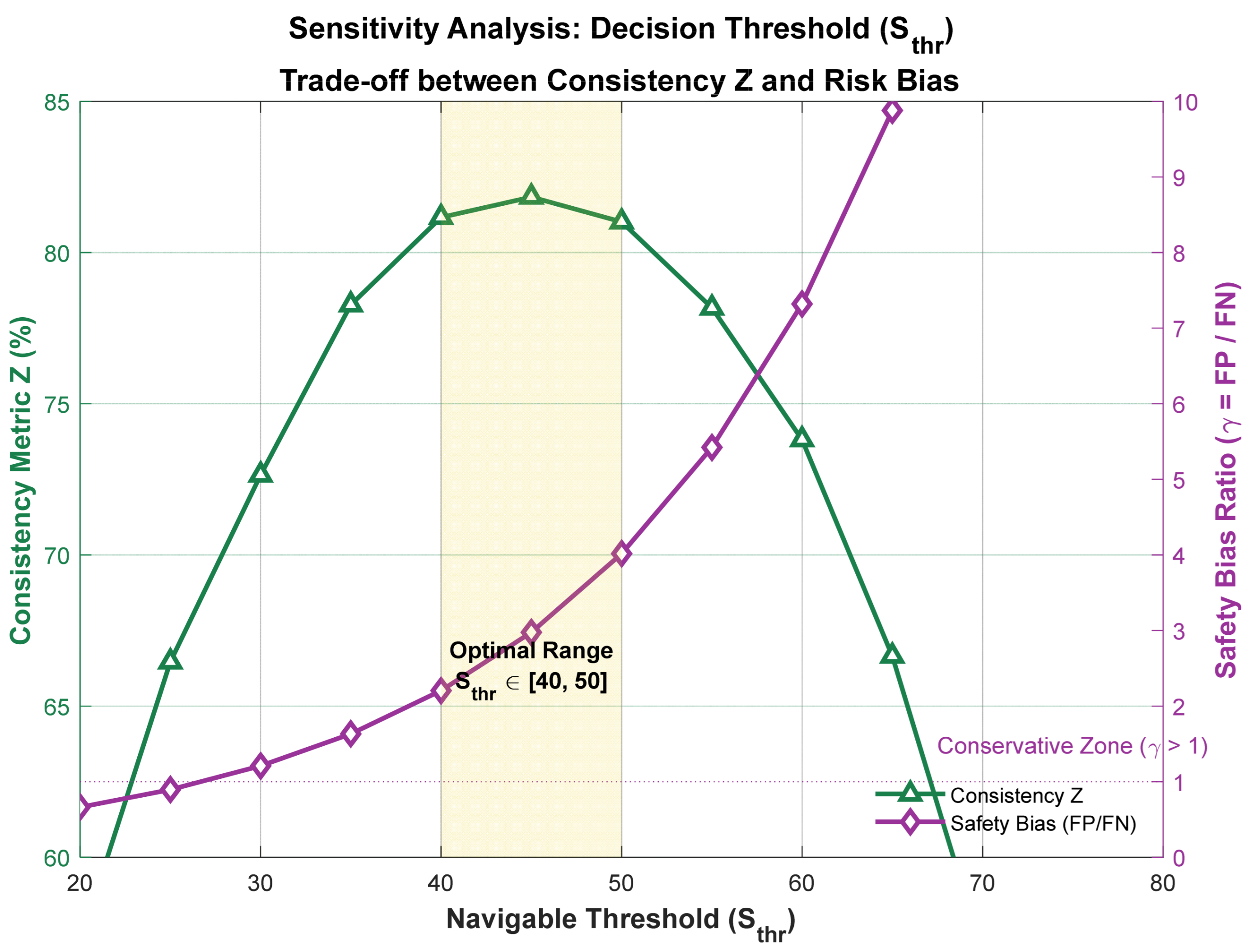
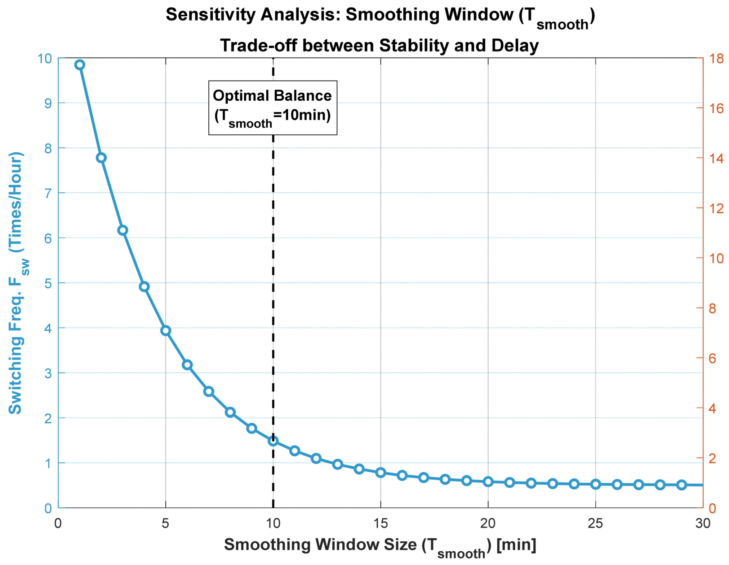
Adaptive feedback regulation of the system is accomplished by iteratively adjusting the detection weight limits (${\alpha }_{\min },{\alpha }_{\max }$) alongside the scoring weights ($w_V,w_P,w_D$). Given that the objective function (Equation (17)) incorporates non-differentiable discrete thresholds (Equation (16)), the optimization of these hyperparameters is executed via a data-driven offline grid search over the historical training dataset. Specifically, the sailability scoring weights ($w_V,w_P,w_D$) are constrained by $w_V+w_P+w_D=1$ and optimized using a grid search step size of 0.05. The optimal combination ($w_V=0.4,w_P=0.4,w_D=0.2$) was empirically selected based on maximizing the consistency index $Z$ against the actual VTS control timelines. Concurrently, the fog-domain adaptive weight limits (${\alpha }_{\min },{\alpha }_{\max }$) were tightly bounded to the interval $[1.0,3.0]$. This explicit bounding prevents gradient explosion and excessive feature suppression during dynamic channel re-weighting, ensuring stable target recall even under severe patchy fog conditions. By solving this detailed optimization problem offline, the system dynamically balances strict safety margins with real-time operational efficiency during online deployment. The system’s performance metrics include $\Delta R,\Delta E,Z,\Delta T$, which, respectively, quantify the proportional improvement in the recall rate of small targets, the proportional reduction in visibility estimation error, the consistency with VTS interventions, and the proportional extension of the navigable time window.

To summarize the implementation logic of the proposed framework and bridge the gap between individual mathematical models, the complete process from environmental perception to navigability decision-making is integrated into Algorithm 1.

Algorithm 1: UAV-based Collaborative Perception and Sailability Assessment (UCPSA).

Input: Dual-modal UAV sequences ($I_{\mathrm{VIS}},I_{\mathrm{IR}}$); Real-time meteorological data $M(H,T,P)$; Route spatial constraints; Risk preference $\eta$ and smoothing window $T_{smooth}$. Output: Sailability Score ($S_{nav}$); Navigable Time Window ($T_{nav}$); Dynamic Control Recommendations.         1. Initialization: Synchronize and align $I_{\mathrm{VIS}}$ and $I_{IR}$ frames; Set initial weights $w_V,w_P,w_D$.         2. Macroscopic State Estimation:         Calculate global fog density ${\rho }_0$ and temporal baseline visibility $V_t$ from $M(H,T,P)$ (Equations (2) and (3)).         3. Physical-Prior Perception Processing:         Image Restoration: Execute joint dehazing to acquire restored radiance $J$ and transmittance $t(x,y)$ via ADMM solver (Equation (4)).         Field Construction: Invert the scattering coefficient $\beta$ to generate the continuous visibility field $V(x,y,t)$ (Equations (5) and (6)).         4. Adaptive Detection & Mapping:         Calculate fog-domain adaptive weight ${\alpha }_t$ based on local $V(x,y)$ (Equation (8)).         Perform multi-object association and tracking via weighted Hungarian algorithm (Equation (9)).         Project trajectories to BEV to generate ship probability grid $P_g(i,j)$ (Equation (10)).         5. Sailability Quantification:         Evaluate normalized sub-functions $f_V,f_P,f_D$ for each grid (Equation (12)).         Compute local score $S(i,j)$ and aggregate to obtain overall $S_{nav}$ (Equations (11) and (13)).         6. Decision Optimization:         Apply temporal anti-jitter filtering via $T_{smooth}$ to calculate stable $T_{nav}$ (Equation (16)).         Refine ${\alpha }_t$ and scoring weights $w_V,w_P,w_D$ via offline grid search (Equation (17)).         7. Return $S_{nav}$ and real-time navigation recommendations.

3. Experimental Design and Data Validation

3.1. Overall Simulation Scheme

To verify the feasibility and accuracy of the UAV-based perception method for main navigational routes under typical low-visibility environments, a simulation-based experimental scheme was designed using historical data from the Qiongzhou Strait region. The objective of the simulation is to systematically evaluate the reliability of the proposed model in visibility estimation, trajectory recognition, and Sailability Score calculation through a coupled comparison between UAV perception results and multi-source data.

As a typical narrow shallow-water channel in China, the Qiongzhou Strait is significantly affected by winter monsoons and land–sea temperature gradients. Consequently, sea fog events in this region are characterized by high frequency, temporal concentration, and drastic variations, making it a representative area for validating low-visibility navigational routes. In accordance with the Qiongzhou Strait Ship Routing System and actual Vessel Traffic Service (VTS) control standards, this study establishes the critical visibility threshold for navigational safety at $V_0$ = 500 m. This value serves as the fundamental constant for subsequent model evaluation and threshold analysis.

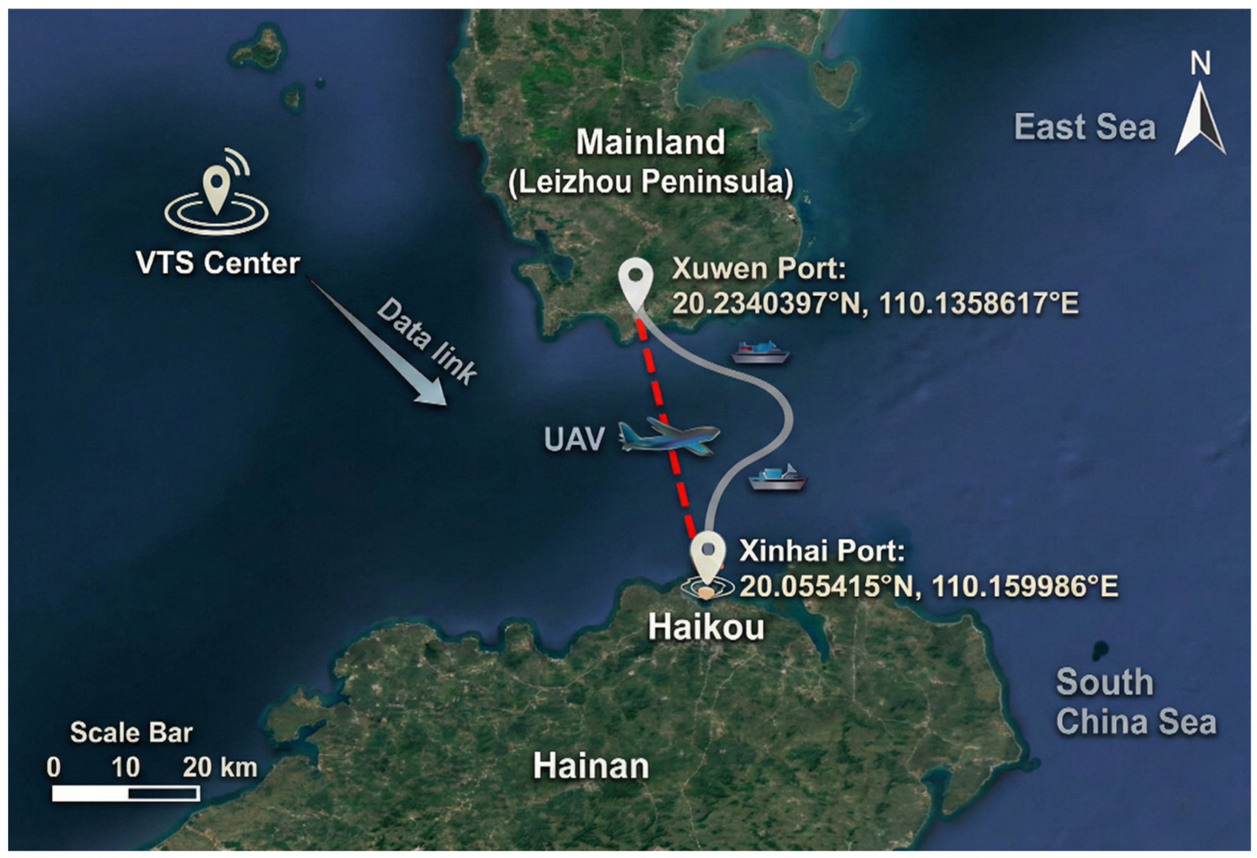
Although radar and Automatic Identification System (AIS) technologies play a crucial role in maritime safety, their limitations persist under complex, low-visibility meteorological conditions. The effectiveness of radar technology is significantly compromised during fog or strong winds, as signal attenuation impairs the accurate identification of long-distance or low-reflection targets. Furthermore, since AIS relies on active signal broadcasting from ships, it is constrained by the attenuation of electromagnetic wave propagation; particularly in foggy weather, the effective reception range of AIS signals is substantially diminished. In this study, the main navigational route of the Qiongzhou Strait is initially selected as the experimental spatial framework ([DATA1]). The coordinates of the main route are extracted from official ship routing system data and standardized into the WGS-84 coordinate system, thereby forming the route centerline dataset required for the experiment. Figure 2 illustrates the geographical scope of the experimental area, the alignment of the main route, key intersection locations, and the settings of the UAV observation paths, serving as a spatial reference for subsequent data collection and alignment.

Under this research framework, the unmanned aerial vehicle (UAV) executes low-altitude observation missions along the main navigational route on typical fog navigation days, acquiring dual-channel electro-optical and infrared (EO/IR) images. The observation times are meticulously aligned with fog event records ([DATA2]) to ensure that the experiment comprehensively covers various visibility levels (L0/L1/L2). Concurrently, minute-level visibility records from port meteorological stations ([DATA3]) are utilized to calibrate the model’s visibility inversion, while lightweight AIS trajectories ([DATA5]) are employed to validate the ship probability grids generated by the trajectory mapping module. Furthermore, the calculated Sailability Score is evaluated for consistency against the Vessel Traffic Service (VTS) control timeline ([DATA4]), thereby verifying the model’s practical reference value in assisting navigational decision-making.

The experimental period spans the early mornings (04:00–09:00) from January to March, a high-incidence season for sea fog, while the spatial scope encompasses the main navigational route and an area extending approximately 2 nautical miles on both sides. All data sources are standardized to the WGS-84 coordinate system [36] and the UTC+8 time standard, ensuring the alignment of UAV imagery, meteorological data, AIS trajectories, and VTS control records within a unified spatiotemporal framework.

Simulation Tasks and Data Collection Workflow

(1)

UAV Flight Path Design

The core of the simulation task lies in designing a scientifically sound flight path to ensure that the unmanned aerial vehicle (UAV) can cover the main navigational route of the Qiongzhou Strait and an area extending approximately 2 nautical miles on both sides. This is particularly crucial on typical fog navigation days to accurately acquire data under varying visibility conditions. The design of the flight path adheres to the following principles: first, ensuring the longitudinal and lateral representativeness of the route; second, covering critical periods of fog occurrence; and third, providing sufficient sample data.

Specifically, based on the main route of the Qiongzhou Strait, and taking into account the geographical features, meteorological conditions, and navigational safety requirements of the waterway, a “U-shaped trajectory + cross-sectional traverse” mode was designed. During each simulated flight mission, the route is scheduled to be divided into multiple regional cross-sections. The UAV hovers over each cross-section for 10–15 s to acquire high-resolution images, with a particular focus on capturing visibility variations during the fog peak, fog valley, and transition phases. Furthermore, all collected visibility data are calibrated against the real-time visibility data provided by port meteorological stations, thereby improving the accuracy and stability of the model’s output. During the flight, the shortest route between cross-sections is selected to minimize non-productive flight time and ensure the acquisition of time-series data regarding visibility evolution.

(2)

Temporal Scheduling

The temporal scheduling of the experiment was specifically designed to target the high-incidence periods of sea fog. Based on local meteorological characteristics, flight missions were primarily scheduled during the peak fog season spanning from December to March of the subsequent year. Particular emphasis was placed on encompassing two critical periods: the early morning (05:00–08:00) and the formation phase of advection fog (16:00–19:00), aiming to capture the complete evolutionary process of visibility from light mist to dense fog and its subsequent dissipation. Throughout the entire simulation experiment, data acquisition tasks were executed within these designated daily time windows, thereby ensuring that the multiple data collection sessions comprehensively encompassed typical fog scenarios under diverse meteorological conditions.

(3)

Mission Execution Procedures

During each simulated flight mission, a fixed-route flight mode is employed to ensure that data acquisition follows the pre-programmed path. The unmanned aerial vehicle (UAV) utilizes a GPS navigation system during flight to ensure precise trajectory tracking, complying with port airspace management regulations and Visual Line of Sight (VLOS) standards [37]. Throughout the mission, data acquisition and flight control are synchronously executed by the onboard flight control system and the UAV ground control station (GCS), thereby ensuring operational stability and safety.

The duration of each simulated flight mission is approximately 20 min in the virtual environment. All flight data generated during each mission—including sensor outputs, flight attitude information, and image data—are subjected to timestamping and attitude synchronization on the onboard terminal, ensuring the reliability of subsequent data analysis.

(4)

Hardware Configuration and Parameter Settings

To ensure the reproducibility of the experiment and the comparability of data across multiple flight sessions, the specific hardware platform and operational parameters are defined. The simulated aerial perception platform is modeled upon an industrial-grade UAV (DJI Matrice 300 RTK, SZ DJI Technology Co., Ltd., Shenzhen, China), assuming a payload of a stabilized EO/IR dual-sensor (Zenmuse H20T, SZ DJI Technology Co., Ltd., Shenzhen, China). The electro-optical sensor operates with a focal length of 31.7 mm and a resolution of 3840 × 2160, while the infrared thermal sensor captures thermal radiation in the 8–14 μm spectral band. The flight altitude is maintained between 150 and 250 m. The sampling frame rate is set at 30 fps to ensure the capture of sufficient details, and a time-synchronized triggering mechanism is employed to ensure temporal consistency between the dual-modal imagery and sensor flight logs.

Furthermore, all algorithmic training and real-time inference validations were conducted on a high-performance computing workstation. The hardware environment comprises an Intel Core i9-13900K processor (Intel Corporation, Santa Clara, CA, USA) and an NVIDIA GeForce RTX 4090 GPU (NVIDIA Corporation, Santa Clara, CA, USA) with 24 GB of VRAM. For the detection configuration, the baseline network (YOLOv8) and the proposed fog-domain adaptive detection network were configured with an input image resolution of 640 × 640. The network was optimized using the AdamW optimizer (implemented in PyTorch, Meta Platforms, Inc., Menlo Park, CA, USA) with an initial learning rate of 0.001, and the intersection-over-union (IoU) threshold for Non-Maximum Suppression (NMS) was set to 0.5 to accommodate the tracking of densely distributed small targets in foggy conditions.

To provide a transparent and highly reproducible overview of the experimental setup, the complete implementation configurations—encompassing hardware platforms, sensor specifications, model hyperparameters, dataset partitioning, and evaluation protocols—are systematically summarized in

Table 2. Detailed specifications of the experimental hardware and software platform.

Category	Parameter/Item	Specification/Value
Hardware Platform	UAV Platform	DJI Matrice 300 RTK (SZ DJI Technology Co., Ltd., Shenzhen, China)
	Computing Workstation	Intel Core i9-13900K (Intel Corporation, Santa Clara, CA, USA), NVIDIA GeForce RTX 4090 (24 GB VRAM) (NVIDIA Corporation, Santa Clara, CA, USA)
Sensor & Data	Payload Sensor	Zenmuse H20T (Dual EO/IR Stabilized Gimbal) (SZ DJI Technology Co., Ltd., Shenzhen, China)
	Optical Resolution & FOV	3840 × 2160, Focal length: 31.7 mm
	Thermal Specification	Spectral band: 8–14 μm
	Sampling Rate	30 fps (time-synchronized triggering)
Model Settings	Perception Baseline	YOLOv8 + Physical-Prior Feature Injection (v8.0, Ultralytics, Los Angeles, CA, USA)
	Input Resolution	640 × 640 pixels
	Optimizer & Learning Rate	AdamW, Initial LR = 0.001
	NMS IoU Threshold	0.5
Data Split	Total Dataset Coverage	January 2025–March 2025 (Early morning, 04:00–09:00)
	Data Split Ratio Core Evaluation Set	Training (80%), Validation (10%), Testing (10%) 1–31 January 2025 (744 h continuous validation)
Evaluation Protocol	Visibility Inversion Metrics	Mean Absolute Error (MAE), Root Mean Square Error (RMSE)
	Target Detection Metric	Recall Rate (focused on long-distance micro-vessels)
	Decision Consistency	Overlap Rate (Z), Sailability Score (Snav)

.

Dataset Annotation and Training Implementation:

To ensure scientific reproducibility, the dataset annotation and model training procedures were standardized. During the annotation process, the EO/IR image pairs were manually annotated with bounding boxes for vessels. To prevent false positives/negatives in dense fog, the visual annotations were cross-referenced and verified against synchronous AIS coordinates. As specified in Table 2, the dataset was partitioned into training (80%), validation (10%), and testing (10%) subsets. The network was trained in a two-stage procedure. First, the physically consistent dehazing module was pre-trained using the composite loss function defined in Equation (4), which balances $L_1$ gradient sparsity and $L_2$ cross-spectral consistency. Subsequently, the entire perception pipeline was fine-tuned end-to-end. The global loss implementation for this stage was a weighted sum of the dehazing reconstruction loss and the YOLOv8 detection losses (incorporating CIoU for bounding box regression and Distribution Focal Loss for classification). Training was executed on the RTX 4090 GPU for 150 epochs with a batch size of 16, utilizing an early stopping mechanism based on validation loss to prevent overfitting.

Comparison and Calibration of Data During Fog Peak, Fog Valley, and Transition Phases:

To comprehensively evaluate the performance of the model under varying visibility conditions, the experiment specifically focuses on data acquisition and calibration during three typical periods: the fog peak, fog valley, and transition phases.

Fog Peak Phase: This represents the period of minimum visibility, typically occurring when the sea fog is at its most severe. During this phase, the model is required to fully leverage its capabilities in dehazing and fog intensity estimation. The experiment evaluates the model’s predictive accuracy for extremely low visibility by comparing the visibility data generated by the model with the observation values from meteorological stations. In this phase, the analysis focuses on whether the model can accurately reflect instantaneous visibility variations and its performance within the central region of the fog body.

Fog Valley Phase: The fog valley is the phase where visibility gradually recovers, typically occurring during the dissipation process of the fog. During this phase, the model’s dehazing efficacy and its responsiveness to visibility variations are of paramount importance. By comparing the model outputs with actual observation data, the stability of the model in a rapidly changing visibility environment is further verified.

Transition Phase: This phase constitutes the transitional process of fog formation and dissipation, characterized by drastic fluctuations in visibility. At this juncture, the model’s reaction speed and predictive accuracy are the focal points of investigation. Through a point-by-point comparison between the model outputs and the observation data from port meteorological stations, the model’s prediction capability for the fog edge regions and its responsiveness to sudden changes are evaluated.

These phase-based comparisons evaluate the model’s stability in dynamic environments, establishing a foundation for subsequent trajectory mapping and Sailability Score analyses.

3.2. Data Sources and Processing Workflow

3.2.1. Data Sources and Acquisition Methods

To ensure the scientific validity and reproducibility of the simulation validation, this study constructs a unified validation database based on multi-source heterogeneous data under typical fog navigation scenarios. The data system comprises five core components: route geometry, fog event records, meteorological observations, traffic control, and ship trajectories, corresponding to [DATA1]–[DATA5], respectively. These components collectively form a “spatial-temporal-shipping” three-dimensional data support framework.

To clarify the data structure and address the multi-source references,

Table 3. Comprehensive implementation details of the UAV-based perception and evaluation framework.

Dataset	Source/Provider	Resolution/Frequency	Application in Experiment
[DATA1] Route Centerline	China Maritime Safety Administration	Static Geometry	Defines spatial constraints for BEV mapping
[DATA2] Fog Events	Port Meteorological Observatory	Event-based (L0/L1/L2)	Guides temporal scheduling of UAV missions
[DATA3] Visibility Records	Shore-based Meteorological Stations	Minute-level	Calibration baseline for visibility inversion
[DATA4] VTS Timelines	Qiongzhou Strait VTS Center	Real-time events	Ground truth for decision consistency analysis
[DATA5] AIS Trajectories	Coastal AIS Broadcasting Stations	2 min resampling	Validation reference for ship probability grids

summarizes the specific datasets, their temporal/spatial resolutions, and their designated applications in the validation process.

(1)

[DATA1] Centerline of the Main Navigational Route in the Qiongzhou Strait

Source: Publicly available navigational route data published by the Maritime Safety Administration of China. This dataset contains the spatial coordinates of the main route in the Qiongzhou Strait.

Acquisition Method: The route centerline data are extracted from official nautical charts (Chart Nos.: 01103, 88001, and 3315) provided by the Maritime Safety Administration. Subsequently, these data are standardized into the WGS-84 coordinate system to ensure spatial consistency with other data sources, such as Automatic Identification System (AIS) trajectories and Vessel Traffic Service (VTS) navigation restriction data.

Preprocessing Procedure: The route centerline data are subjected to a data cleaning process to eliminate invalid points, thereby ensuring the continuity and consistency of the spatial data. All geometric data are uniformly unified into the WGS-84 coordinate system, and temporal synchronization alongside spatial alignment is conducted to ensure spatiotemporal consistency with the other heterogeneous datasets.

(2)

[DATA2] Fog Event List

Source: The fog event data are primarily derived from long-term observations conducted by the port meteorological observatory of the Qiongzhou Strait, supplemented by relevant historical data from the Statistical Report on Sea Fog in the South China Sea. These data provide specific descriptions of fog events for the study, encompassing elements such as start and end times, visibility, and weather types.

Acquisition Method: The data are acquired via real-time observation equipment at the meteorological observatory and combined with multi-year meteorological records to ensure comprehensive coverage of typical sea fog events. Historical data can be accessed through public meteorological data platforms, observatories, and specialized meteorological databases.

Preprocessing Procedure: All temporal data undergo a standardization process, being uniformly converted to the UTC+8 time standard to ensure formatting consistency. The visibility levels of the events (L0, L1, and L2) are delineated based on actual observation data and classified according to varying visibility ranges. To ensure data completeness, missing values are imputed utilizing interpolation methods, thereby ensuring that the dataset is aligned with other multi-source data.

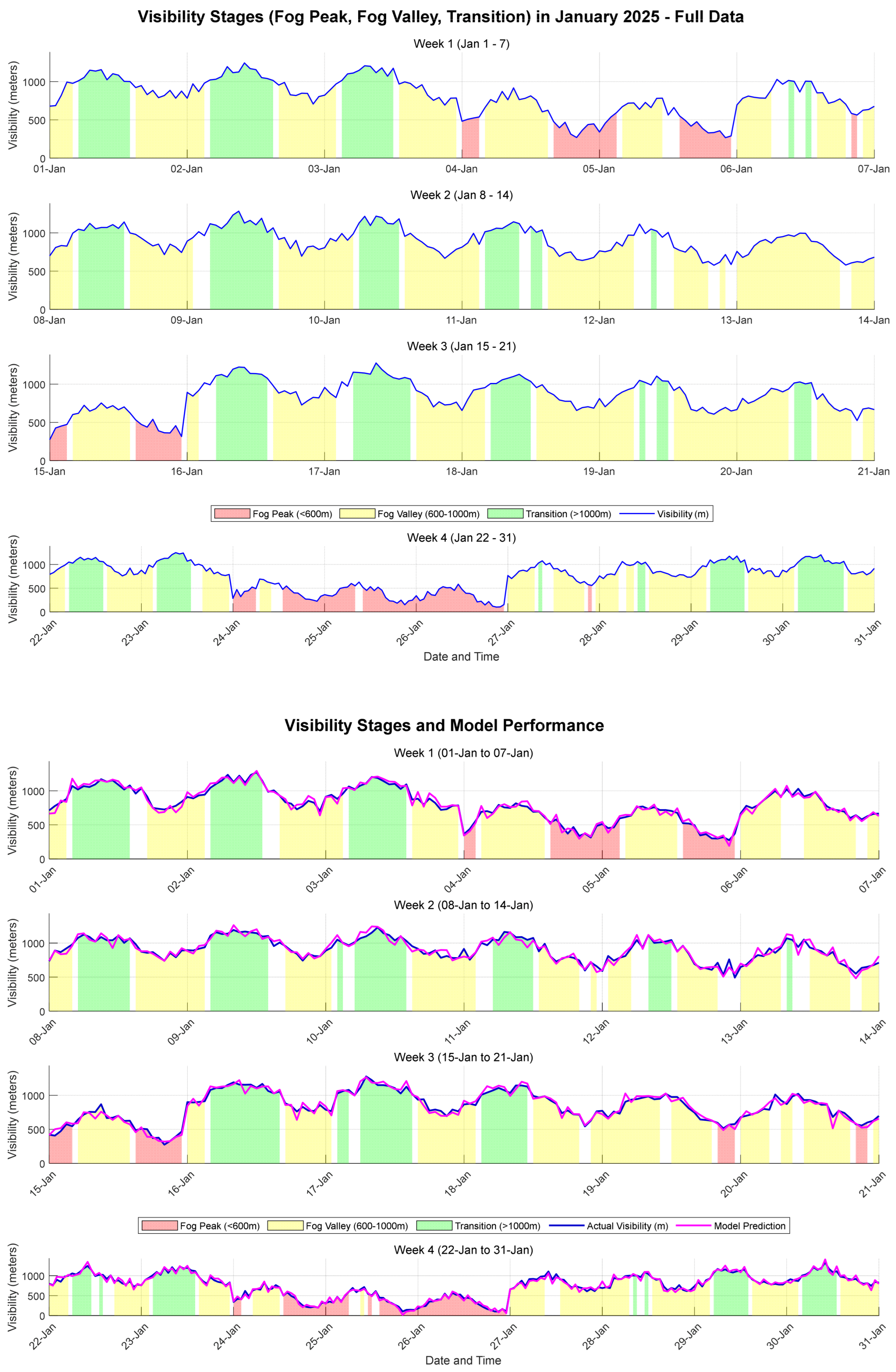
In this study, the visibility data are categorized into three distinct phases: the fog peak, fog valley, and transition phases. Each phase corresponds to a specific visibility range, facilitating a more rigorous evaluation of the model’s performance under varying visibility conditions. Specifically, the fog peak phase is defined by visibility of less than 600 m, primarily corresponding to the period of the densest sea fog; the fog valley phase covers a visibility range from 600 to 1000 m, typically occurring as the fog gradually dissipates; the transition phase is characterized by visibility exceeding 1000 m, indicating relatively clear weather conditions. Figure 3 illustrates the delineation of these three phases, where the green region represents the transition phase, the yellow region denotes the fog valley phase, and the red region indicates the fog peak phase. Through this phase-based categorization, the dynamic variations of data under different visibility conditions can be clearly observed in the experimental dataset.

(3)

[DATA3] Single-Station Visibility Records

Source: The data are sourced from port meteorological stations near the Qiongzhou Strait, primarily providing minute-level visibility observation data. These data are utilized to calibrate the visibility values output by the model.

Acquisition Method: The visibility records from the meteorological stations are obtained through collaboration between the port administration and the meteorological bureau, and are recorded in real-time by on-site equipment. The data possess high spatiotemporal resolution, ensuring their applicability in practical operations.

Preprocessing Procedure: The observation data are denoised, and intermittently missing visibility values are imputed using adjacent-point interpolation.

(4)

[DATA4] Vessel Traffic Service (VTS) Measure Timeline

Source & Acquisition: Acquired from the Qiongzhou Strait VTS center, these data encompass continuous records related to waterway traffic control, particularly traffic restriction, reopening, and warning measures implemented under low-visibility or other adverse weather conditions.

Acquisition Method: The data are collected via the port’s automated traffic management system and integrated with historical traffic control data, ensuring the coverage of multiple fog events and traffic restriction records under various weather conditions over the past few years. These data can be accessed and acquired through navigational warnings, VTS system interfaces, and port regulatory platforms.

Preprocessing Procedure: During the preprocessing phase, all raw control records are aligned according to timestamps and formatted to ensure synchronous analysis with the Sailability Score data output by the model.

(5)

[DATA5] Lightweight AIS Trajectories

Source: The AIS trajectory dataset is provided by public AIS broadcasting stations along the Chinese coast. The Automatic Identification System (AIS) is a global ship tracking system that facilitates the monitoring of dynamic information—such as vessel position, speed, and heading—by automatically broadcasting navigational data. In this study, an anonymized subset of AIS trajectories is utilized, focusing exclusively on the primary shipping vessels navigating the Qiongzhou Strait.

Acquisition Method: The data are acquired via the automated receiving systems of public AIS broadcasting stations. Following preliminary processing, the records encompass fields including the Maritime Mobile Service Identity (MMSI) number, timestamp, latitude and longitude coordinates, Speed Over Ground (SOG), and Course Over Ground (COG). These data document the trajectories of vessels transiting the Qiongzhou Strait, capturing the dynamic variations of ships under foggy weather conditions.

Preprocessing Procedure: To ensure data smoothness, the AIS data are subjected to Kalman filtering, eliminating noise and smoothing the trajectories. Subsequently, the data are resampled at a 2 min frequency and converted into a format compatible with MATLAB (R2023a).

3.2.2. Uncertainty and Limitations of Validation Baselines

While the multi-source dataset ([DATA1]–[DATA5]) provides a comprehensive reference for model validation, it is essential to acknowledge the inherent uncertainties within these “pseudo-ground truth” sources. First, single-station visibility records [DATA3] are point-based measurements that often fail to capture the intense spatial heterogeneity of sea fog across the entire strait; thus, discrepancies between the UAV-derived field and station data may stem from localized fog patches rather than algorithmic error. Second, AIS trajectories [DATA5] are subject to intermittent signal latency and positioning drift (typically 5–10 m) induced by multi-path scattering in high-humidity fog environments. Third, VTS measure timelines [DATA4] are fundamentally driven by human expert experience. There is an inherent “cognitive lag” between the physical onset of dense fog and the official issuance of restriction commands, meaning the VTS window represents a regulatory threshold rather than an instantaneous physical state. By recognizing these limitations, the consistency evaluation in this study aims to demonstrate “operational alignment” rather than absolute physical identity.

3.3. Model Operation and Validation Methods

The operation of the model comprises three primary modules: perception processing, spatial mapping, and navigability evaluation. The UAV-acquired EO/IR images undergo luminance normalization and joint physical dehazing to restore radiance and extract vessel trajectories, bypassing the contrast degradation inherent in raw foggy inputs.

In the spatial mapping phase, the model employs a detection module to extract the spatiotemporal trajectories of vessels, converting them into a standard coordinate system representation via temporal synchronization and spatial projection. All detection results are uniformly transformed into a bird’s-eye view (BEV) perspective, generating a fixed-scale visibility field and a ship probability grid. The visibility field illustrates the visible distance within the region across different times, while the ship probability grid is generated utilizing the Kernel Density Estimation (KDE) method, which integrates ship detection density and confidence to produce a probability distribution map of vessel occurrences at various locations.

The validation methodology of the model encompasses the quantitative evaluation of three core modules: visibility estimation, trajectory mapping, and navigability evaluation. Regarding visibility estimation, the model’s outputs are compared against the minute-level visibility data provided by port meteorological stations. Metrics such as Mean Absolute Error (MAE) and Root Mean Square Error (RMSE) are utilized to assess the model’s error performance under varying fog intensities.

Visibility Estimation Error Evaluation

To quantify the error of the model, this study employs two widely adopted error evaluation metrics: Mean Absolute Error (MAE) and Root Mean Square Error (RMSE). By conducting a point-by-point comparison between the visibility data output by the model and the actual visibility records from port meteorological stations, the calculation formulas are established as follows:

(1)

Mean Absolute Error (MAE):

$$\mathrm{MAE}={\displaystyle \frac{1}{N}}{\displaystyle \sum _{i=1}^N|}{V}_{\mathrm{model}}(i)-V_{\mathrm{obs}}(i)|$$

(19)

where $V_{\mathrm{model}}(i)$ represents the visibility output of the model at the i-th time point, $V_{\mathrm{obs}}$ denotes the actual observation data, and N is the total number of data points compared.

(2)

Root Mean Square Error (RMSE):

$$\mathrm{RMSE}=\sqrt{{\displaystyle \frac{1}{N}}{\displaystyle \sum _{i=1}^N{\left(V_{\mathrm{model}}(i)-V_{\mathrm{obs}}(i)\right)}^2}}$$

(20)

This metric calculates the root mean square difference between the model-estimated visibility and the actual observed values, thereby reflecting the overall error of the model across different time points.

A comparison of the results reveals that the model can accurately track the actual measured data during visibility variations, exhibiting minor errors particularly during the fog peak and fog valley phases. However, during the transition phase characterized by drastic visibility fluctuations, the model exhibits slight underestimations or overestimations, primarily concentrated in the transitional regions at the fog edges. The calculations of MAE and RMSE under varying visibility and fog conditions indicate that the model yields smaller MAE and RMSE values (i.e., lower errors) under normal visibility conditions (e.g., L2 level). Conversely, under low-visibility conditions (e.g., L0 level), the errors are relatively larger, indicating a delayed responsiveness of the model to changes under extreme weather conditions. The overall calculated error metrics for the proposed method are an MAE of 38.41 m and an RMSE of 49.82 m, showing improvements compared to traditional baseline methods.

These results demonstrate that the model can provide stable and effective predictions in the majority of fog navigation scenarios, notwithstanding some deviations under extreme conditions. These visibility estimation results provide a reliable basis for the subsequent trajectory mapping and navigability evaluation.

Regarding trajectory mapping, the ship probability grids generated by the model are compared with AIS trajectory data to evaluate the model’s spatial consistency. This spatial consistency is verified by calculating the overlap rate between the probability grids and actual trajectories, alongside the offset distance from trajectory points to high-probability regions. The results indicate that the model achieves a high degree of alignment on the main navigational route; particularly in straight-line navigation segments, the probability grids accurately reflect the vessel paths. However, when vessels execute turning maneuvers or navigate at low speeds, the model’s spatial prediction exhibits relatively larger offsets. Nevertheless, the overall deviation remains within the scale of a ship’s beam, thereby posing minimal impact on navigational safety.

For navigability evaluation, the model parameters were optimized on the historical training dataset using the objective function defined in Section 2.7. Ultimately, the weight parameters in the experiment were established as follows: visibility weight ($w_V$ = 0.4), target probability weight ($w_P$ = 0.4), and safety distance weight ($w_D$ = 0.2). Based on this parameter configuration, the Sailability Score ($S_{\mathrm{nav}}(t)$) output by the model was compared against the Vessel Traffic Service (VTS) control timeline, and the overlap ratio between the model outputs and the actual control time windows was calculated. According to the consistency metric Z, this section validates the model’s decision-making capability in determining when to tighten navigational conditions and when to relax traffic controls. The results demonstrate that the model can accurately assess situations and maintain consistency with actual control records… the overlap rate between the model and the actual control windows remains stable.

4. Model Validation and Consistency Error Evaluation

4.1. Error Analysis of the Model

In validating the unmanned aerial vehicle (UAV) based perception method for main navigational routes under fog conditions, the accuracy of visibility estimation serves as a crucial evaluation criterion. To evaluate the efficacy of the model’s visibility estimation, this study conducted a point-by-point comparison between the visibility data output by the model and the actual observation data from port meteorological stations, thereby generating a time-series comparison chart. This comparison evaluates whether the model captures the evolutionary trends of visibility on typical fog navigation days, particularly assessing its performance during the fog peak, fog valley, and transition phases.

In this study, data from January 2025 were selected for simulation analysis. The primary rationale is that sea fog phenomena in the Qiongzhou Strait are both frequent and highly typical during this period, representing the variations inherent in low-visibility environments. Selecting this timeframe enables a comprehensive test of the model’s performance in foggy environments, especially during the aforementioned phases where visibility fluctuates significantly. To quantify the model’s errors, two widely adopted error metrics—Mean Absolute Error (MAE) and Root Mean Square Error (RMSE)—were utilized. For comparative analysis, this study simultaneously constructed a baseline simulation, which employs the Kriging interpolation method based on single-station shore-based observation data to generate a region-wide visibility field. These metrics facilitate the quantitative analysis of the model’s visibility estimation errors. For instance, the model exhibits minor errors during the fog valley phase, whereas it demonstrates certain deviations in responding to instantaneous changes during the fog transition phase. Through these evaluation methods, the experiment not only verifies the model’s capability to accurately capture the evolutionary trends of the fog but also provides guidance for subsequent model optimization, thereby thoroughly assessing the degree of deviation between the model outputs and the actual measured data.

Figure 3 illustrates the visibility data during January 2025, where the data are categorized into three distinct phases: the fog peak (red), the fog valley (yellow), and the transition phase (green). The fog peak phase corresponds to visibility of less than 600 m, representing the period of the densest sea fog. The fog valley phase encompasses visibility ranging from 600 to 1000 m, typically denoting the stage where the fog gradually dissipates. The transition phase is characterized by visibility exceeding 1000 m, indicating relatively clear weather conditions. Through this phase-based categorization, Figure 3 visualizes the dynamic trends of data under varying visibility conditions, providing a structured framework for subsequent model validation and error analysis.

A comparative analysis of the data in Figure 3 reveals that the model exhibits relatively precise performance across the majority of visibility variation phases. To better evaluate the model’s performance under varying visibility conditions, the visibility data is categorized into three distinct stages: the fog peak, the fog valley, and the transition stage. Two error metrics, Mean Absolute Error (MAE) and Root Mean Square Error (RMSE), are employed for quantitative evaluation across each stage.

During the fog peak stage (visibility < 600 m), the model yields an MAE of 38.52 m and an RMSE of 48.40 m. This stage typically corresponds to the period of the densest sea fog. Despite the extremely low visibility, the physical structure of the fog body remains relatively uniform and stable. Consequently, the physics-prior-driven dehazing algorithm can capture continuous and strong medium scattering signals, allowing the model to exhibit inversion and stability.

In the fog valley stage (visibility between 600 m and 1000 m), the model’s MAE and RMSE are 40.75 m and 51.00 m, respectively. This stage generally represents the gradual dissipation and dynamic evolution of the sea fog. It is noteworthy that although the overall visibility partially recovers, the spatial heterogeneity of the fog distribution intensifies significantly during its dissipation phase (often forming localized, patchy “fog banks”). Such high-frequency local environmental disturbances temporarily increase the difficulty of extracting optical features. Consequently, the absolute errors during this stage experience a slight rebound compared to the fog peak stage. Even so, the model remains capable of tracking the overall fluctuation trends of visibility.

During the transition stage (visibility > 1000 m), as the atmospheric medium gradually becomes uniform and clear, the model’s MAE drops back to 39.49 m, with an RMSE of 50.47 m. Characterized by higher visibility, this stage allows the model to stably capture smooth variations in the visual range. Overall, the model demonstrates robust performance across different evolutionary cycles of fog conditions. It is worth noting that a portion of the recorded RMSE (49.82 m) may be attributed to the “representativeness error” of the single-station sensor, which cannot fully account for the gradient variations within the UAV’s broad field of view. Consequently, the proposed inversion framework may, in some scenarios, provide a more granular reflection of the actual waterway environment than the discrete station benchmarks.

4.2. Consistency Evaluation of Trajectory Mapping

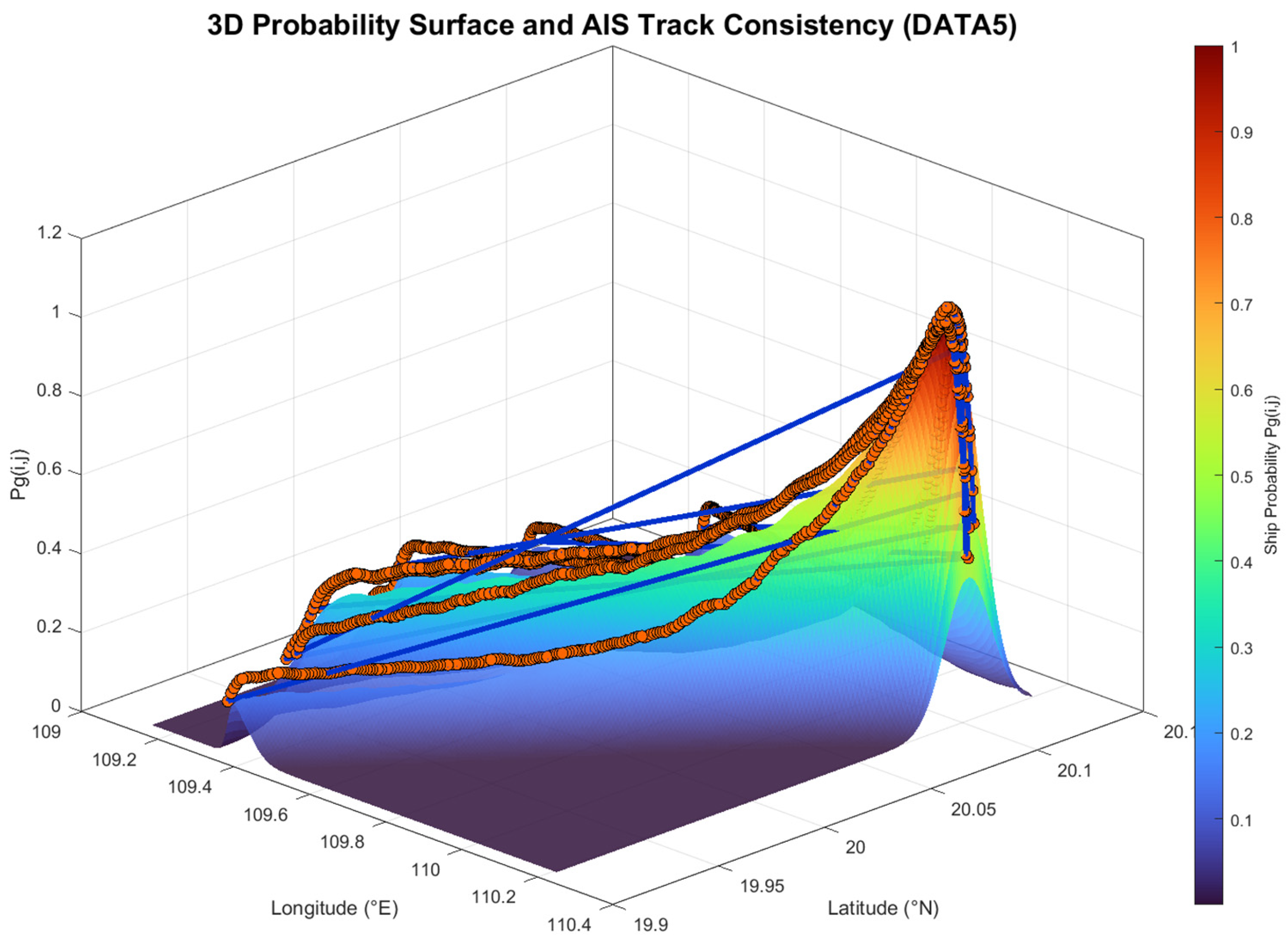
To systematically evaluate the spatial precision of the perception module, this study compares the model-generated 3D ship probability grids ($P_g$) with actual AIS trajectory data. As visually validated in Figure 4, the authentic AIS trajectories (blue lines) consistently traverse the high-probability ridges (red/yellow regions) of the generated 3D probability surface. Quantitative assessment indicates that the model captures the vessel distribution within the main channel. Specifically, in straight-line navigation segments, the trajectory consistency remains stable. Although minor spatial offsets occur during turning maneuvers or low-speed navigation, the overall deviation remains bounded within the scale of a ship’s beam. This confirms that the model translates 2D visual features into robust BEV spatial data, delivering reliable coordinate inputs for the subsequent navigability evaluation without generating physically impossible trajectory drifts.

Figure 4 illustrates the 3D spatial consistency between the model-generated ship probability grids and the actual AIS trajectories. By comparing the 3D probability surface and the actual trajectories in the figure, the precision of the model in reflecting vessel positions and movement trajectories can be clearly observed. Within the main channel region, the high degree of overlap between the model-generated probability grids and the authentic vessel trajectories indicates that the model can capture the probability distribution of vessels at specific locations and map out their movement paths.

Furthermore, the integration of colored contour lines and vessel trajectories in the figure further substantiates the model’s trajectory mapping capability under low-visibility conditions. The movement trajectories of the vessels are represented by blue lines, while the probability surface reflects the probability intensity of vessels at various locations, with red and green regions indicating higher probabilities of vessel passage. This spatial consistency demonstrates that the model can predict vessel positions in complex meteorological environments, delivering robust data support for subsequent navigational decision-making and path planning. In summary, the generated probability grids exhibit robust spatial consistency with actual vessel paths. This confirms that the model provides reliable spatial data to support route monitoring and traffic decision-making under low-visibility conditions.

In practical waterway management, navigational safety is influenced by a multitude of factors, particularly low-visibility foggy weather, which imposes more rigorous demands on the navigability evaluation of the channels. To address this, this study proposes a UAV-based perception method for main navigational routes under fog conditions, utilizing the Sailability Score generated by the model to assist in determining waterway navigability.

4.3. Comparative Analysis Between Sailability Score and VTS Traffic Restriction Windows

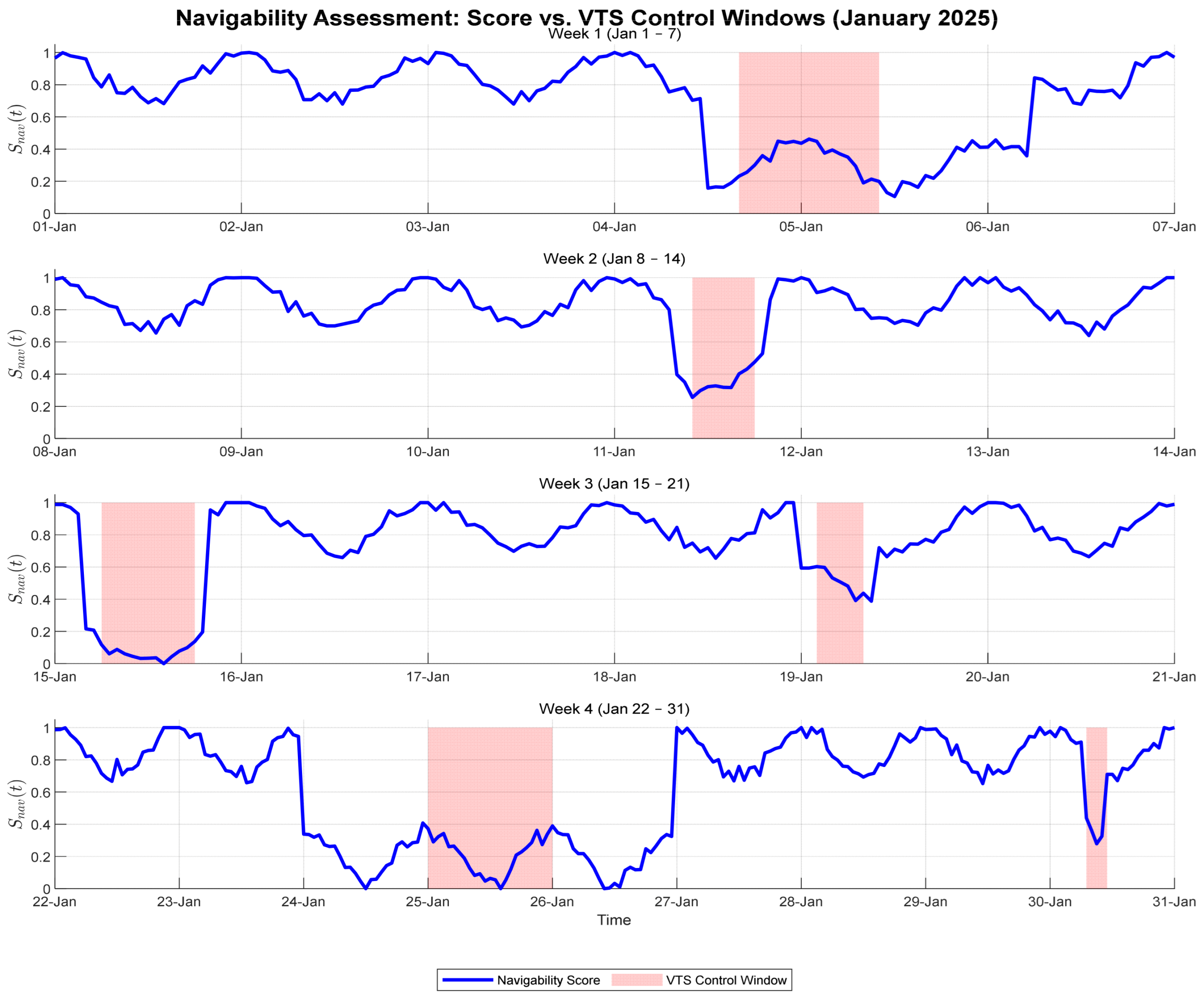
To validate the proposed method in realistic scenarios, a one-month simulated observation experiment was conducted using historical data from 1 January to 31 January 2025. This winter-to-spring transition period features diverse meteorological conditions, including clear weather, sudden advection fog, and prolonged dense fog. The dynamic nature of this dataset provides a representative basis for testing the model’s adaptive capacity across varying visibility levels. Over the course of the 744 h evaluation period, the system operated under a dynamic, event-triggered monitoring strategy rather than uninterrupted 24/7 flight. The simulated UAV swarm was virtually deployed on-demand primarily during high-incidence fog windows (e.g., 05:00–08:00 and 16:00–19:00, as defined in Section Simulation Tasks and Data Collection Workflow). To overcome the approximately 20 min single-flight battery limitation in the simulation environment, the virtual swarm was modeled to adopt a multi-sortie relay rotation strategy (i.e., synchronized take-off and landing cycles among redundant UAV units) to maintain persistent visual coverage during these critical fog events. During clear-weather intervals, the system’s continuous baseline was sustained by uninterrupted shore-based meteorological and AIS data. Following processing via luminance normalization and dehazing enhancement algorithms during the active UAV operational windows, the system calculated in real-time the quantitative metric reflecting the navigability potential of the channel—the Sailability Score $S_{\mathrm{nav}}(t)$. To evaluate the accuracy and reliability of this score, the time-series data output by the model were precisely temporally aligned with the concurrent actual Vessel Traffic Service (VTS) traffic control records of the port. Through this long-term comparative analysis between the “model-calculated values” and the “real-world execution standards,” the objective is to evaluate whether the navigability metrics generated by the model possess practical value across statistical patterns and extreme cases. The specific comparative analysis results are illustrated in Figure 5.

Figure 5 illustrates in detail the time-series comparison results between the model-generated Sailability Score and the actual VTS traffic restriction windows for the entire month of January 2025. In this figure, the blue curve represents the score calculated by the model based on real-time environmental perception, while the red shaded areas indicate the traffic restriction time windows implemented by the VTS center based on real-time meteorological and navigational safety considerations. Analysis of the full-month data indicates that the model’s score curve synchronizes with actual VTS control measures. During clear periods, the score remains between 0.8 and 1.0, reflecting normal navigational conditions. Conversely, upon encountering adverse weather, the score curve exhibits a rapid decline prior to or synchronously with the VTS restriction windows, and the magnitude of the decline is positively correlated with the severity of the weather.

Particularly noteworthy is the data performance during Week 4 (22–31 January), which provides clear evidence for the model’s effectiveness. As illustrated in the figure, between 24 January and 27 January, the port waters experienced a prolonged period of severe dense fog, prompting the VTS to implement continuous channel closures spanning nearly three days. During this period, the model-generated Sailability Score $S_{\mathrm{nav}}(t)$ did not exhibit oscillations or misjudgments; instead, it stably maintained a low value close to 0, forming a broad “U-shaped” trough. This aligns with the long-duration traffic restriction windows, reflecting the sustained loss of channel navigability during this period. In contrast, during the short-term episodic patchy fog events in Week 2 (11 January) and Week 3 (15 January), the model score similarly exhibited rapid “V-shaped” downward responses, aligning with the short-term VTS control windows on the timeline. This correspondence demonstrates the model’s stability under both instantaneous visibility fluctuations and prolonged extreme weather conditions. The analysis results indicate that when $S_{\mathrm{nav}}(t)$ drops to a specific threshold, it accurately predicts the necessity of channel closure controls in actual shipping operations, whereas the upward trend of the score provides a precise reference for the recovery of navigational conditions and the timing of reopening. In summary, the Sailability Score generated by this model can translate subjective visual visibility into objective quantitative data, providing real-time decision-making support for VTS operators in determining when to execute channel closures or reopen navigation under complex weather conditions.

4.4. Quantitative Results of Overall Performance

Building upon the preceding temporal and spatial consistency evaluations, this section quantitatively summarizes the overall performance of the proposed method. To ensure scientific rigor and address the distinct physical characteristics of different modules, the comparative experiment design is explicitly decoupled into three tasks, each configured with a specific benchmark setting:

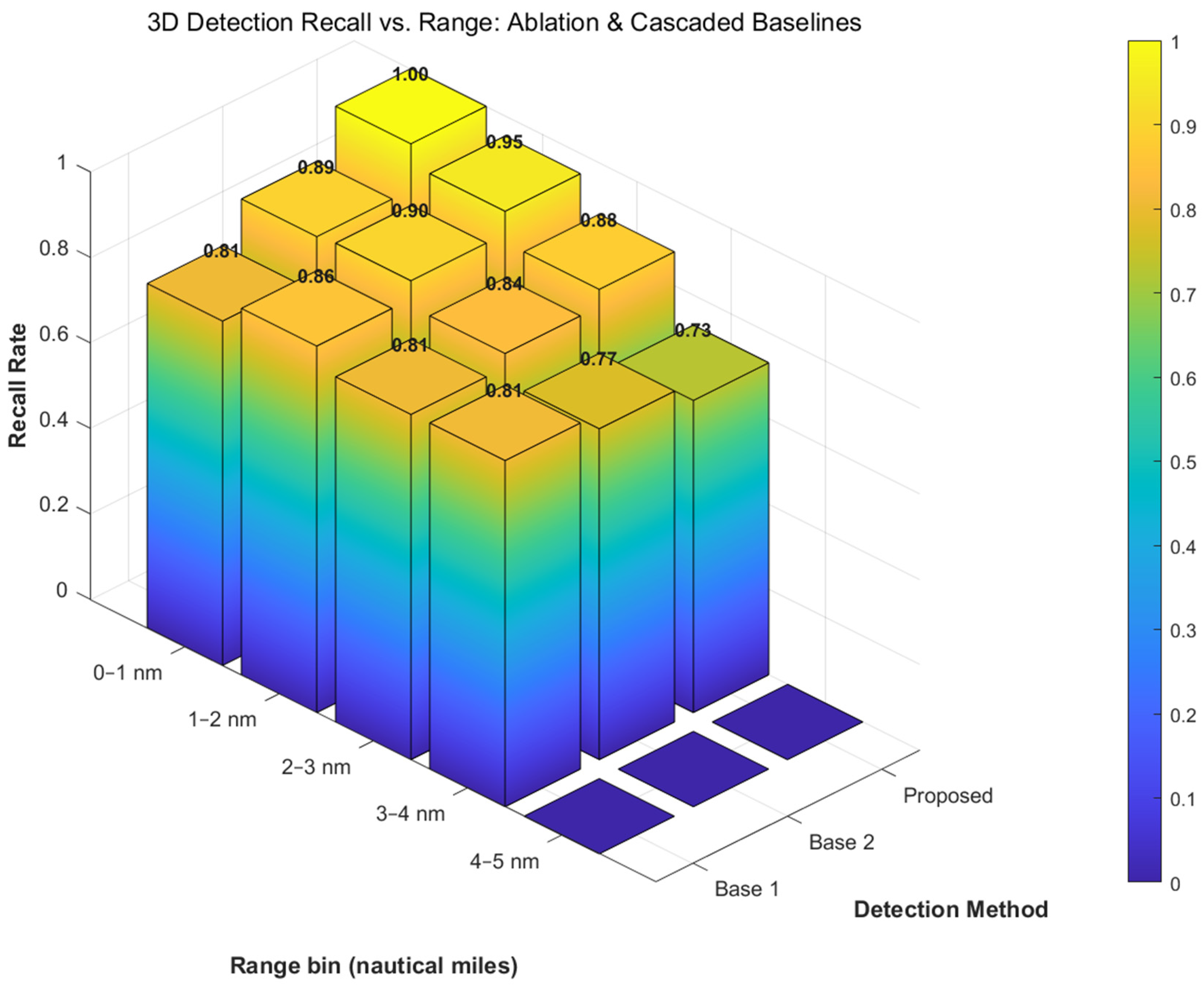
(1) Target Detection Benchmarks: To rigorously evaluate the proposed coupled architecture, we establish two baselines. Baseline 1 (Raw Detection) utilizes the base YOLOv8 network directly on raw foggy images to serve as a pure ablation reference. Baseline 2 (Cascaded Pipeline) represents a contemporary multimodal approach where images are first enhanced by a standard physical dehazing algorithm before being fed into the detector. Comparing our method against Baseline 2 explicitly tests the performance of our physically consistent joint optimization over traditional sequential processing.

(2) Visibility Estimation Benchmark: To evaluate environmental parameter inversion, the benchmark employs a traditional Kriging interpolation scheme relying solely on single-station shore-based observation data. It is crucial to note that this baseline represents the de facto operational standard currently deployed by maritime administrations (e.g., Qiongzhou Strait VTS center). Therefore, this comparison fundamentally evaluates operational effectiveness—demonstrating the transition from traditional 1D point-sensing to the proposed 3D UAV-BEV continuous field.

(3) Decision Support Benchmark: For evaluating navigability recommendations, the benchmark utilizes a rigid thresholding logic based on single-point observations, while historical actual Vessel Traffic Service (VTS) control records serve as the definitive “Ground Truth.”

Based on this comparative framework, the simulation results are consolidated from the dimensions of detection recall, visibility error, decision consistency, and time-window extension.

4.4.1. Long-Distance Small Target Detection Performance

To verify the performance boundaries of the proposed method under extreme perception conditions, this study focuses its evaluation on the most challenging “long-distance and low-visibility” scenarios (target distance > 2.5 nm and visibility ≤ 500 m). In such scenarios, the high-frequency features of ship targets are often severely submerged due to the exponentially accumulated effects of atmospheric scattering. In the comparative analysis of this section, the benchmarks are formulated to isolate our algorithmic contribution. While Baseline 1 establishes the lower bound of performance on raw images, Baseline 2 introduces a critical contemporary comparative dimension. Although the cascaded approach of Baseline 2 visually enhances images, it inherently suffers from “cascading errors”—artificial restoration artifacts from the independent dehazing step disrupt the high-frequency features of distant micro-vessels, leading to severe feature submergence. By replacing this sequential decoupling with our fog-domain adaptive enhancement module, our framework mathematically binds the physical scattering parameters with the detection backbone, bypassing these cascading errors entirely.

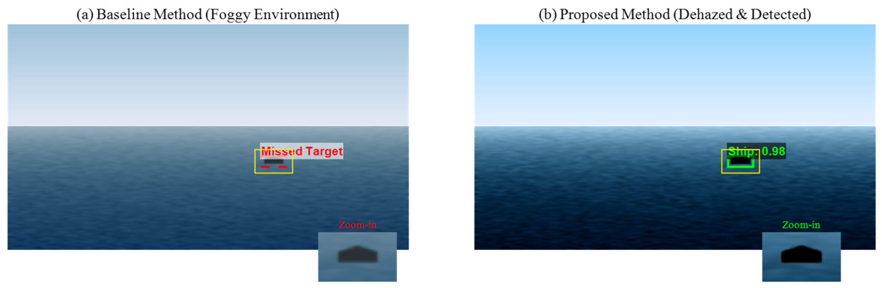
To further elucidate the physical mechanisms underlying the aforementioned 3D statistical features, Figure 6 presents a qualitative visual comparison using a set of typical real-world samples of long-distance fog navigation. The left panel (a) demonstrates that in the raw foggy images, distant vessels near the horizon almost blend into the background wave noise due to exceptionally low contrast. Constrained by insufficient feature extraction capabilities, Baseline 1 results in severe “Missed Target” phenomena. Furthermore, while the cascaded Baseline 2 (evaluated quantitatively in Figure 7) attempts to recover contrast, its decoupled nature introduces artificial artifacts that often mislead bounding box regression. In contrast, by directly coupling the physical prior with the detection backbone, the proposed perception framework (right panel b) exhibits enhanced visual penetrability without introducing cascading errors. The dehazing module suppresses the interference of the atmospheric light veil, enabling the contour edges of the distant vessel to be reconstructed. Consequently, the detection network identifies the target with a confidence score of 0.98. The 3D data in Figure 7 and visual evidence in Figure 6 demonstrate that the proposed joint optimization improves long-distance detection by reconstructing vessel contours otherwise obscured by the atmospheric light veil. This enhancement in perceptual capability bears considerable engineering value: assuming a navigational speed of 15 knots, the 16.2% improvement in the far-field recall rate implies that regulatory systems or autonomous vessels can detect potential collision risks earlier. This secures an additional time window for collision avoidance decision-making—specifically, the Time-to-Collision (TTC)—thereby enhancing the safety resilience of intelligent shipping systems.

4.4.2. Visibility Estimation Precision and Error Analysis

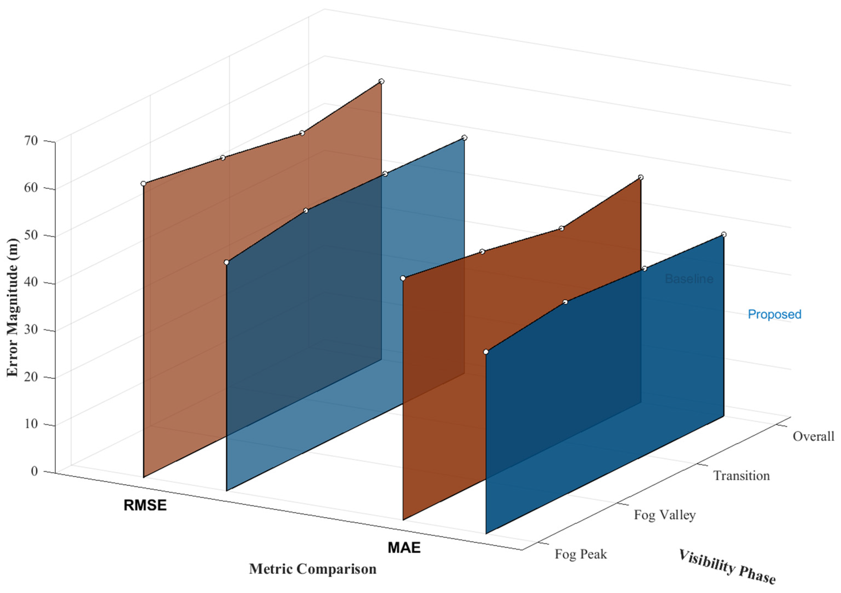
To quantitatively evaluate the precision enhancement of the proposed method, a systematic comparison was conducted between the UAV-based fusion inversion approach (Proposed Method) and the baseline method (Baseline Method). The baseline method employs a traditional Kriging interpolation scheme relying on single-station shore-based observation data. Mean Absolute Error (MAE) and Root Mean Square Error (RMSE) were selected as the primary evaluation metrics, and statistical analyses were, respectively, conducted across the three previously defined visibility phases: the fog peak, fog valley, and transition phases.

Table 4. Statistical error comparison between the baseline and proposed methods across different visibility phases.

Visibility Phase	Method	Mean Absolute Error (MAE) (m)	Root Mean Square Error (RMSE) (m)	Performance Improvement (Based on MAE)
Fog Peak Phase (Visibility < 600 m)	(Baseline)	51.2	62.15	-
	(Proposed)	38.52	48.4	24.80%
Fog Valley Phase (600 m–1000 m)	(Baseline)	48.5	59.3	-
	(Proposed)	40.75	51	16.00%
Transition Phase (>1000 m)	(Baseline)	45.1	56.2	-
	(Proposed)	39.49	50.47	12.40%
Overall Average	(Baseline)	47.6	58.85	-
	(Proposed)	38.41	49.82	19.30%

presents a detailed comparison of the error statistics between the baseline method and the proposed method across various visibility phases. From the perspective of overall performance, the proposed UAV-based fusion inversion architecture exhibits improved precision. It reduces the full-period Mean Absolute Error (MAE) from 47.60 m in the baseline method to 38.41 m, corresponding to a relative precision improvement of 19.3%. Further phase-specific analysis reveals the robustness of this method in extreme environments. During the fog peak phase, which entails the highest navigational risk (visibility < 600 m), the severe spatial heterogeneity of sea fog causes the Root Mean Square Error (RMSE) of the traditional baseline method to surge to 62.15 m. Conversely, by incorporating physical dehazing and feature calibration from an aerial perspective, the proposed method constrains the RMSE to 48.40 m, achieving a maximum MAE improvement of 24.8% across all phases. As visibility gradually improves, transitioning into the fog valley phase (600–1000 m) and the transition phase (>1000 m), the performance of the baseline method exhibits some recovery. Nevertheless, the proposed method sustains a stable leading advantage, yielding precision improvements of 16.0% and 12.4%, respectively. This trend of error reduction demonstrates that, compared to traditional approaches relying on single-point interpolation, visibility field modeling integrated with UAV perception data can more accurately characterize the authentic navigability conditions in complex fog navigation environments.

Delving deeper from an engineering perspective, the distinct stratified gap between the blue error band (proposed method) and the orange error band (baseline method) in Figure 8 clearly highlights the intrinsic limitations of traditional single-point observations in coping with the spatial heterogeneity of sea fog. The significant error fluctuations exhibited by the baseline method during the fog peak and fog valley phases primarily stem from the inability of shore-based stations to accurately perceive the dynamics of localized patchy fog in the central channel or distant waters. Such a representational bias—substituting the entire region with a single point—makes the Vessel Traffic Service (VTS) system highly susceptible to a decision-making dilemma: erroneously mandating channel closures due to dense coastal fog, or riskily reopening navigation based merely on coastal fog dissipation. In contrast, by bridging the spatial information blind spots in offshore waters, the proposed UAV-based fusion inversion architecture compresses the overall deviation of visibility estimation by nearly 20%. This physical-level precision gain represents far more than a mere optimization of statistical figures; it signifies that the perception system can filter out localized meteorological noise. Consequently, it provides reliable environmental parameter inputs for the subsequently constructed Sailability Score model, ensuring that final navigational decisions are grounded in the observed environmental state of the channel, rather than extrapolations derived from discrete station data.

4.4.3. Decision Consistency Analysis Between Sailability Score and Control Records

To verify the engineering applicability of the proposed Sailability Score in practical maritime regulatory operations, and to examine the degree of concordance between the algorithm’s decision-making logic and human expert experience, this section utilizes historical actual Vessel Traffic Service (VTS) control records as the “Ground Truth.” By mapping the quantitative scores output by the model into binary control recommendations, a 3D Decision Consistency Landscape is constructed (as illustrated in Figure 9). Utilizing the elevation and volume of the topographic peaks, this visual model intuitively characterizes the temporal aggregation density and distribution patterns under various decision combinations.

This figure illustrates the matching distribution between the model’s Sailability Score and the actual VTS control records. The twin peaks of True Negative (TN) and True Positive (TP) along the main diagonal constitute the primary body of high consistency (82.1%). Meanwhile, the asymmetric topography in the off-diagonal regions—where the “false alarm peak” is significantly higher than the “missed detection valley”—reveals the model’s safety-conservative preference of “better a false alarm than a missed detection.”

The 3D landscape exhibits two main peaks along the diagonal, corresponding to True Negatives (TN, 52.8%) and True Positives (TP, 29.3%). These peaks collectively account for 82.1% of the samples, indicating a high quantitative alignment between the model’s outputs and actual VTS control rules. that is, the algorithm can distinguish between “safe navigation periods” and “high-risk restriction periods” just consistent with expert decisions.

Further examining the “saddle” morphology in the non-main-peak regions, the landscape exhibits pronounced Asymmetry characteristics: the region representing “Conservative False Positives (FP)” bulges to form a clearly visible secondary hill (11.6%), whose elevation is significantly higher than the valley region representing “False Negative Risks (FN)” (6.3%). This topographic elevation disparity of a “high false alarm peak and low missed detection valley” concretizes the model’s Safety Conservativeness from a topological perspective. This implies that in the marginal zones of visibility fluctuations, the model tends to “dissipate” prediction errors towards the safe side (i.e., preferring to erroneously advise a restriction) rather than the risk side. From the perspective of traffic engineering practice, this characteristic ensures that the auxiliary system can proactively tighten safety boundaries when confronting environmental uncertainties, thereby providing reliable support and a safety redundancy buffer for maritime regulation.

From the perspective of maritime operational safety and economic efficiency, the consequences of these decision discrepancies are fundamentally asymmetric. False Negative (FN) errors, characterized as “missed warnings,” represent the most critical risk, as they might lead vessels to enter hazardous low-visibility areas, directly increasing the probability of collisions or groundings. Given that a single maritime accident in the Qiongzhou Strait could result in catastrophic environmental damage and loss of life, the model’s design intentionally prioritizes safety (reflected by $\eta >1$) to eliminate these high-risk FN scenarios. Conversely, False Positive (FP) errors (false alarms) primarily lead to “over-caution,” resulting in unnecessary vessel queuing at anchorage, increased fuel consumption, and logistical delays. While these impose economic costs on shipping companies, they serve as a necessary trade-off for maintaining a zero-accident safety baseline in complex fog environments.

4.4.4. Navigable Time-Window Extension Analysis Under Dynamic Fog Conditions

Beyond static decision consistency, in marginal scenarios where visibility fluctuates frequently near the critical threshold ($V_t$ ≈ 500 m), the temporal stability of the perception system directly dictates the Effective Navigable Efficiency of the channel. Traditional single-point observation methods often employ rigid thresholding, which is highly susceptible to localized patchy fog interference. This susceptibility leads to frequent switching between “open” and “restricted” navigational commands—a phenomenon known as the “Ping-pong Effect”—which results in a substantial amount of fragmented downtime. To quantify the engineering value of the proposed method in enhancing navigational efficiency, this section selects a typical 5 h dataset of critical fog fluctuations to compare the temporal distribution of control states between the baseline method and the proposed method (as illustrated in Figure 10).

First, focus on the evolutionary characteristics of the physical environment as illustrated in Figure 10a. This sub-figure simulates a highly challenging “marginal weather” scenario in maritime regulation. The blue curve in the figure depicts the visibility readings exhibiting pronounced oscillatory behavior around the control threshold $V_t$ = $V_0$ (500 m) within a 5 h observation window. This high-frequency fluctuation is not merely measurement noise; rather, it provides an accurate representation of the unstable physical processes during the generation and dissipation phases of patchy fog. In such an environment, visibility values frequently traverse between the judgment boundaries of “navigable” and “restricted,” posing a significant decision-making challenge for traditional regulatory modes that rely solely on instantaneous thresholding.

Based on the aforementioned environmental inputs, Figure 10b further illustrates the temporal response disparities between the two distinct decision-making logics. Due to the lack of a temporal filtering mechanism, the baseline method (blue shaded area) mechanically couples with every numerical fluctuation shown in Figure 10a. This leads to seven instances of short-term channel closures within a mere 5 h window. Such fragmented control directives cause the channel status to repeatedly oscillate between “OPEN” and “CLOSED,” which increases the risk of uncoordinated vessel maneuvers and traffic flow congestion within port waters.

In contrast, the proposed method (orange curve) utilizes the hysteresis filtering mechanism to smooth out transient fluctuations, maintaining stability in the decision-making commands throughout the period.

4.4.5. Real-Time UAV Feasibility and Latency Analysis

To evaluate the framework’s potential deployability, the end-to-end closed-loop latency was estimated in the simulation. As illustrated in Figure 11, the cumulative system latency is tightly constrained to 190 ms ($f_{sys}\approx 5.2$ FPS), comprising data link transmission (150 ms) and computational processing (40 ms). For a typical vessel navigating at 15 knots, the positional displacement during this sub-second processing window is merely 1.46 m. This physically negligible redundancy confirms that the framework remains highly responsive to dynamic environmental fluctuations under operational maritime conditions.

4.5. Sensitivity and Robustness Analysis

The dynamic feedback and time-window optimization model constructed in this study involves the configuration of several key control variables. To explore the performance boundaries of the proposed perception framework under various configurations and to verify the system’s robustness in engineering applications, this section conducts a sensitivity analysis on two core hyperparameters that dictate decision stringency and temporal stability.

The first is the navigability determination threshold ($S_{thr}$), which corresponds to the defined risk assessment boundary and directly determines the triggering conditions of the binary decision function $\mathbb{I}(S_{nav}\ge S_{thr})$. The second is the temporal smoothing window ($T_{smooth}$), an engineering parameter introduced to solve the integral formula for the navigable time window $T_{\mathrm{nav}}$ defined in Section 2.7 within the discrete time domain. During the actual calculation process, directly integrating the noisy raw score sequence would lead to severe fragmentation in the results of $T_{\mathrm{nav}}$; therefore, $T_{smooth}$ must be introduced for time-domain preprocessing. Through quantitative trade-off experiments, this section determines the optimal values for these two parameters under the constraints of both safety and efficiency.

4.5.1. Impact of Determination Threshold $S_{thr}$ on Decision Consistency

To quantitatively analyze the impact of the navigability determination threshold $S_{thr}$ on the model’s decision-making behavior, Figure 12 illustrates the evolutionary patterns of the decision consistency overlap rate (Z) and the safety preference ratio ($\eta$ = FP/FN) within the interval $S_{thr}$∈[20, 80]. Based on the trend of the consistency index Z shown in the figure, as $S_{thr}$ increases, the accuracy exhibits a typical inverted U-shaped distribution, first rising and then declining, reaching its peak (82.1%) at $S_{thr}$ approx. 45. This indicates that thresholds set either too low or too high will cause the model’s determination logic to deviate from the cognitive benchmarks of human experts. Simultaneously, observing the safety preference ratio $\gamma$ on the right axis, it is evident that this metric increases monotonically with the threshold. Notably, when $S_{thr}$ > 40, $\eta$ remains consistently greater than 1, implying that the system at this point tends to generate “conservative false alarms” rather than “aggressive missed detections.” Considering both high consistency and the necessary safety bottom line, this study ultimately selects in [40, 50] as the optimal confidence interval. Within this range, the model can emulate the decision-making logic of VTS experts while maintaining reasonable safety redundancy.

4.5.2. Impact of Smoothing Window $T_{smooth}$ on Temporal Stability

To quantitatively evaluate the practical impact of the smoothing window $T_{smooth}$ on the overall system performance, two specific evaluation metrics are introduced: Switching Frequency ($F_{sw}$), defined as the number of state transitions per unit time to characterize decision stability; and Response Delay ($D_{res}$), defined as the average lag time required for the model to identify sudden patchy fog to characterize early-warning timeliness. Based on these metrics, Figure 13 clearly illustrates the trade-off relationship established by the window size $T_{smooth}$ between stability and timeliness. Simulation results suggest that as $T_{smooth}$ increases, $F_{sw}$ exhibits a significant exponential decay trend, suggesting that a wider window can enhance the jitter-suppression capability of the integral calculation and filter out high-frequency environmental noise. However, this comes at the cost of a linear upward trend in $D_{res}$, leading to a perception lag regarding sudden fog events. Specifically, when $T_{smooth}$ < 5 min, the integration results are highly unstable and prone to frequent command switching triggered by disturbances. Conversely, when $T_{smooth}$ > 15 min, the average response delay exceeds the safety tolerance limit, which may cause the calculated $T_{\mathrm{nav}}$ to deviate from the actual safety window. Based on the above analysis, this study selects $T_{smooth}$ = 10 as the optimal engineering parameter for solving the optimization objective, which filters out over 95% of unnecessary fluctuations while ensuring a timely response to sudden meteorological events.

Furthermore, the delayed recovery recommendations associated with a larger smoothing window $T_{smooth}$ represent an opportunity cost in navigational efficiency. A lag in reopening the channel after fog dissipation means that vessels remain anchored even when conditions are safe, potentially leading to port congestion. However, in the context of Vessel Traffic Service (VTS) operations, this delay acts as a “safety buffer” to ensure that the meteorological state has stabilized across the entire BEV field, preventing the “ping-pong effect” of frequent opening and closing which can confuse navigators and induce maneuvering risks.

5. Conclusions and Future Work

5.1. Summary

This study proposes a UAV-based collaborative perception and sailability assessment framework, integrating physical models with marine engineering to address maritime traffic regulation under dynamic sea fog. Based on multi-source data validation in the Qiongzhou Strait, the primary conclusions are quantitatively summarized as follows:

(1)

High-Precision Visibility Inversion:

By projecting physical-prior features into a continuous Bird’s-Eye View (BEV) space, the model mitigates the spatial representativeness errors inherent in single-station sensors. Quantitative simulation comparisons suggest that the Mean Absolute Error (MAE) of visibility estimation is reduced by 19.3%.

(2)

Robust Perception via Physically Consistent Joint Optimization:

Moving beyond a trivial system-level assembly of existing algorithms, the framework establishes a deeply coupled architecture where atmospheric scattering parameters simultaneously constrain both visual restoration and target recognition. By utilizing the inverted transmittance field as a latent physical anchor to dynamically re-weight detection feature channels via a fog-domain adaptive mechanism (${\alpha }_t$), the system overcomes the “cascading errors” inherent in traditional decoupled pipelines. Coupled with the UAV’s unique Bird’s-Eye View (BEV), this physically grounded integration prevents performance collapse in non-homogeneous patchy fog. Under marginal operating conditions (visibility ≤ 500 m), the detection recall rate for long-distance micro-vessels is improved by 16.2% compared to traditional baseline models, indicating that the integration of physical priors with deep learning architectures facilitates the transition from local sensing to global spatial risk quantification.

(3)

Synergistic Decision Optimization:

The proposed Sailability Score model achieves an 82.1% operational consistency with historical VTS expert decisions. Benefiting from a temporal integration optimization window ($\Delta t=10$ min), the system filters high-frequency environmental noise, extending the navigable time window by 12.4% while maintaining a conservative safety baseline ($\gamma >1$).

5.2. Limitations and Future Work

While the proposed integrated perception framework demonstrates robust performance, certain hardware and scenario constraints remain. Future research will focus on the following three dimensions:

(1)

All-Weather Multi-Modal Fusion:

Current visual enhancement relies on the visible light spectrum (DCP). Future work will incorporate infrared thermal imaging at the feature level to compensate for illumination dependencies at night and in dense fog, facilitating the transition from “daytime fog navigation” to “all-weather, full-time” regulation.

(2)

Model Lightweighting for Edge Computing

Given the strict computational and energy constraints of UAV-onboard systems, future efforts will prioritize lightweighting strategies (e.g., model pruning, knowledge distillation) to reduce algorithmic latency, fulfilling the rigorous demands of instantaneous edge-side decision-making.

(3)

Active UAV Guidance and Perceptual-Control Coupling

From a guidance and control perspective, the current framework primarily serves as a high-level perception and decision-support system for VTS operators, rather than a genuine closed-loop physical controller. It currently lacks specific UAV guidance laws, trajectory replanning logic, and aerodynamic stability analyses. Future research will focus on deep Perceptual-Control Coupling. Utilizing the BEV visibility and ship probability grids generated in this study, we aim to develop robust, closed-loop control algorithms (e.g., Nonlinear Model Predictive Control) to dynamically replan UAV flight trajectories and collision avoidance strategies in real-time, thereby propelling the system from passive auxiliary perception to active, autonomous safe cruising.

(4)

Real-World Hardware Validation

As the current framework has been evaluated primarily through data-driven simulations, future work must prioritize real-world hardware deployments. Actual physical flight tests in fog-prone waterways are essential to validate the framework’s robustness against unmodeled environmental disturbances (e.g., severe wind shear, complex sea clutter) and to verify its reliability under true edge-computing hardware constraints.

References

1. Song, S.; Chen, Y.; Chen, X.; Chen, C.; Li, K.; Tung, K.; Shao, Q.; Liu, Y.; Wang, X.; Yi, L.; et al. Adapting to a foggy future along trans-arctic shipping routes. Geophys. Res. Lett. 2023, 50, e2022GL102395. [Google Scholar] [CrossRef]
2. Ding, C.; Li, J.; Zhong, W.; Li, F. Observation and simulation of a heavy fog event in Qiongzhou Strait. J. Atmos. Sol. -Terr. Phys. 2022, 240, 105958. [Google Scholar] [CrossRef]
3. Kim, Y.; Ryu, H.S.; Hong, S. Data-to-data translation-based nowcasting of specific sea fog using geostationary weather satellite observation. Atmos. Res. 2023, 290, 106792. [Google Scholar] [CrossRef]
4. Yi, L.; Li, M.; Liu, S.; Shi, X.; Li, K.F.; Bendix, J. Detection of dawn sea fog/low stratus using geostationary satellite imagery. Remote Sens. Environ. 2023, 294, 766–771. [Google Scholar] [CrossRef]
5. Liu, J.; Yu, J.; Lin, C.; He, M.; Liu, H.; Wang, W.; Min, M. Near-real-time atmospheric and oceanic science products of Himawari-8 and Himawari-9 geostationary satellites over the South China Sea. Earth Syst. Sci. Data 2024, 16, 4949–4969. [Google Scholar] [CrossRef]
6. Narasimhan, S.G.; Nayar, S.K. Vision and the atmosphere. Int. J. Comput. Vis. 2002, 48, 233–254. [Google Scholar] [CrossRef]
7. Fattal, R. Dehazing using color-lines. ACM Trans. Graph. 2014, 34, 1–14. [Google Scholar] [CrossRef]
8. Yang, K.; Xiang, W.; Chen, Z.; Zhang, J.; Liu, Y. A review on infrared and visible image fusion algorithms based on neural networks. J. Vis. Commun. Image Represent. 2024, 101, 104179. [Google Scholar] [CrossRef]
9. Zhu, H.; Cheng, Y.; Peng, X.; Zhou, J.T.; Kang, Z.; Lu, S.; Fang, Z.; Li, L.; Lim, J.-H. Single-image dehazing via compositional adversarial network. IEEE Trans. Cybern. 2019, 51, 829–838. [Google Scholar] [CrossRef]
10. He, K.; Sun, J.; Tang, X. Single image haze removal using dark channel prior. IEEE Trans. Pattern Anal. Mach. Intell. 2010, 33, 2341–2353. [Google Scholar] [CrossRef]
11. Zhu, Q.; Mai, J.; Shao, L. A fast single image haze removal algorithm using color attenuation prior. IEEE Trans. Image Process. 2015, 24, 3522–3533. [Google Scholar] [CrossRef]
12. Fattal, R. Single image dehazing. ACM Trans. Graph. 2008, 27, 1–9. [Google Scholar] [CrossRef]
13. Fu, H.; Ling, Z.; Sun, G.; Ren, J.; Zhang, A.; Zhang, L.; Jia, X. HyperDehazing: A hyperspectral image dehazing benchmark dataset and a deep learning model for haze removal. ISPRS J. Photogramm. Remote Sens. 2024, 218, 663–677. [Google Scholar] [CrossRef]
14. Ma, X.; Wang, Q.; Tong, X.; Atkinson, P.M. A deep learning model for incorporating temporal information in haze removal. Remote Sens. Environ. 2022, 274, 113012. [Google Scholar] [CrossRef]
15. Yang, G.; Li, J.; Lei, H.; Gao, X. A multi-scale information integration framework for infrared and visible image fusion. Neurocomputing 2024, 600, 128116. [Google Scholar] [CrossRef]
16. Xie, Y.; Nanlal, C.; Liu, Y. Reliable LiDAR-based ship detection and tracking for Autonomous Surface Vehicles in busy maritime environments. Ocean Eng. 2024, 312, 119288. [Google Scholar] [CrossRef]
17. Qu, J.; Liu, R.W.; Guo, Y.; Lu, Y.; Su, J.; Li, P. Improving maritime traffic surveillance in inland waterways using the robust fusion of AIS and visual data. Ocean Eng. 2023, 275, 114198. [Google Scholar] [CrossRef]
18. Chen, X.; Chen, W.; Wu, B.; Wu, H.; Xian, J. Ship visual trajectory exploitation via an ensemble instance segmentation framework. Ocean Eng. 2024, 313, 119368. [Google Scholar] [CrossRef]
19. Tu, E.; Zhang, G.; Rachmawati, L.; Rajabally, E.; Huang, G.-B. Exploiting AIS data for intelligent maritime navigation: A comprehensive survey from data to methodology. IEEE Trans. Intell. Transp. Syst. 2017, 19, 1559–1582. [Google Scholar] [CrossRef]
20. Zhao, C.; Liu, R.W.; Qu, J.; Gao, R. Deep learning-based object detection in maritime unmanned aerial vehicle imagery: Review and experimental comparisons. Eng. Appl. Artif. Intell. 2024, 128, 107513. [Google Scholar] [CrossRef]
21. Yang, X.; Huo, H.; Li, J.; Li, C.; Liu, Z.; Chen, X. DSG-fusion: Infrared and visible image fusion via generative adversarial networks and guided filter. Expert Syst. Appl. 2022, 200, 116905. [Google Scholar] [CrossRef]
22. Pande, S.; Banerjee, B. Self-supervision assisted multimodal remote sensing image classification with coupled self-looping convolution networks. Neural Netw. 2023, 164, 1–20. [Google Scholar] [CrossRef]
23. Brandt, P.; Munim, Z.H.; Chaal, M.; Kang, H.-S. Maritime accident risk prediction integrating weather data using machine learning. Transp. Res. Part D: Transp. Environ. 2024, 136, 104388. [Google Scholar] [CrossRef]
24. Zhang, M.; Taimuri, G.; Zhang, J.; Zhang, D.; Yan, X.; Kujala, P.; Hirdaris, S. Systems driven intelligent decision support methods for ship collision and grounding prevention: Present status, possible solutions, and challenges. Reliab. Eng. Syst. Saf. 2025, 253, 110489. [Google Scholar] [CrossRef]
25. Sánchez-González, A.; Rodrigues-Tomé, S.R.; Cardoso-Mestre, D.; García-Maza, J.A. Reliability of maritime collision avoidance systems algorithms in the implementation of COLREGs. Reliab. Eng. Syst. Saf. 2025, 267, 111840. [Google Scholar] [CrossRef]
26. Qiu, S.; Wang, S.; Chen, X.; Qian, F.; Xiao, Y. Ship shape reconstruction for three-dimensional situational awareness of smart ships based on neural radiation field. Eng. Appl. Artif. Intell. 2024, 136, 108858. [Google Scholar] [CrossRef]
27. Dong, A.; Wang, L.; Liu, J.; Lv, G.; Zhao, G.; Cheng, J. MFIFusion: An infrared and visible image enhanced fusion network based on multi-level feature injection. Pattern Recognit. 2024, 152, 110445. [Google Scholar] [CrossRef]
28. Yi, S.; Guo, S.; Chen, M.; Wang, J.; Jia, Y. UIRGBfuse: Revisiting infrared and visible image fusion from the unified fusion of infrared channel with R, G, and B channels. Infrared Phys. Technol. 2024, 143, 105626. [Google Scholar] [CrossRef]
29. Wang, Z.; Yang, F.; Wang, J.; Xu, J.; Yang, F.; Ji, L. A dual-path residual attention fusion network for infrared and visible images. Optik 2023, 290, 171251. [Google Scholar] [CrossRef]
30. Liu, R.; Liu, Y.; Wang, H.; Du, S. WaveFusionNet: Infrared and visible image fusion based on multi-scale feature encoder–decoder and discrete wavelet decomposition. Opt. Commun. 2024, 573, 131024. [Google Scholar] [CrossRef]
31. Sakaridis, C.; Dai, D.; Hecker, S.; Van Gool, L. Curriculum model adaptation with synthetic and real data for semantic foggy scene understanding. Int. J. Comput. Vis. 2020, 128, 1182–1204. [Google Scholar]
32. Nuss, D.; Reuter, S.; Thom, M.; Yuan, T.; Krehl, G.; Maile, M.; Gern, A.; Dietmayer, K. A random finite set approach for dynamic occupancy grid maps with real-time application. Int. J. Robot. Res. 2018, 37, 841–866. [Google Scholar] [CrossRef]
33. Zhao, J.; Shi, J.; Zhuo, L. BEV perception for autonomous driving: State of the art and future perspectives. Expert Syst. Appl. 2024, 258, 125103. [Google Scholar] [CrossRef]
34. Zhang, M.; Montewka, J.; Manderbacka, T.; Kujala, P.; Hirdaris, S. A big data analytics method for the evaluation of ship-ship collision risk reflecting hydrometeorological conditions. Reliab. Eng. Syst. Saf. 2021, 213, 107674. [Google Scholar] [CrossRef]
35. Du, L.; Goerlandt, F.; Kujala, P. Review and analysis of methods for assessing maritime waterway risk based on non-accident critical events detected from AIS data. Reliab. Eng. Syst. Saf. 2020, 200, 106933. [Google Scholar] [CrossRef]
36. NGA.STND.0036_1.0.0_WGS84; Department of Defense World Geodetic System 1984, Its Definition and Relationships with Local Geodetic Systems. National Geospatial-Intelligence Agency: Springfield, VA, USA, 2014.
37. ISO 21384-3:2019; Unmanned Aircraft Systems—Part 3: Operational Procedures. International Organization for Standardization (ISO): Geneva, Switzerland, 2019.
Figure 1. System architecture of UAV-based perception for mainway fog navigation.
Drones 10 00367 g001
Figure 2. Illustration of the experimental area and UAV flight trajectories.
Drones 10 00367 g002
Figure 3. Visibility fluctuations and model prediction error analysis in the Qiongzhou Strait (January 2025).
Drones 10 00367 g003
Figure 4. 3D trajectory consistency analysis based on vessel probability grids.
Drones 10 00367 g004
Figure 5. Comparison between the model-generated Sailability Score and VTS traffic restriction windows.
Drones 10 00367 g005
Figure 6. Qualitative visual comparison of small target detection performance under dense fog conditions.
Drones 10 00367 g006
Figure 7. Detection recall vs. distance. Base 1: raw generic detector; Base 2: cascaded pipeline; Proposed: physically consistent joint optimization.
Drones 10 00367 g007
Figure 8. 3D topographical distribution of visibility estimation errors across different fog phases.
Drones 10 00367 g008
Figure 9. 3D topographical landscape of decision consistency between model outputs and VTS records.
Drones 10 00367 g009
Figure 10. 3D analysis of visibility fluctuations and navigational time-window extension under dynamic marginal weather.
Drones 10 00367 g010
Figure 11. End-to-end system latency breakdown and real-time feasibility validation.
Drones 10 00367 g011
Figure 12. Sensitivity analysis of the navigability determination threshold.
Drones 10 00367 g012
Figure 13. Impact analysis of the temporal smoothing window T s m o o t h on system performance.
Drones 10 00367 g013