Article

Aerostructural Optimization of a Composite Low Reynolds Wing Using Surrogate Modeling Techniques

by
Eleftherios Nikolaou
1,*,
Spyridon Kilimtzidis
1,*,
Panagiota Kelverkloglou
1,†,
Vaios Lappas
2,† and
Vassilis Kostopoulos
1,†
1
Applied Mechanics Laboratory, Mechanical Engineering and Aeronautics Department, University of Patras, Rio Campus, 26500 Patras, Greece
2
Department of Aerospace Science and Technology, National and Kapodistrian University of Athens, 10679 Athens, Greece
*
Authors to whom correspondence should be addressed.
These authors contributed equally to this work.
Drones 2026, 10(5), 352; https://doi.org/10.3390/drones10050352
Submission received: 22 March 2026 / Revised: 4 May 2026 / Accepted: 5 May 2026 / Published: 7 May 2026
(This article belongs to the Special Issue Dynamics Modeling and Conceptual Design of UAVs—2nd Edition)

Highlights

What are the main findings?
  • A CFD-FEM-based aerostructural optimization framework using Kriging-based SBO achieves consistent convergence to feasible, high-performance UAV wing designs.
  • Aerodynamic variables (mainly aspect ratio and twist) dominate range performance, while structural variables (especially skin thickness) govern constraint satisfaction and define the feasible design space.
What are the implications of the main findings?
  • Early-stage UAV wing design can effectively incorporate high-fidelity aerostructural coupling with reduced computational cost through surrogate-based optimization.
  • Optimal designs emerge from balancing aerodynamic performance and structural constraints, highlighting the necessity of multidisciplinary optimization for realistic and efficient configurations.

Abstract

This study presents an aerostructural optimization framework for the preliminary design of a low-Reynolds-number composite UAV wing, aiming to simultaneously enhance aerodynamic efficiency and structural performance. While previous work has primarily addressed aerodynamic optimization in isolation, the present approach integrates Computational Fluid Dynamics (CFD) and Finite Element Method (FEM) analyses within a surrogate-based optimization (SBO) framework. The design space includes both aerodynamic parameters—aspect ratio, taper ratio, sweep angle, and twist—and structural variables related to the internal wing layout and component thicknesses. To reduce the computational cost associated with high-fidelity simulations, Kriging surrogate models are employed in conjunction with an Expected Improvement (EI) infill strategy, enabling efficient exploration of the coupled design space. The framework is evaluated through multiple independent optimization runs using different initial sampling strategies, demonstrating consistent convergence toward feasible high-performance designs. The surrogate models exhibit strong predictive capability, as confirmed by Root Mean Square Error (RMSE) and Leave-One-Out (LOO) cross-validation metrics. The results indicate that aerodynamic variables, particularly aspect ratio and twist, are the primary drivers of range performance. However, structural variables—most notably skin thickness—strongly influence constraint satisfaction, especially with respect to buckling and strength requirements, and therefore play a key role in defining the feasible design space. The optimal configuration achieves a maximum range of approximately 203 km while satisfying all strength, stiffness, and aerodynamic constraints. Overall, the proposed methodology provides an efficient and robust tool for the early-stage aerostructural design of low-Reynolds-number UAV wings.

1. Introduction

The wing plays a fundamental role in determining the overall performance of an aircraft, as aerodynamic efficiency and structural weight are strongly coupled through the wing geometry and internal layout. Key performance metrics, such as the lift-to-drag ratio ( L / D ) and take-off weight, are directly influenced by aerodynamic characteristics and structural efficiency. Consequently, careful wing design and optimization are essential to achieving an effective and well-balanced aircraft configuration. During the preliminary design phase, the aerodynamic efficiency of the wing largely dictates the expected performance of the complete aircraft, making early-stage wing optimization a critical step in guiding subsequent design decisions.
Aircraft designers therefore aim to identify optimal configurations from both aerodynamic and structural perspectives. Aerodynamic performance is influenced by parameters such as aspect ratio ( A R ), taper ratio ( λ ), sweep angle ( Λ ), and twist ( ϵ ), while the structural configuration is governed by material selection, internal layout (e.g., ribs and spars), and the thickness of structural components, all of which significantly affect the final weight and structural performance.
Over the past decades, numerous studies have investigated various aspects of wing optimization. From an aerodynamic perspective, Lyu et al. [1] performed aerodynamic shape optimization of a benchmark wing using a gradient-based algorithm coupled with Reynolds-Averaged Navier–Stokes (RANS) equations and the Spalart–Allmaras turbulence model. Similarly, Chen et al. [2] optimized the aerodynamic shape of the Common Research Model (CRM) wing–body–tail configuration under trim constraints. Additional contributions include the work of Ghafoorian et al. [3], who optimized wind turbine blades, and Zheng et al. [4], who applied manifold learning techniques to aerodynamic shape design optimization.
On the structural side, optimization has traditionally focused on minimizing mass while satisfying strength, stiffness, and stability constraints. The introduction of composite materials has significantly expanded the design space by incorporating additional variables such as ply orientation, thickness, and stacking sequence, motivating the development of advanced optimization methodologies [5,6]. Early studies employed direct ply-based optimization approaches, while later work introduced lamination parameters to enable continuous design spaces and improve numerical efficiency [7,8,9]. More recent research has emphasized the importance of geometric nonlinearities in high-aspect-ratio wing structures, demonstrating that linear models tend to overestimate loads and lead to conservative designs [10,11]. Incorporating nonlinear structural behavior has been shown to yield lighter configurations without compromising aerodynamic performance.
Combined, these approaches form aerostructural optimization, which seeks to simultaneously improve aerodynamic and structural performance by accounting for the strong coupling between aerodynamic loads and structural deformation, particularly in flexible wing configurations. Early aerostructural optimization frameworks relied on low-fidelity aerodynamic models, such as lifting-line theory, panel methods, and the doublet lattice method, coupled with simplified structural representations, enabling efficient design space exploration at low computational cost [12,13,14,15,16,17]. With increasing computational capabilities, high-fidelity approaches have emerged, combining Euler or RANS-based CFD solvers with detailed Finite Element Method (FEM) structural models, allowing accurate prediction of aeroelastic effects and load redistribution [18,19,20,21,22]. However, the high computational cost of such approaches limits their applicability during early design stages. Consequently, recent research has focused on multi-fidelity and surrogate-based strategies, which balance computational efficiency and accuracy by combining low- and high-fidelity models [23,24].
Surrogate-based optimization (SBO) methods have been widely applied to aerostructural problems. Nikolaou et al. [25] applied SBO techniques to optimize UAV winglet geometry, while Benaouali and Kachel [26] developed a Multidisciplinary Design Optimization (MDO) framework integrating commercial tools, initially focusing on airfoil optimization and subsequently on overall wing performance.
Despite this extensive body of work, the low-Reynolds-number regime remains comparatively underexplored, as most studies focus on conventional subsonic configurations. Furthermore, aerostructural optimization frameworks are computationally expensive and are therefore rarely applied in early-stage design for UAV applications.
To overcome these limitations, the present study proposes an aerostructural optimization framework tailored to low-Reynolds-number UAV wings. Building upon previous work in which a multi-fidelity optimization framework was used to identify an aerodynamically optimal configuration [27], the current study extends this approach by incorporating both aerodynamic and structural considerations, ensuring consistency and comparability of results. The main contributions of this study can be summarized as follows:
  • Development of an aerostructural optimization framework integrating CFD and FEM analyses within a surrogate-based optimization (SBO) approach.
  • Simultaneous optimization of aerodynamic and structural design variables, including planform parameters and internal wing layout characteristics.
  • Application of Kriging surrogate models with an Expected Improvement (EI) strategy to efficiently explore the coupled design space.
  • Systematic assessment of surrogate accuracy and optimization robustness through multiple independent runs and validation metrics.
  • Identification of the dominant design drivers governing range performance and constraint satisfaction in low-Reynolds-number UAV wings.
The proposed optimization framework employs a surrogate-based optimization (SBO) approach, coupled with Computational Fluid Dynamics (CFD) and Finite Element Method (FEM) analyses. The objective is to maximize aircraft range, subject to constraints on the cruise lift coefficient ( C L c r u i s e ), structural strength via the maximum Failure Index ( F I m a x ), and stiffness via the first global buckling eigenvalue ( λ 1 ). The design space includes twelve variables, comprising four aerodynamic parameters—aspect ratio, taper ratio, sweep angle, and tip twist—and eight structural parameters related to internal layout and component thicknesses. Surrogate model accuracy is evaluated using Root Mean Square Error (RMSE) and Leave-One-Out cross-validation metrics, while robustness is assessed through five different Design of Experiments (DoE) strategies.
The remainder of this paper is organized as follows. Section 2 presents the methodological framework, including the CFD and FEM models, the surrogate modeling approach, and the optimization setup. Section 3 reports and analyzes the results of the aerostructural optimization, including surrogate model accuracy and optimal configurations. Section 4 discusses the key findings and concludes the study.

2. Materials and Methods

2.1. Baseline Aircraft Specifications and Requirements

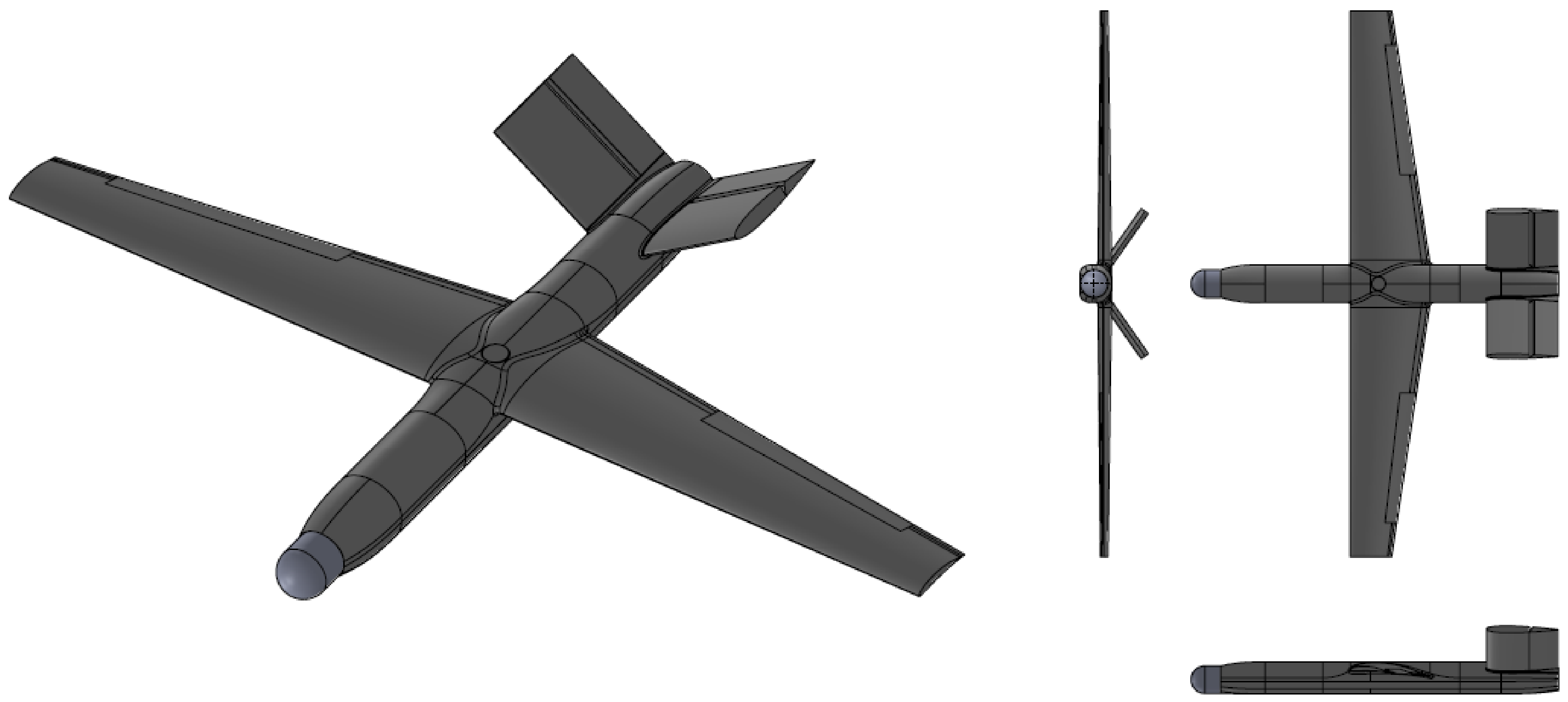
The design process begins with the definition of the mission flight characteristics and the operational requirements of the aircraft. Within the framework of this study, an Unmanned Aerial Vehicle (UAV) is selected as the case study, which was designed by the Applied Mechanics Laboratory at Mechanical Engineering and Aeronautics Department of the University of Patras, Greece. According to the NATO classification system for UAVs, the aircraft in this study falls into the Class I mini UAV category. Table 1 presents the key UAV parameters that serve as the basis for the aerodynamic optimization and design framework. The developed UAV is presented in Figure 1.

2.2. High-Fidelity CFD Aerodynamics

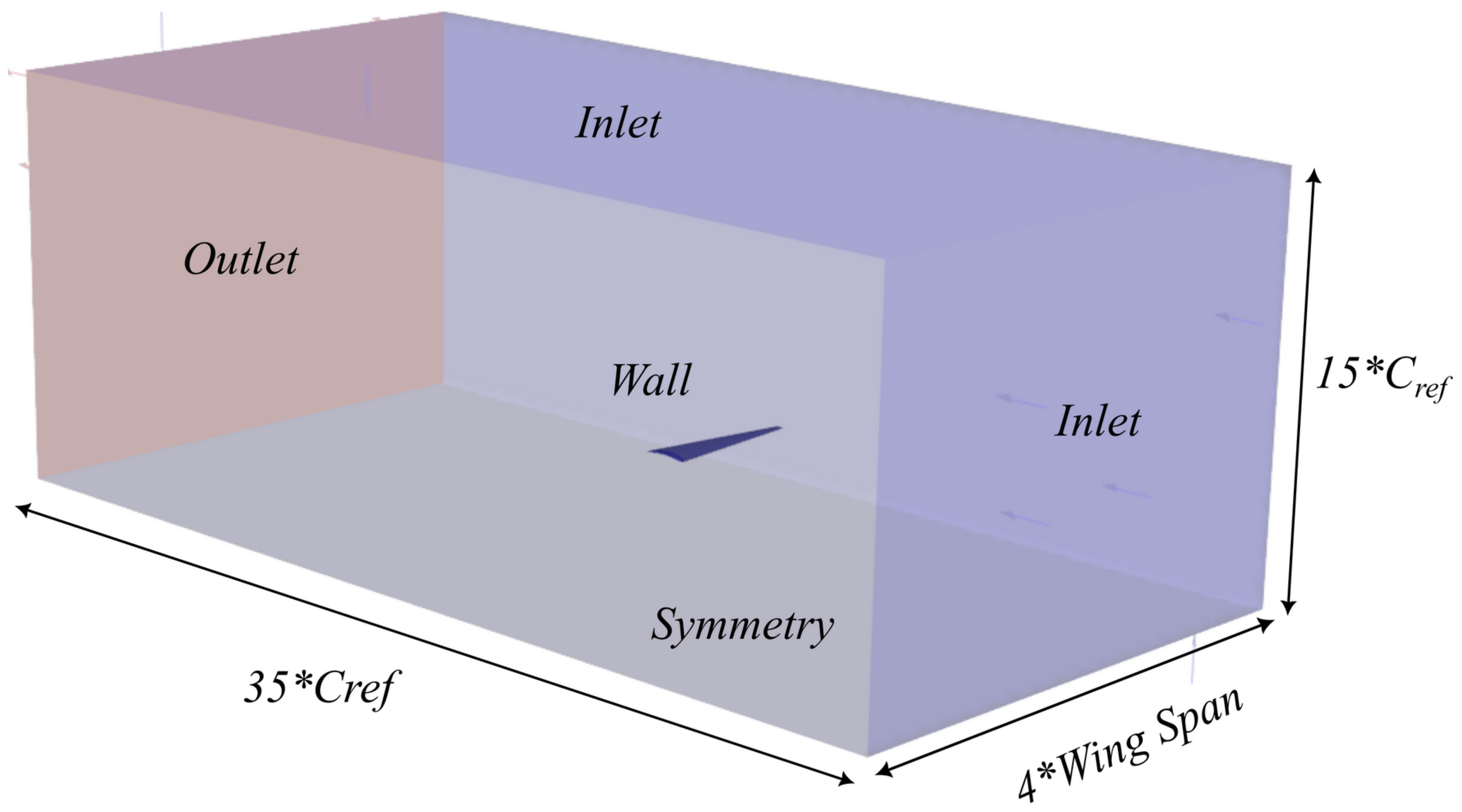
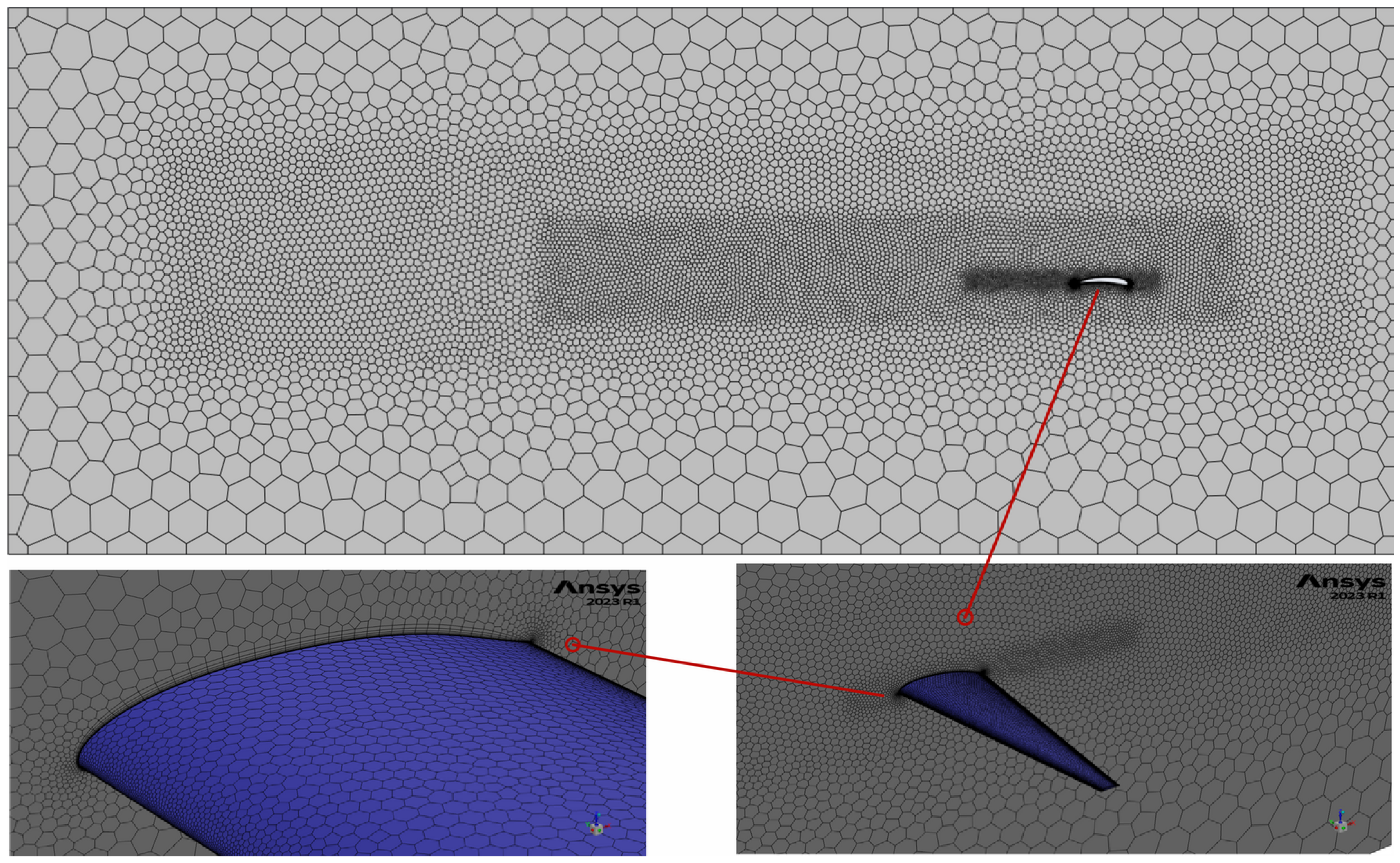
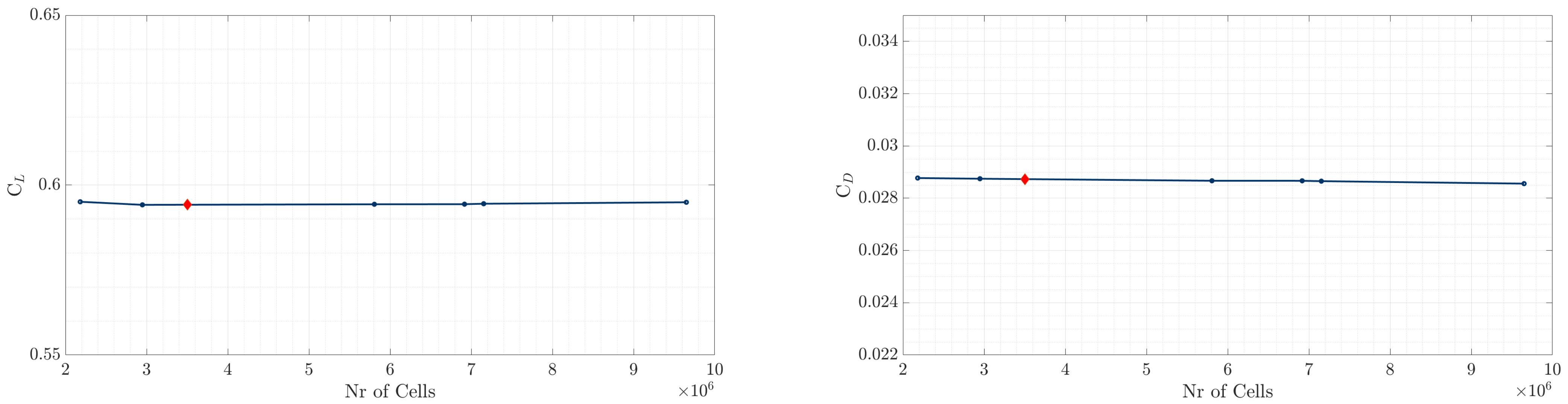
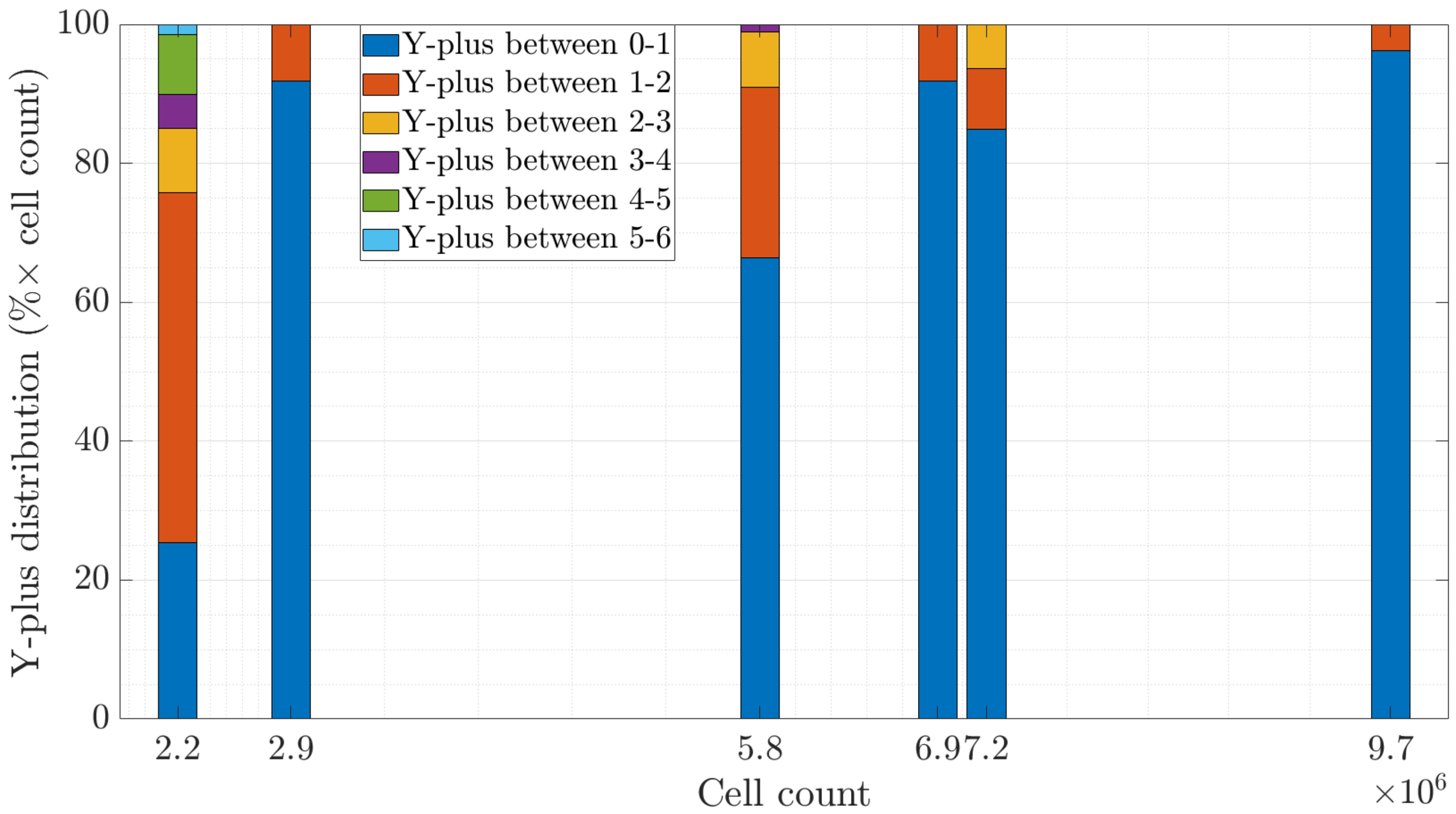
A numerical model of a wing, incorporating the average values of key geometric characteristics, was developed as the foundation for subsequent Computational Fluid Dynamics (CFD) analyses and optimization studies of various wing configurations derived from the surrogate model. The computational domain dimensions and boundary conditions were carefully designed to reflect the operational environment and altitude of the UAV. Simulations were conducted using ANSYS Fluent 2025R1 [28], solving the Reynolds-Averaged Navier–Stokes (RANS) equations coupled with the Spalart–Allmaras turbulence model [29]. The Spalart–Allmaras model was selected due to its robustness and proven performance in predicting attached and mildly separated flows at low Reynolds numbers, making it suitable for UAV aerodynamic analysis. The computational domain was defined as a rectangular region measuring 10.0 × 6.0 × 4.0 m. The RANS equations were discretized using the Finite Volume Method (FVM) under incompressible, steady-state flow assumptions with an appropriately refined mesh. To ensure accurate boundary layer resolution, a first cell wall distance of Y + 1 was achieved, with the initial layer height set to y = 7.4 × 10 5 m. A mesh independence study was also conducted to verify that further refinement did not impact the results, ensuring an optimal balance between accuracy and computational efficiency. The computational domain, including dimensions, boundary conditions, and mesh details, is illustrated in Figure 2 and Figure 3.
Pressure and temperature values were set according to the maximum operating altitude of the UAV, with a predefined inlet velocity. The outlet boundary conditions were defined with a zero pressure gradient, while the turbulence intensity was set to 1%. A symmetry boundary condition was applied along the longitudinal plane, and the wing surfaces were modeled as free-slip walls. The convergence of the lift and drag coefficients, C L and C D , respectively, is illustrated in Figure 4, while Figure 5 illustrates the Y + distribution for each model of the mesh independence study.

2.3. FEM Model

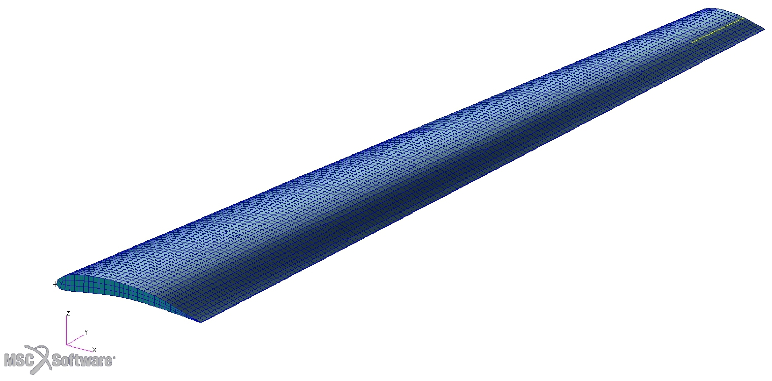
The FE model of the wing is generated based on the external surfaces of the UAV. The model is generated in MSC NASTRAN 2021 [30], and for the skins, spars, and ribs, 4-noded quadrilateral shell elements (CQUAD4) are used, and for the spar caps and stringers, beam elements (CBEAM), accounting also for the relevant offset values. As a datum design point, a cross-ply, two-layered laminate, consisting of a 0 and a 90 ply, is considered for all the relevant wing parts. The Hexcel IM7/8552 composite material system is selected for the relevant parts of the wing, with the respective B-Basis material properties, strength values and cured ply thickness listed in Table 2. For the beam elements and to simplify the analysis, rectangular cross-sections are considered. The respective thickness, nevertheless, is calculated based on the aforementioned laminate since they are also considered to be manufactured of the provided composite material. However, only isotropic materials are allowed for the definition of the CBEAM elements. As a result, and since the baseline lay-up is symmetric, equivalent laminate axial, bending and shear moduli, E e q a , E e q b and G e q respectively, can be calculated based on the following Equations (1) and (3) [31]:
E e q a = 1 t ( A 11 A 12 2 A 22 )
E e q b = 12 t 3 ( D 11 D 22 D 12 2 D 22 )
G e q = A 66 t
where t is the thickness, and A 11 , A 12 , A 2 , A 66 and D 11 , D 12 , D 22 are the corresponding terms of the extensional and bending stiffness matrix of a laminate. The equivalent modulus, E e q , is then selected as the minimum between the E e q a and E e q b values to ensure conservatism in the design. It should be noted that the use of equivalent isotropic properties for the CBEAM elements neglects anisotropic coupling effects of composite laminates, such as bend–twist coupling (associated with non-zero D 16 and D 26 terms). However, the baseline laminate considered here is symmetric and cross-ply, for which such coupling effects are inherently negligible. This assumption is therefore considered appropriate for preliminary structural sizing and for maintaining computational efficiency within the surrogate-based optimization framework. Regarding the boundary conditions, the wing is assumed to be clamped at its root section, thus fixing all relative nodal Degrees of Freedom (D.o.F). The resulting FEM mesh of the wing model is presented in Figure 6.

2.4. Surrogate Modeling

The key steps in a typical SBO process, as outlined in Alexandrov et al. [33], include:
  • Sampling the design space and evaluating the objective function along with any constraints.
  • Constructing the surrogate model based on the sampled data.
  • Searching the design space and refining the surrogate model using update (infill) criteria.
  • Enhancing the model by incorporating newly added points and repeating the process.
The sampling stage is a crucial step in an SBO algorithm, as the surrogate model’s accuracy depends on the selection of initial design points. To ensure the model represents the design space effectively, the most influential points must be chosen to maximize the information available for surrogate construction. Given the often high-dimensional nature of design problems, exhaustive grid searches become computationally prohibitive. Instead, more efficient techniques, such as Latin Hypercube Sampling (LHS) [34], are commonly used. LHS is a robust statistical method that generates parameter samples from a multidimensional distribution while maintaining a well-distributed design space representation. The method involves an optimization problem aimed at maximizing the distance between sample points while ensuring each coordinate follows a predefined probability distribution. Once the sampling is completed, the next step is to construct the surrogate model, typically represented as a general function:
f ^ ( x , w )
where w denotes model parameters, and x represents the design variables. A key criterion for selecting a surrogate model is its ability to accurately capture the desired function’s characteristics while maintaining flexibility. Overly rigid models risk instability and overfitting. One widely used surrogate model in engineering applications is Kriging [35,36], which expresses function approximations as a linear combination of basis functions (kernels) that depend on the Euclidean distance between design points. For noise-free data, the Kriging approximation is given by
f ^ ( x ) = i = 1 N w i ψ x x ( i )
where:
  • N c is the number of basis functions;
  • x c ( n ) represents the center of the n-th basis function;
  • ψ ( | | x x c ( n ) | | ) is the kernel function, evaluated based on the distance between the prediction point x and the corresponding center.
The kernel function is typically defined as
ψ x x ( i ) = exp k = 1 d θ k x k x k ( i ) p k
where θ n and p n are model parameters.
The Kriging model is constructed using the following steps:
  • Formulating the correlation matrix based on training data points:
    [ Ψ ] i j = exp k = 1 d θ k x k ( i ) x k ( j ) p k
  • Maximizing the Maximum Likelihood Estimator (MLE):
    ln ( M L E ) = n 2 ln ( σ ^ 2 ) 1 2 ln ( [ Ψ ] )
    where σ ^ is the MLE estimate of the standard deviation.
  • Predicting values at new design points:
    y ^ ( x ) = μ ^ + r T ( x ) Ψ 1 ( y 1 μ ^ )
where r ( x ) is the correlation vector between the prediction point and the sampled data points. For Gaussian-based processes, the Mean Square Error (MSE) estimation is given by
s ^ ( x ) 2 = σ ^ 2 1 ψ T [ Ψ ] 1 ψ + 1 1 T [ Ψ ] 1 ψ 1 T [ Ψ ] 1 1
A commonly used approach for improvement is the Expected Improvement (EI) function:
E [ I ( x ) ] = ( y min y ^ ( x ) ) Φ y min y ^ ( x ) s ^ ( x ) + s ^ ( x ) ϕ y min y ^ ( x ) s ^ ( x )
where Φ and ϕ denote the cumulative distribution and probability density functions, respectively. As an additional step toward more realistic SBO frameworks, constraints should be incorporated into the surrogate model. The approach to constraint handling depends on the computational cost of evaluating the constraint function. Constraints can either be evaluated directly or modeled using surrogate techniques similar to those applied to the objective function, effectively creating a surrogate model for each constraint. When constraint evaluations are computationally inexpensive, conventional constraint optimization methods, in conjunction with the objective function surrogate model, guide the SBO framework toward both promising and feasible regions of the design space. However, if surrogate models are also employed for constraints, the Expected Improvement function from Equation (11) is modified into the constrained Expected Improvement function by introducing the probability of feasibility:
P [ F ( x ) ] = Φ 0 g ^ ( x ) s ^ g ( x )
where F represents the feasibility measure of a constraint g, and s g ^ denotes the variance of the constraint’s Kriging model. The probability of achieving an improvement over the current minimum function value while satisfying feasibility conditions is then determined by multiplying Equations (11) and (12):
E [ I ( x ) F ( x ) ] = E [ I ( x ) ] · P [ F ( x ) ]
To determine the next point for model refinement, a sub-optimization problem is solved:
x infill = arg max ( E [ I ( x ) ] · P [ F ( x ) ] )
This function depends on the Kriging model parameters, θ n and p n ; while optimizing both the correlation length parameters, θ n and the exponents p n can improve prediction accuracy in many applications, and doing so increases the complexity of the optimization process. To simplify the model calibration and reduce computational costs, we follow the approach commonly adopted in the surrogate modeling literature [35,36,37] and fix the value of p n = 2 , corresponding to a Gaussian correlation function. This allows us to focus on tuning θ n alone, using a global optimization method, which, in our case, is a genetic algorithm, as implemented in Python 3.14. The particular optimization was executed for 1000 iterations. As noted by Forrester et al. [37], searching for θ n on a logarithmic scale, typically within the bounds 10 3 to 10 2 , is effective. It is also recommended to scale the input design space to [0, 1] to ensure consistent interpretability of the parameter values across different problems.
The resulting point, x infill , is then added in the current dataset, which is then re-trained. This process is typically repeated for a predefined number of iterations. Within the present study, a samples-to-infill points ratio of 1:2 was selected as recommended in [36]. This ensures that the surrogate model is updated efficiently, balancing exploration and exploitation for improved optimization performance.

2.5. High-Fidelity Aerostructural SBO Framework

The SBO framework employs high-fidelity analysis tools and is executed using five distinct DoE strategies. Following a previous study by the authors, multiple wing configurations are generated using the selected optimized airfoil [27]. The objective of the SBO framework is to identify the optimal aerostructural wing geometry that maximizes the range R, (Equation (15)) of the specific aircraft, subject to constraints on the cruise lift coefficient, static strength and stiffness (global buckling).
R = 3.6 g · L D · E s b η b 2 s η p m b m
where:
  • m b = mass of batteries [kg]
  • m = aircraft total mass [kg]
  • E s b = battery specific energy [Wh/kg]
  • η p = propeller efficiency
  • η b 2 s = total system efficiency from battery to motor output shaft
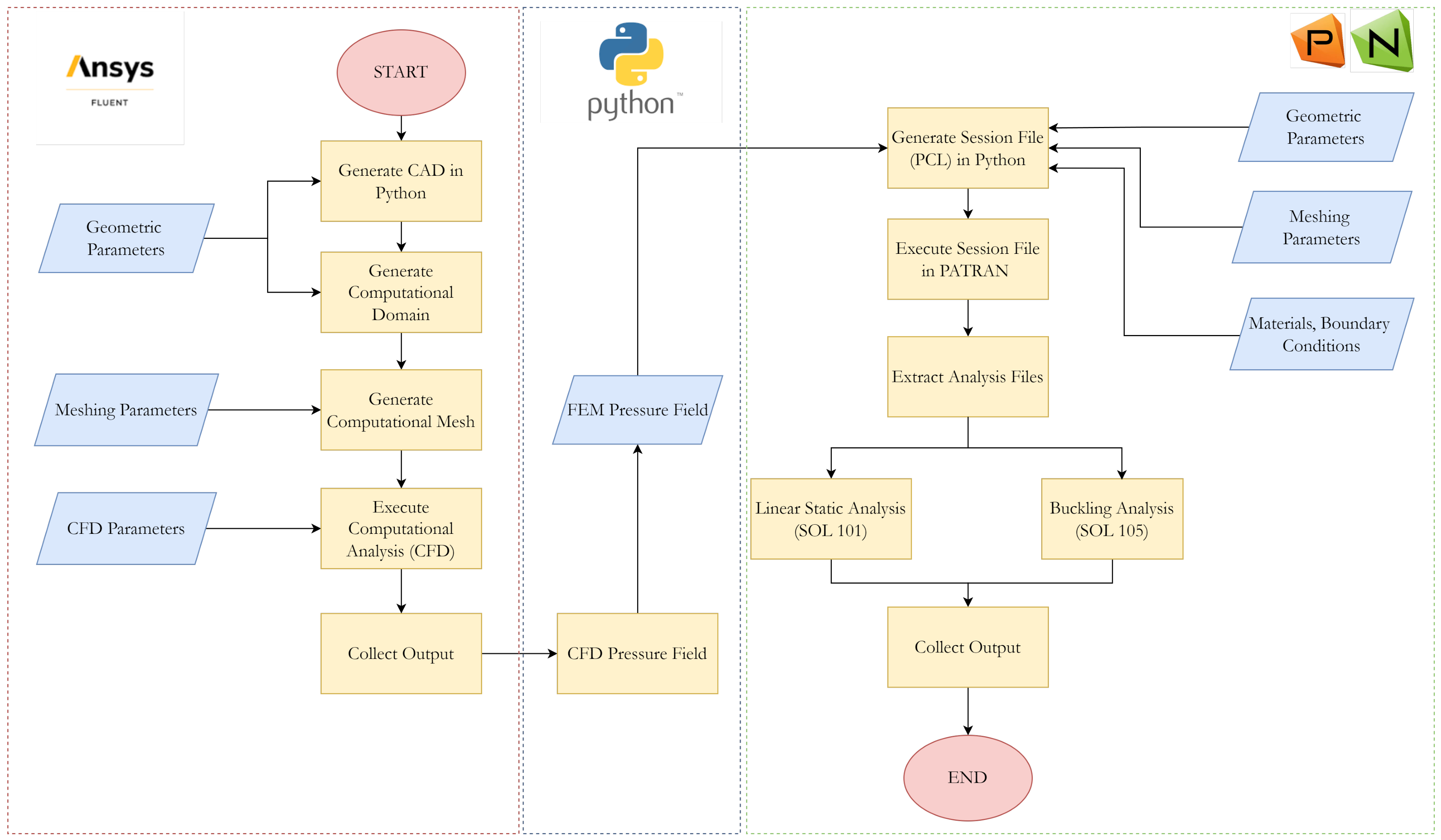
The optimization considers twelve key geometric design variables, comprising four aerodynamic parameters—aspect ratio, taper ratio, sweep angle, and tip twist—and eight structural parameters, including skin thickness, rib thickness, front spar thickness, rear spar thickness, rib spacing, stringer spacing, front spar location, and rear spar location. Each DoE consists of 120 wing models generated within the defined design space. Based on these samples, the SBO framework is trained and subsequently used to generate an additional 60 candidate wing configurations, with the objective of identifying the most suitable design that satisfies the imposed constraints while maximizing range. At the conclusion of each SBO iteration, an optimized wing configuration is obtained, and the resulting optimal designs from the five DoEs are finally compared to assess consistency and robustness of the optimization results. At each SBO iteration the framework starts from the generation of the geometry of the wing, the subsequent computational domain and CFD mesh. The CFD analyses are then conducted, and output is collected in terms of the lift constraint as well as the pressure field in the skins of the wing. Moving to the FEM modeling framework, interpolation schemes are used to map the pressure field from the CFD to the FEM mesh. It should be noted that the present framework adopts a one-way coupling strategy, where aerodynamic loads are transferred from CFD to the structural model without deformation feedback to the aerodynamic solver. Preliminary aeroelastic analyses performed at the design stage using low-fidelity methods indicated that deformation effects on aerodynamic performance are not dominant for the considered configuration. Therefore, the one-way coupling assumption is considered appropriate for the present preliminary design framework. Given the geometric parameters of the wing, Patran Command Language (PCL) scripts are used to generate a new wing geometry and mesh. Subsequently, the analysis files (linear static and global buckling) are extracted and executed, followed by output collection in terms of strength and stiffness constraints. The overall flowchart of the framework is presented in Figure 7.
A summary of all variables, including their lower and upper bounds, is given in Table 3. A horizontal line is used to separate aerodynamic from structural variables. The overall optimization problem setup is summarized in Table 4.
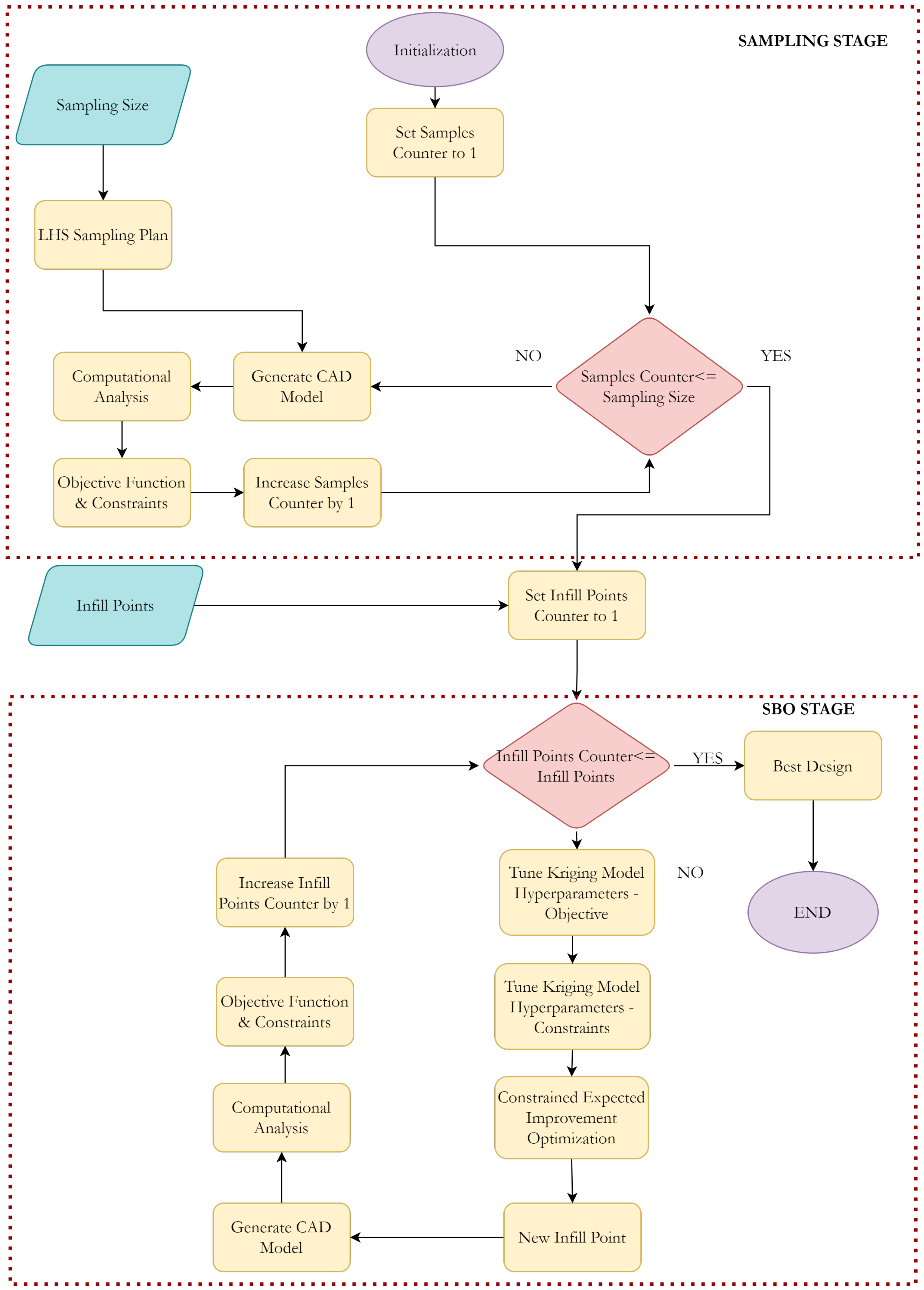
The SBO framework, as illustrated in Figure 8, is common to the previous framework and consists of two main stages: the sampling stage and the model updating stage. The process begins with the definition of the sampling size, followed by generating samples using the LHS method. Subsequently, the geometry and mesh of the geometry are generated and further analyzed via each computational tool. The objective and constraint functions are then obtained for each sample. Once the training stage is completed, the main SBO framework is initiated. The hyperparameters of the Kriging model representing the objective and constraint functions are determined. Next, the constrained Expected Improvement function (Equation (13)) is minimized using a sub-optimization routine, yielding a new point in the design space. The computational analysis is then performed for this new point, and the surrogate model is updated accordingly. This iterative process continues for a predefined number of infill points.

3. Results

3.1. Surrogate Model Accuracy

The predictive accuracy of the surrogate models was assessed using the Root Mean Square Error (RMSE) and the coefficient of determination ( R 2 ). These metrics were evaluated using the infill points generated during the optimization process, which serve as an independent validation dataset. They quantify the average prediction error and the overall agreement between the predicted ( y ^ i ) and high-fidelity ( y i ) responses, and are defined as
RMSE = 1 N i = 1 N y i y ^ i 2
R 2 = 1 i = 1 N y i y ^ i 2 i = 1 N y i y ¯ 2
where N denotes the number of validation points and y ¯ is the mean of the corresponding high-fidelity responses. A low RMSE and an R 2 value approaching unity indicate high predictive accuracy of the surrogate model.
The results for five independent SBO runs are summarized in Table 5.
Overall, the surrogate models achieved a mean RMSE of 5.62 with a standard deviation of 1.11 . For four out of five runs (Runs 2–5), the coefficient of determination remains consistently high ( R 2 > 0.90 ), indicating a strong correlation between the surrogate predictions and the corresponding high-fidelity responses.
In contrast, Run 1 exhibits a significantly lower R 2 value, despite having an RMSE of comparable magnitude to the other runs. This behavior is attributed to the relatively narrow range of objective function values in the corresponding infill dataset, where the range varies approximately between 190 km and 208 km, resulting in a reduced variance of the reference data. Since the R 2 metric depends on the ratio S S r e s / S S t o t , a small variance increases its sensitivity to moderate absolute prediction errors. As a result, even moderate absolute prediction errors lead to a disproportionately low (or negative) R 2 value.
This behavior is commonly observed in surrogate-based optimization when validation points are concentrated near optimal regions. Therefore, the RMSE provides a more reliable indicator of predictive performance in this case. In particular, the normalized RMSE for Run 1 is approximately 2.9 % of the mean range value, indicating that the absolute prediction error remains moderate. Considering the consistently low RMSE values across all runs, the surrogate models are shown to provide an accurate approximation of the high-fidelity response, ensuring reliable performance within the surrogate-based optimization framework. This interpretation is further supported by the Leave-One-Out (LOO) cross-validation results presented below, which demonstrate consistent surrogate accuracy across all runs.
To further evaluate the generalization capability of the surrogate model, a LOO cross-validation analysis was performed. In this approach, each sample in the DoE is temporarily excluded from the training set, and the model is reconstructed using the remaining N 1 samples. The excluded point is then predicted, and the corresponding prediction error is recorded. This process is repeated for all N samples, providing a robust estimate of model accuracy while reducing the risk of overfitting. The LOO Root Mean Square Error ( RMSE LOO ) is computed as
RMSE LOO = 1 N i = 1 N y i y ^ i , LOO 2
where y ^ i , LOO denotes the prediction obtained by excluding the i-th sample from the training set. In addition, the corresponding coefficient of determination, R LOO 2 , was also evaluated in order to quantify the overall agreement between the cross-validated predictions and the high-fidelity responses.
The computed values for the five independent SBO runs are summarized in Table 6.
The LOO errors are highly consistent across all runs, with a mean RMSELOO of 8.31 × 10 0 and a mean R LOO 2 of 0.818 ± 0.006 . The relatively small standard deviation of both metrics indicates stable surrogate behavior across the independent SBO runs. Although some isolated samples exhibit larger local deviations, as reflected by the maximum absolute errors, the overall cross-validation performance confirms that the Kriging surrogate provides a reliable approximation of the high-fidelity response throughout the sampled design space.

3.2. Best Configurations of All Five SBO Iterations

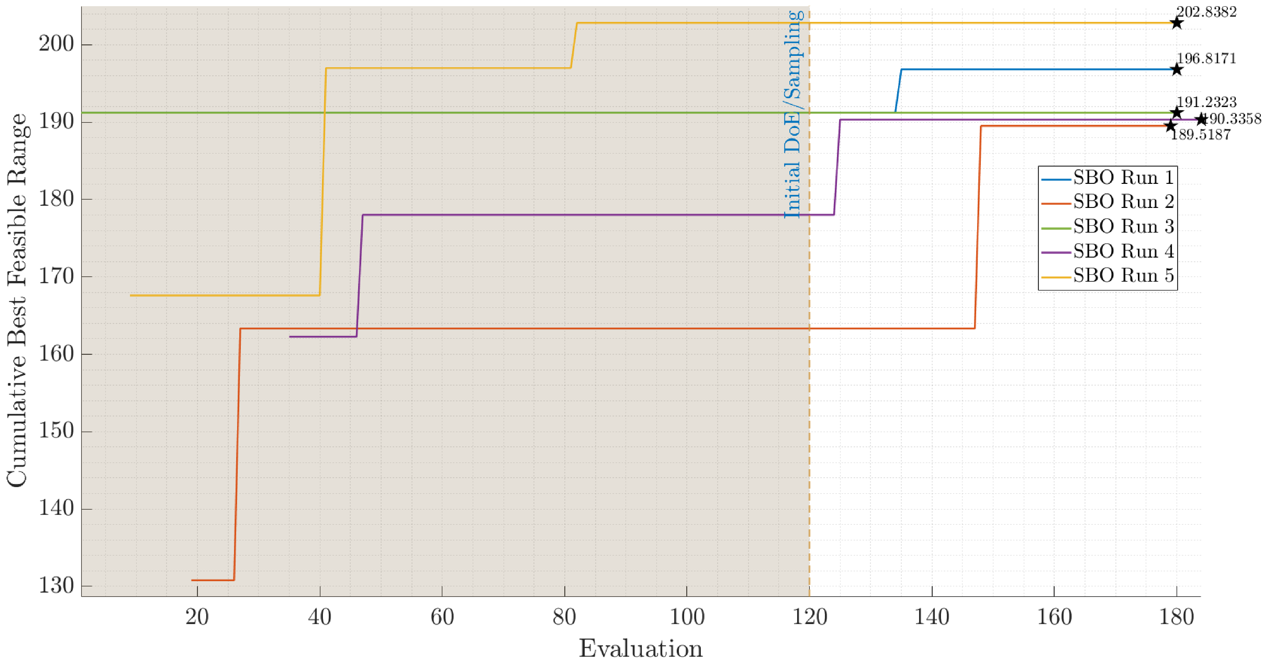
In this subsection, the best feasible configurations from each SBO iteration are presented and compared to each other. Figure 9 illustrates the convergence history of the cumulative best feasible range (R) for the five SBO iterations. Among the runs, the fifth SBO iteration achieves the highest final range (≃202.8), followed by the first iteration (≃196.8), whereas the second, third and fourth iterations converge to similar intermediate values (≃189–191).
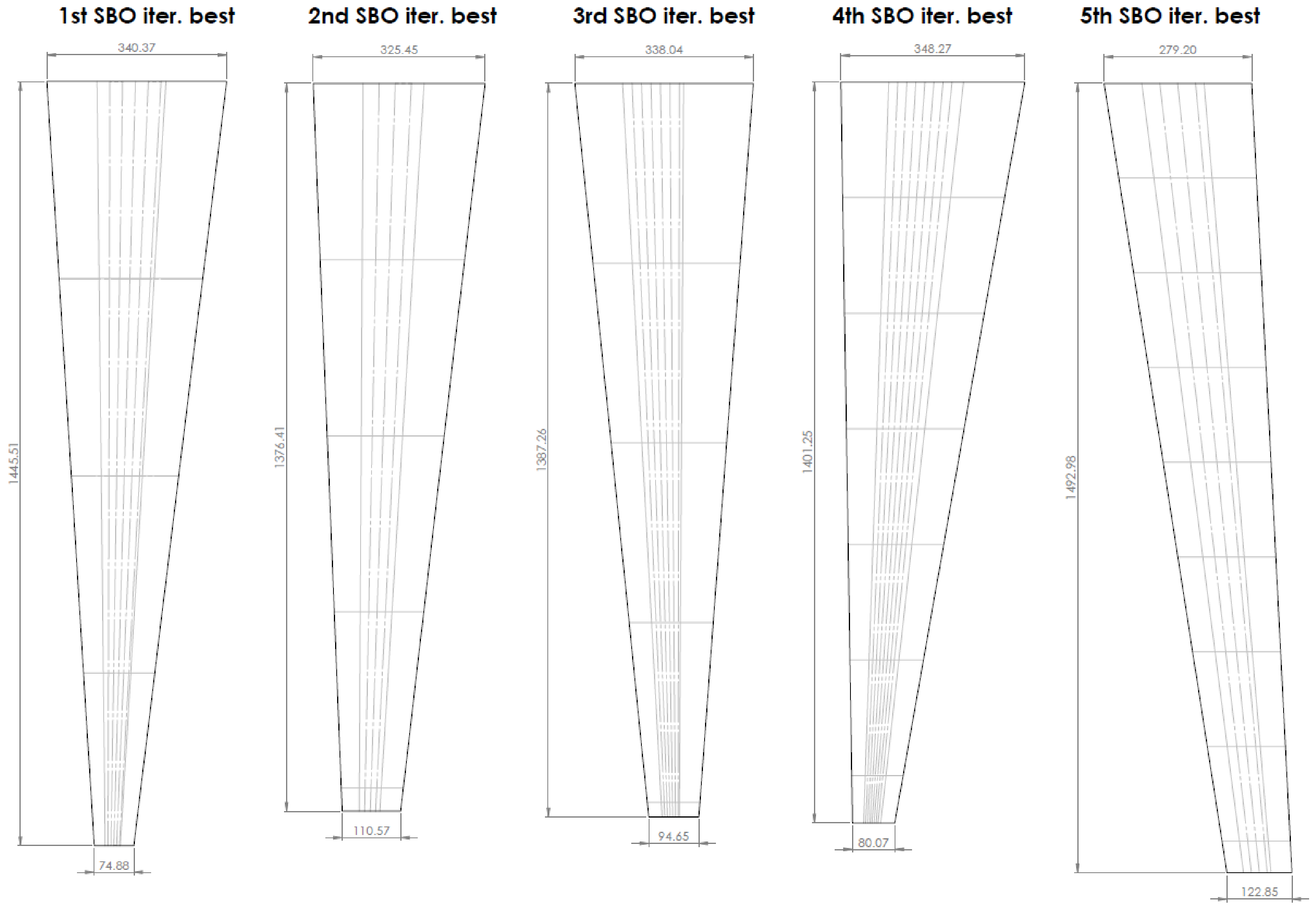
Table 7 presents the optimal configurations obtained at each SBO iteration, along with their corresponding aerodynamic and structural design parameters. All five configurations exhibit high lift-to-drag ratios ( L / D > 25.5 ), while the weight remains nearly constant across all cases ( W 0.83 ), indicating that performance improvements are primarily driven by aerodynamic efficiency. Regarding the constraints, g 1 and g 4 are negative and close to zero, confirming that they are active and govern the feasible boundary of the optimization. The dominance of constraints g 1 and g 4 can be explained by their direct relationship with structural sizing. Constraint g 1 (strength) is governed by the stress levels induced by aerodynamic loads, which increase with lift generation and aspect ratio. Constraint g 4 (buckling) is primarily driven by panel thickness and structural stiffness, and becomes critical as the optimizer reduces thickness to improve aerodynamic performance. As a result, these constraints define the boundary of the feasible design space. Near this boundary, small variations in thickness or load-related parameters can lead to significant changes in constraint values, resulting in a narrow feasible region. Consequently, the optimal solutions tend to lie close to the intersection of these constraints, reflecting the trade-off between aerodynamic efficiency and structural integrity. In contrast, g 2 and g 3 remain significantly negative, indicating that they are inactive and do not influence the optimal solutions. From an aerodynamic design perspective, all configurations are characterized by relatively high aspect ratios, with the fifth design achieving the largest value ( A R = 14.86 ), approaching the upper bound of the design space. The taper ratio and sweep angle remain moderate ( λ < 0.44 and Λ < 10 ), while tip twist varies between 0 . 40 and 2 . 11 , reflecting adjustments in load distribution and aerodynamic performance. In terms of structural design, the parameters are generally consistent across all configurations, with the most notable variations observed in rib spacing (RS) and stringer spacing (SS), suggesting that these variables play a key role in accommodating the aerodynamic changes while maintaining structural feasibility.
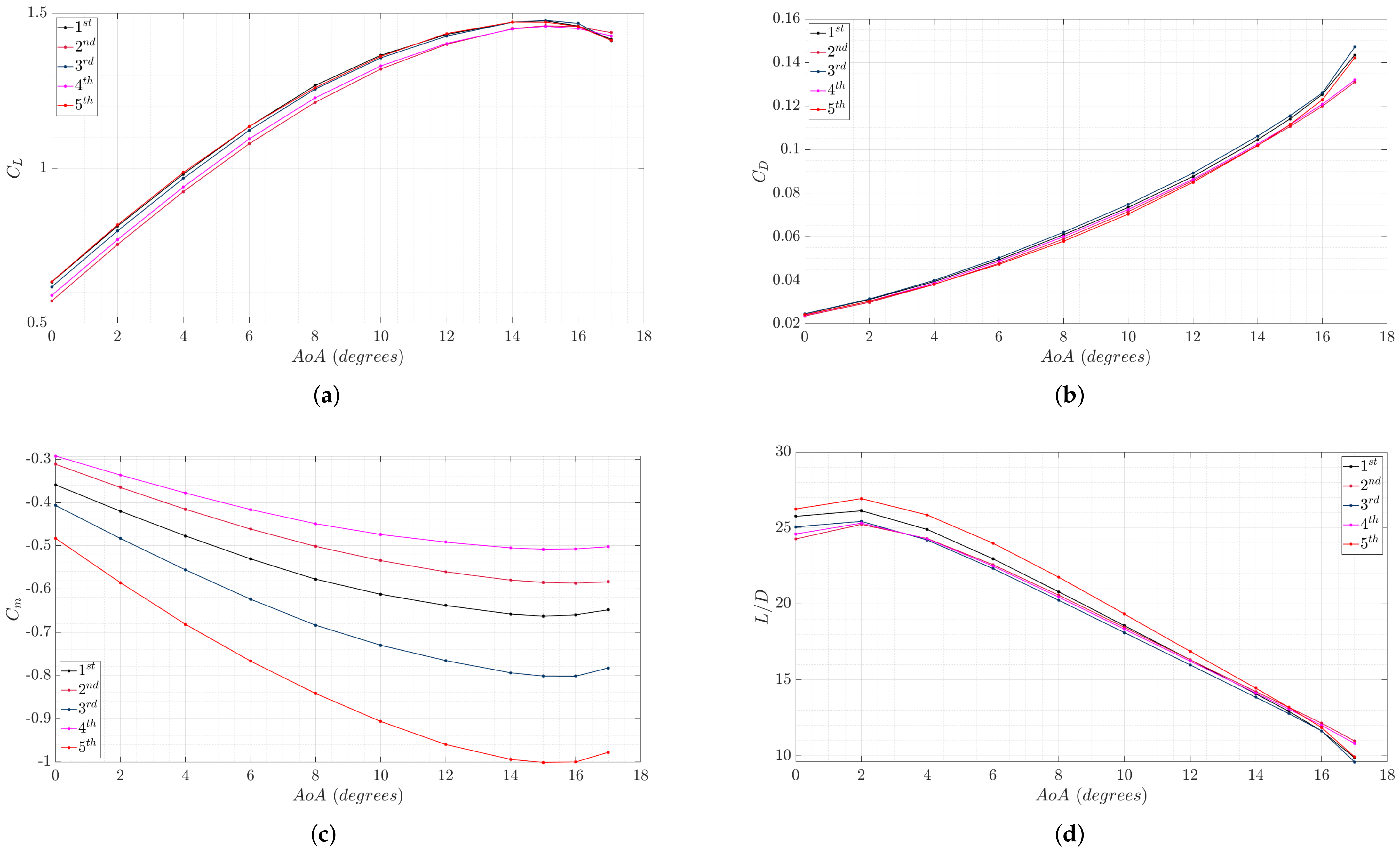
Figure 10 illustrates the planform geometry of the five best wing configurations, including their key dimensions: semi-span ( b / 2 ), root chord ( C r o o t ), and tip chord ( C t i p ) but also the ribs, spars (grey lines) and stringers (grey dashed lines). Figure 11 presents the corresponding aerodynamic performance obtained from CFD analyses, including the variations of lift coefficient ( C L ), drag coefficient ( C D ), moment coefficient ( C m ), and lift-to-drag ratio ( L / D ) with angle of attack (AoA). Among the configurations, the fifth wing demonstrates the best overall aerodynamic performance. It achieves the highest lift-to-drag ratio and maintains superior behavior across the entire AoA range, indicating improved aerodynamic efficiency and stability characteristics compared to the other designs.
Therefore, the fifth wing configuration is selected as the optimal design, as it demonstrates superior performance among the five candidates. It achieves the maximum range of ≃203 km while also exhibiting the best overall aerodynamic characteristics. In addition, it satisfies all the constraints imposed in the SBO optimization process.

3.3. Selected Optimized Configuration

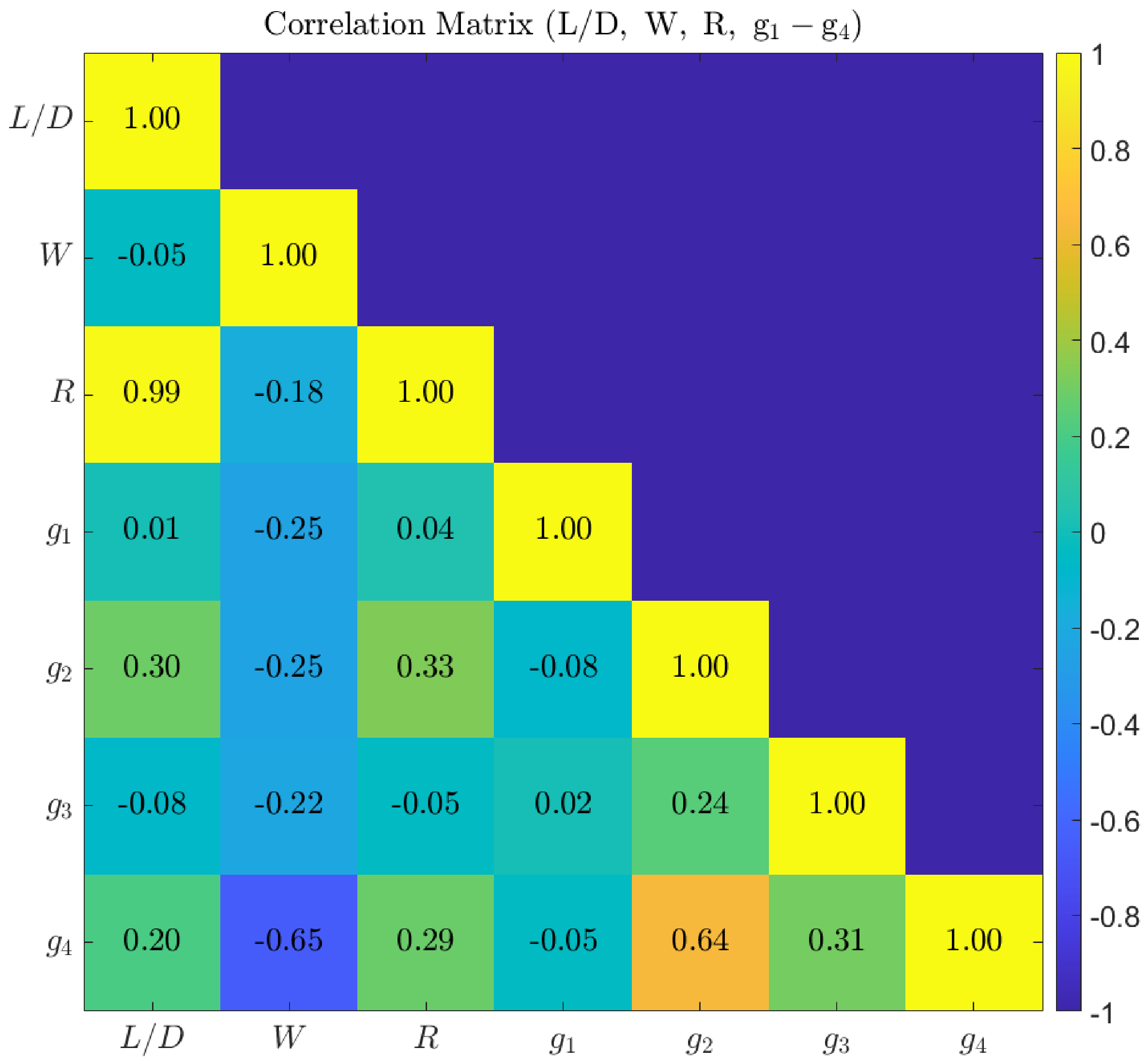
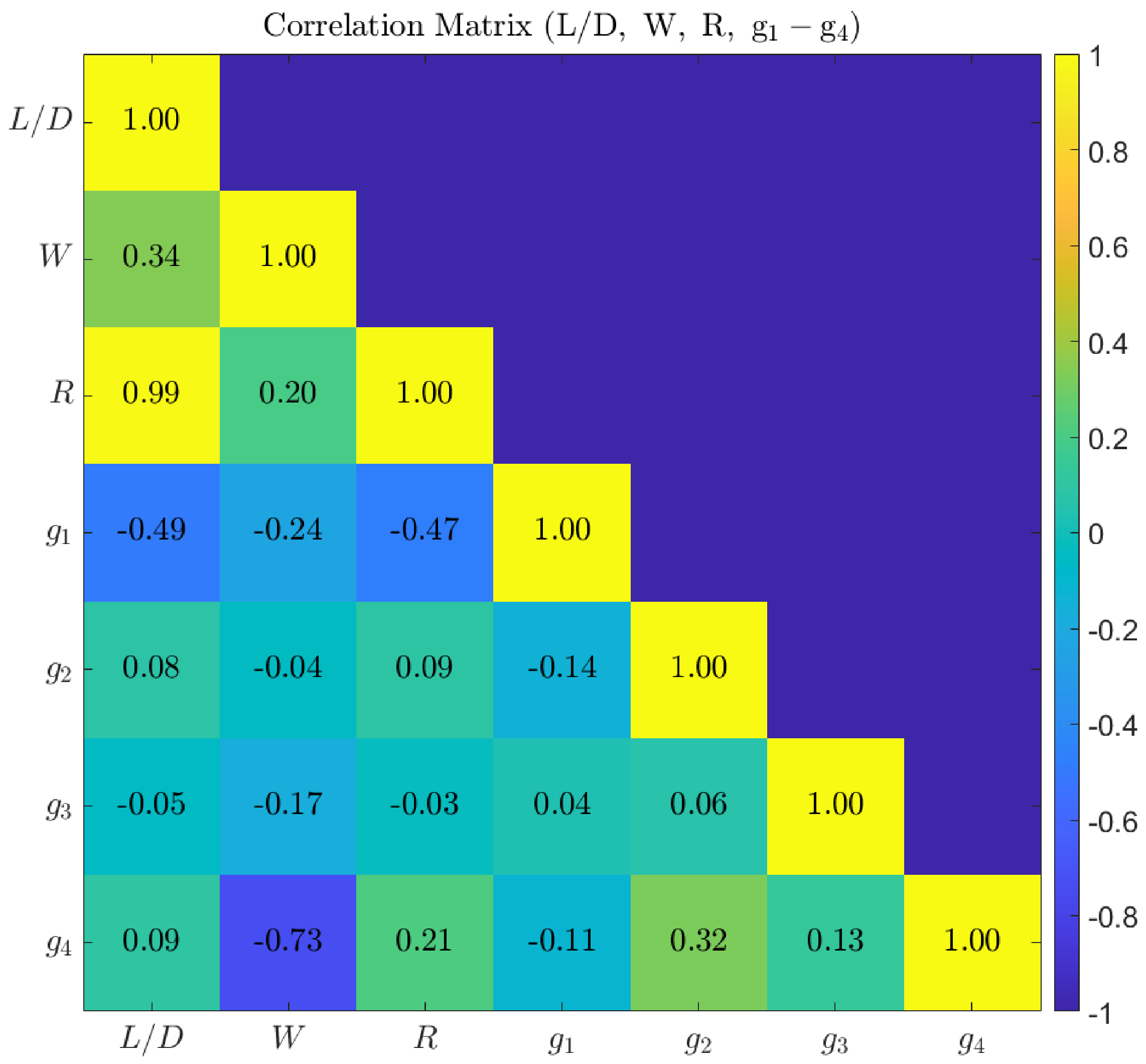
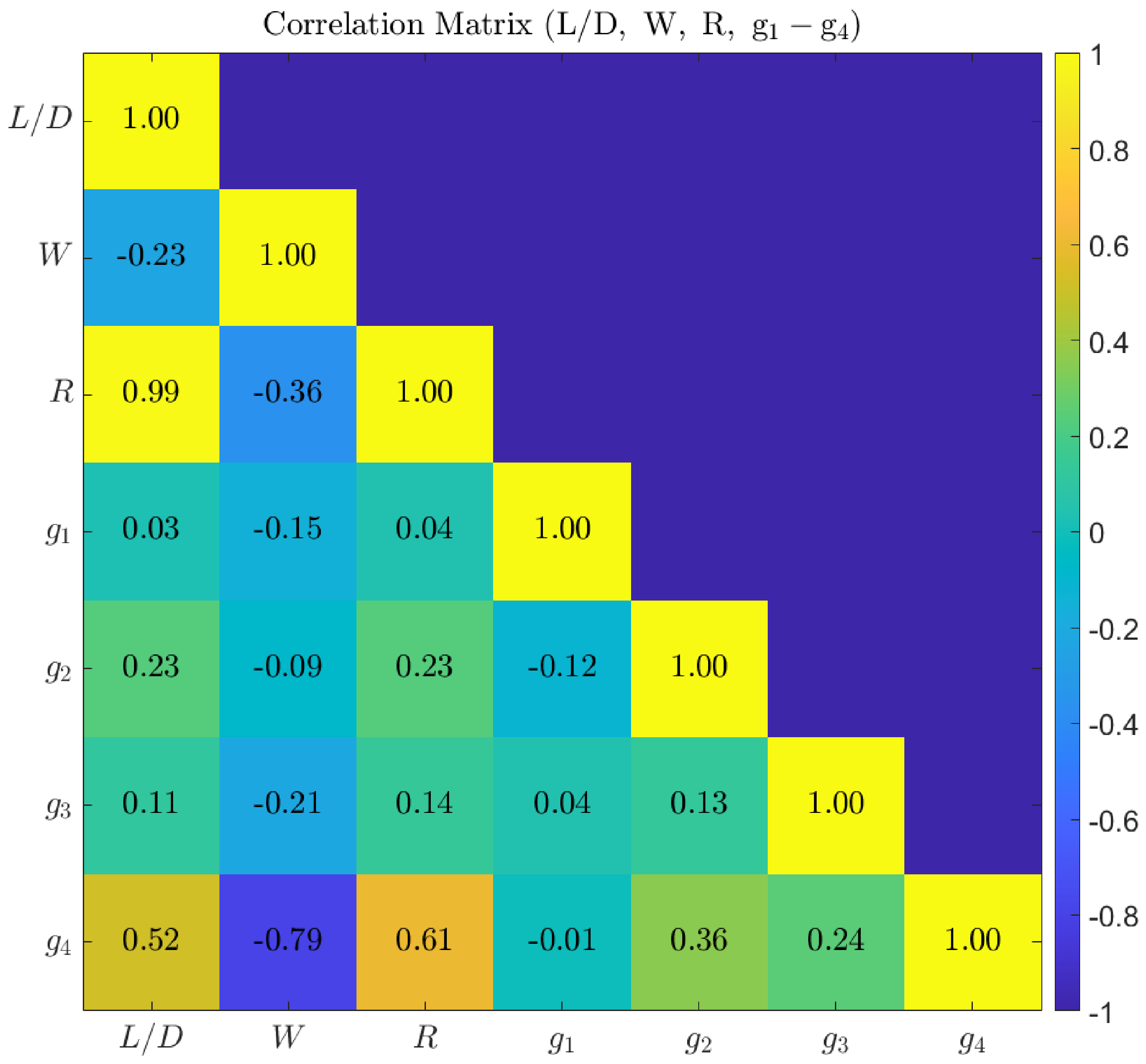
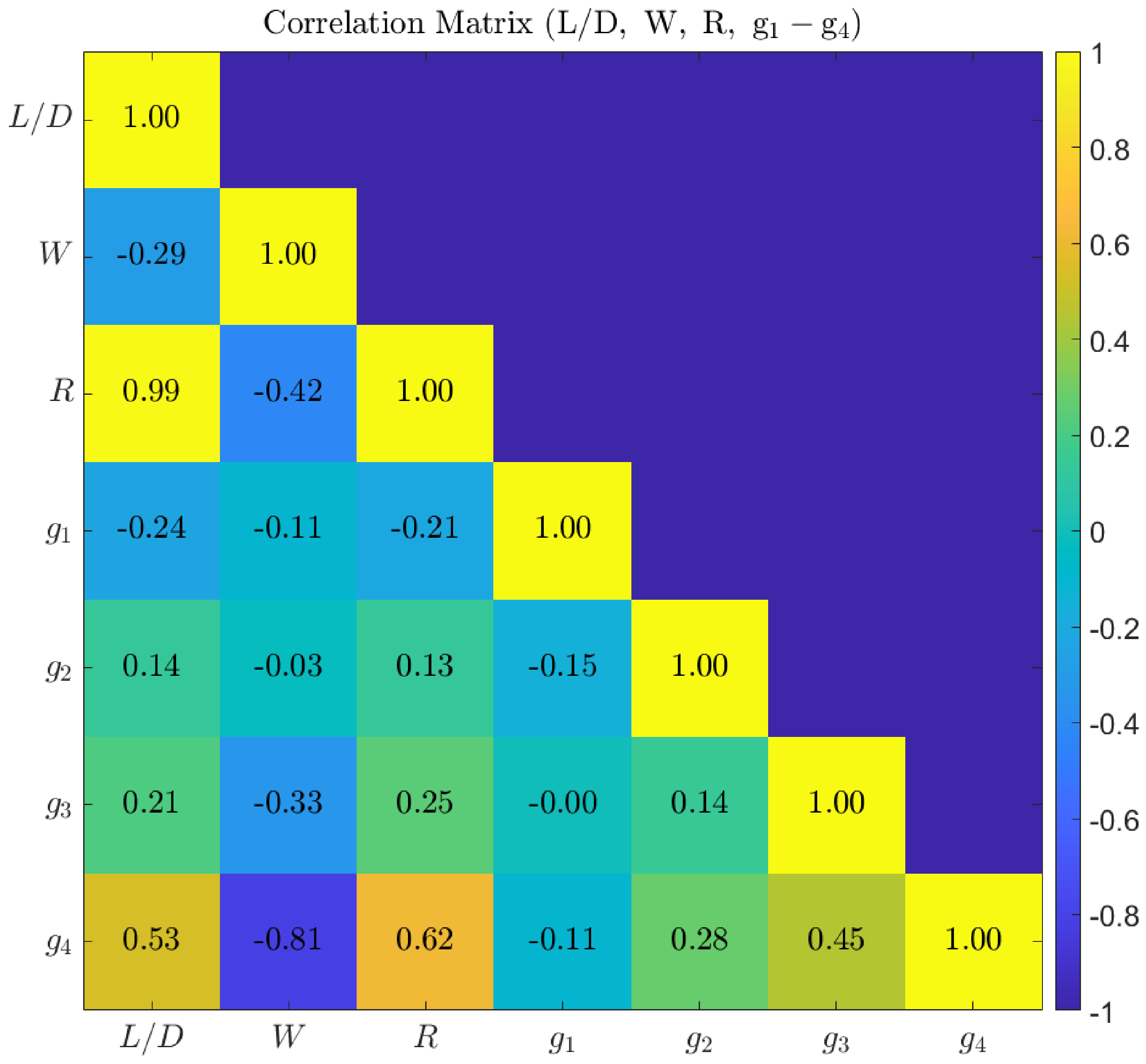
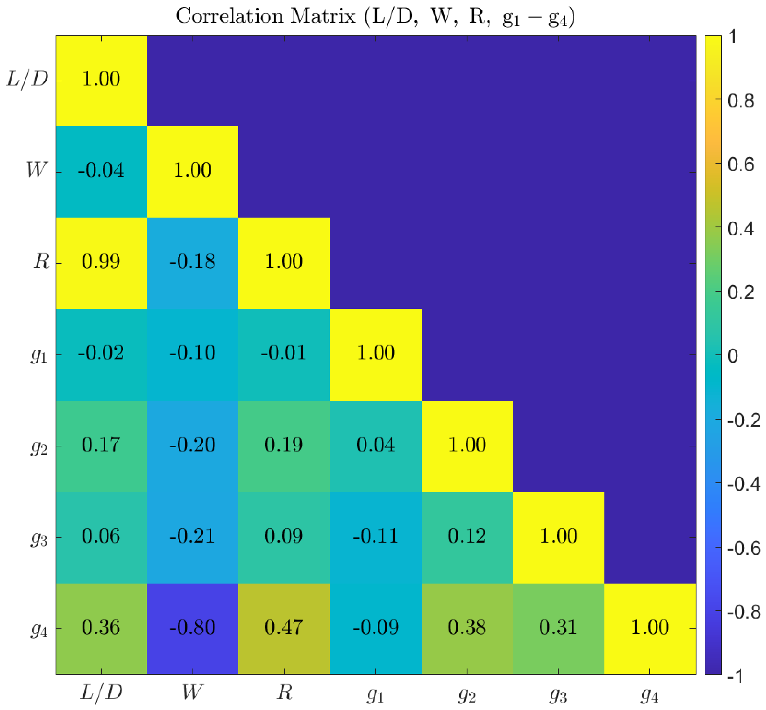
In this subsection, the results of the fifth SBO iteration are presented, from which the best optimized wing configuration was selected. In addition, the results of the aerodynamic and structural analyses of the optimized wing are presented. Figure 12 presents the correlation matrix for the final dataset after incorporating all samples and infill points, providing a consolidated view of the relationships among the performance variables and constraints. As observed in all previous iterations (Figure A1, Figure A5, Figure A9 and Figure A13), L/D and R maintain a nearly perfect positive correlation (0.99), confirming that aerodynamic efficiency consistently dominates range performance throughout the optimization process. The correlation between weight and the performance variables remains weakly negative, with W showing correlations of −0.05 with L/D and −0.18 with R, indicating that, within the explored design space, variations in weight have a relatively limited influence on range compared to aerodynamic efficiency. The constraint correlations remain generally weak with respect to the primary performance variables. Constraint g 1 shows almost no correlation with L/D(0.01) and R(0.04), while maintaining a modest negative correlation with weight (−0.25), suggesting limited coupling with the main design variables. Constraint g 2 exhibits slightly stronger positive correlations with L/D(0.30) and R(0.33), indicating a mild dependence on aerodynamic performance, while g 3 continues to show weak correlations with all variables. Among the constraints, g 4 remains the most strongly influenced by the design variables, displaying a moderate negative correlation with weight (−0.65) and moderate positive correlations with R(0.29) and g 2 (0.64). Overall, the final correlation structure confirms that aerodynamic efficiency is the primary driver of range, while most constraints remain weakly coupled to the performance variables, with g 4 showing the most noticeable dependency within the constraint set.
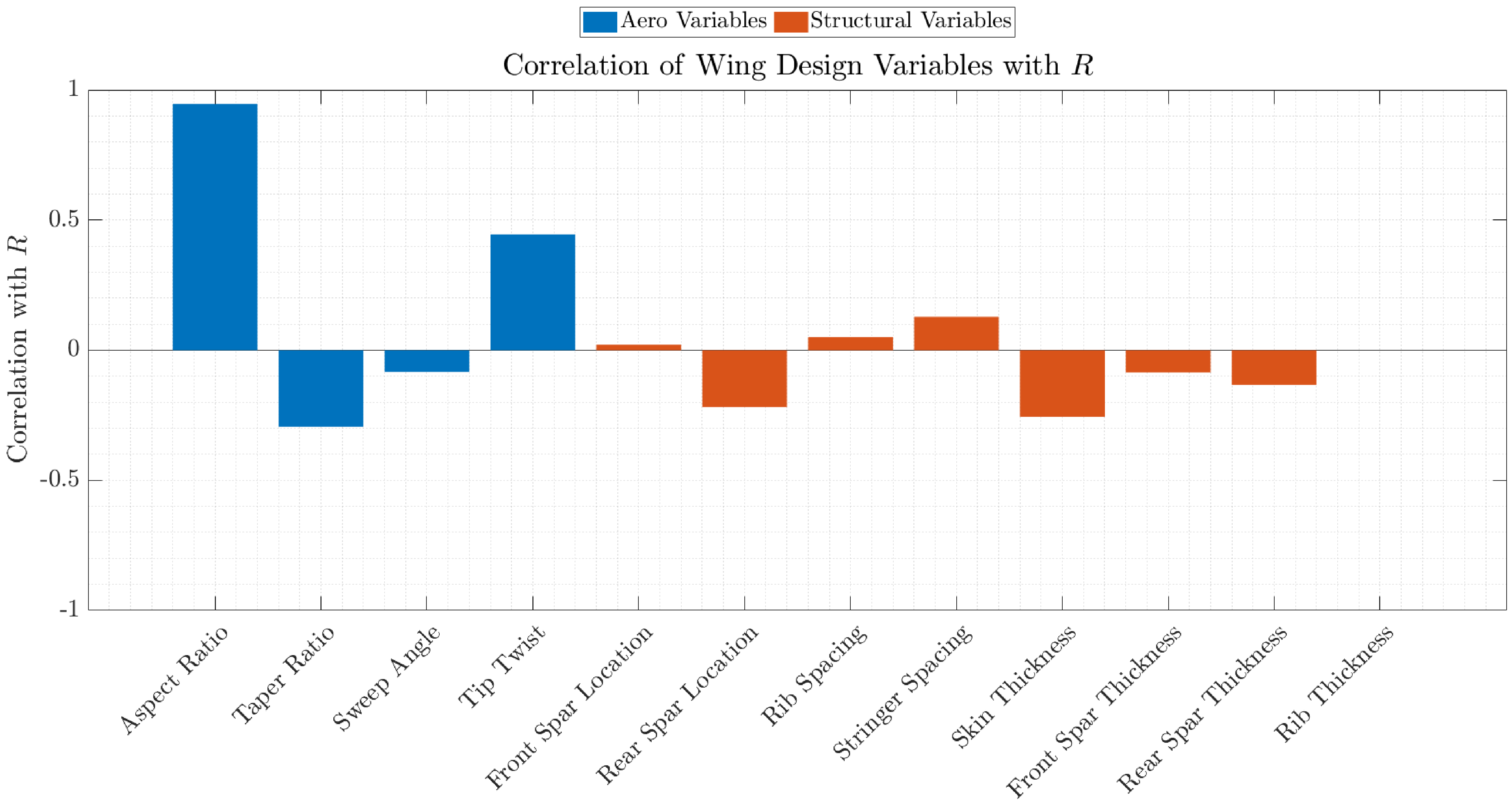
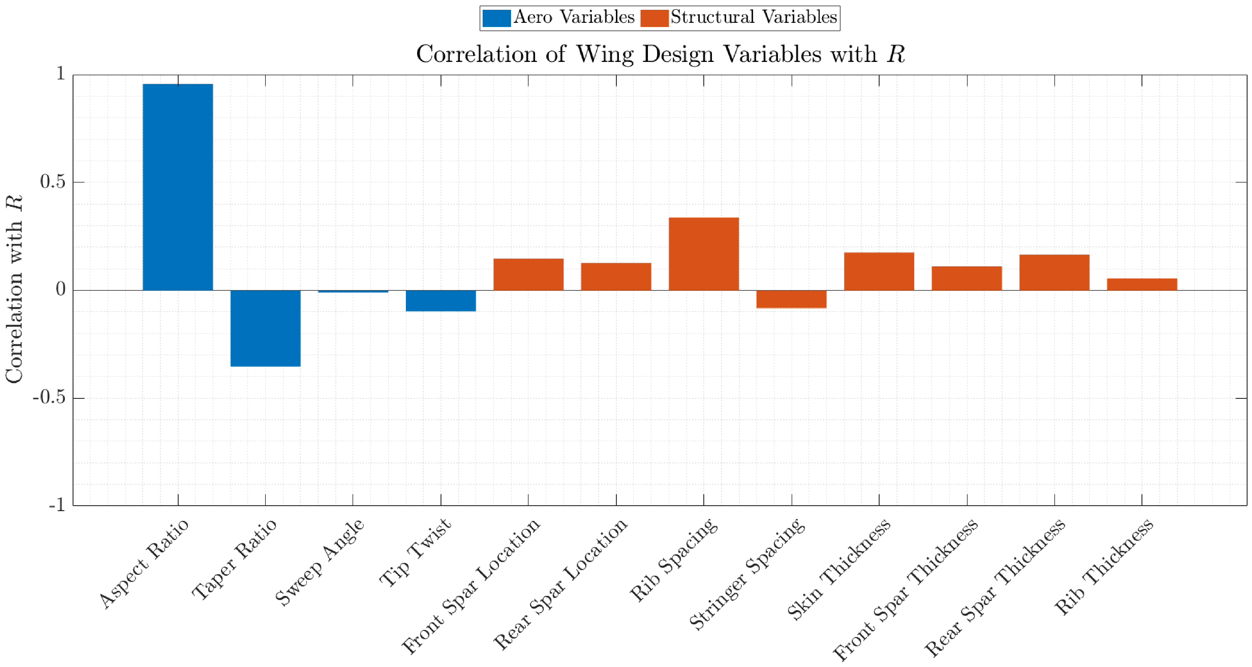
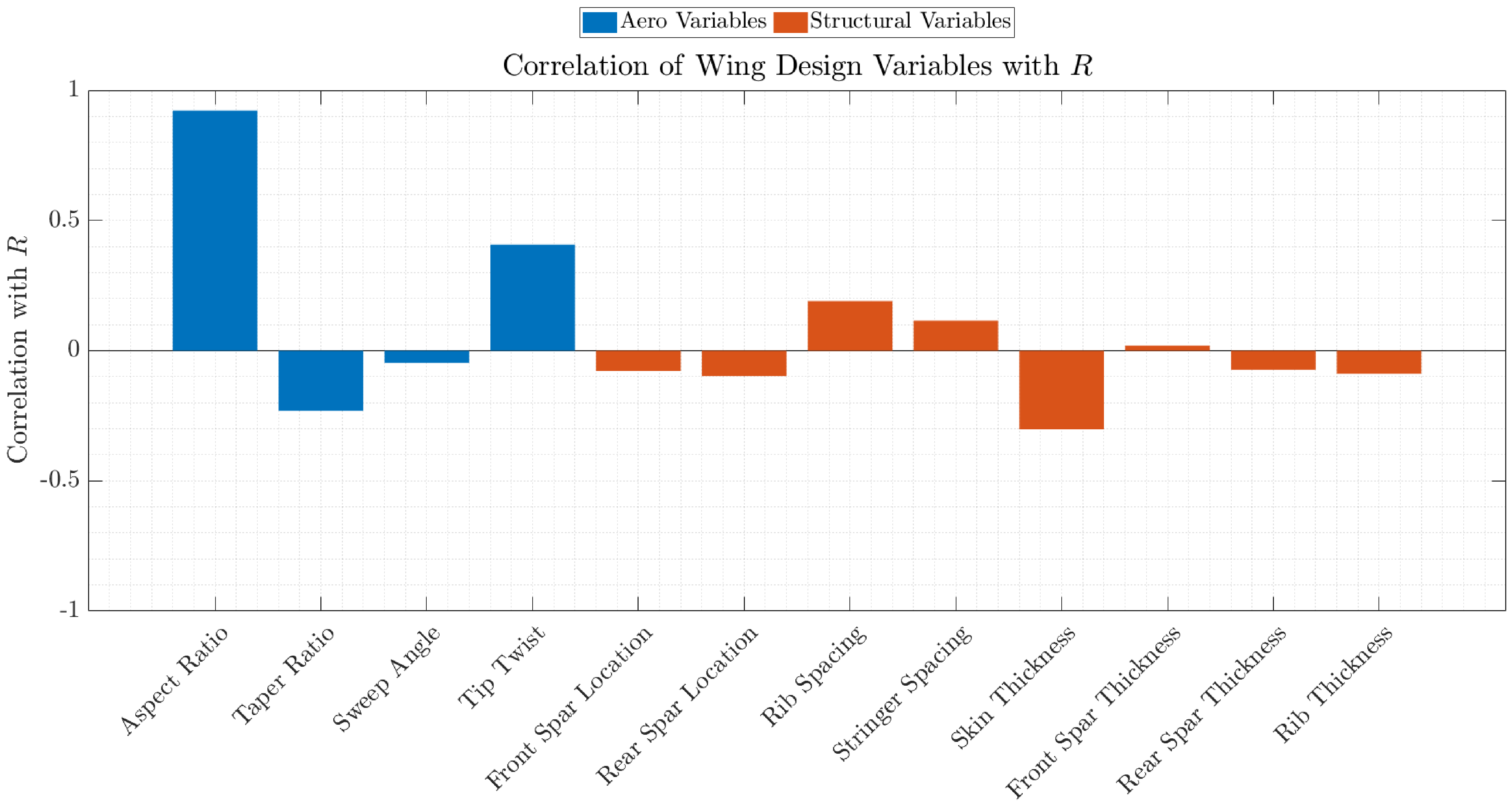
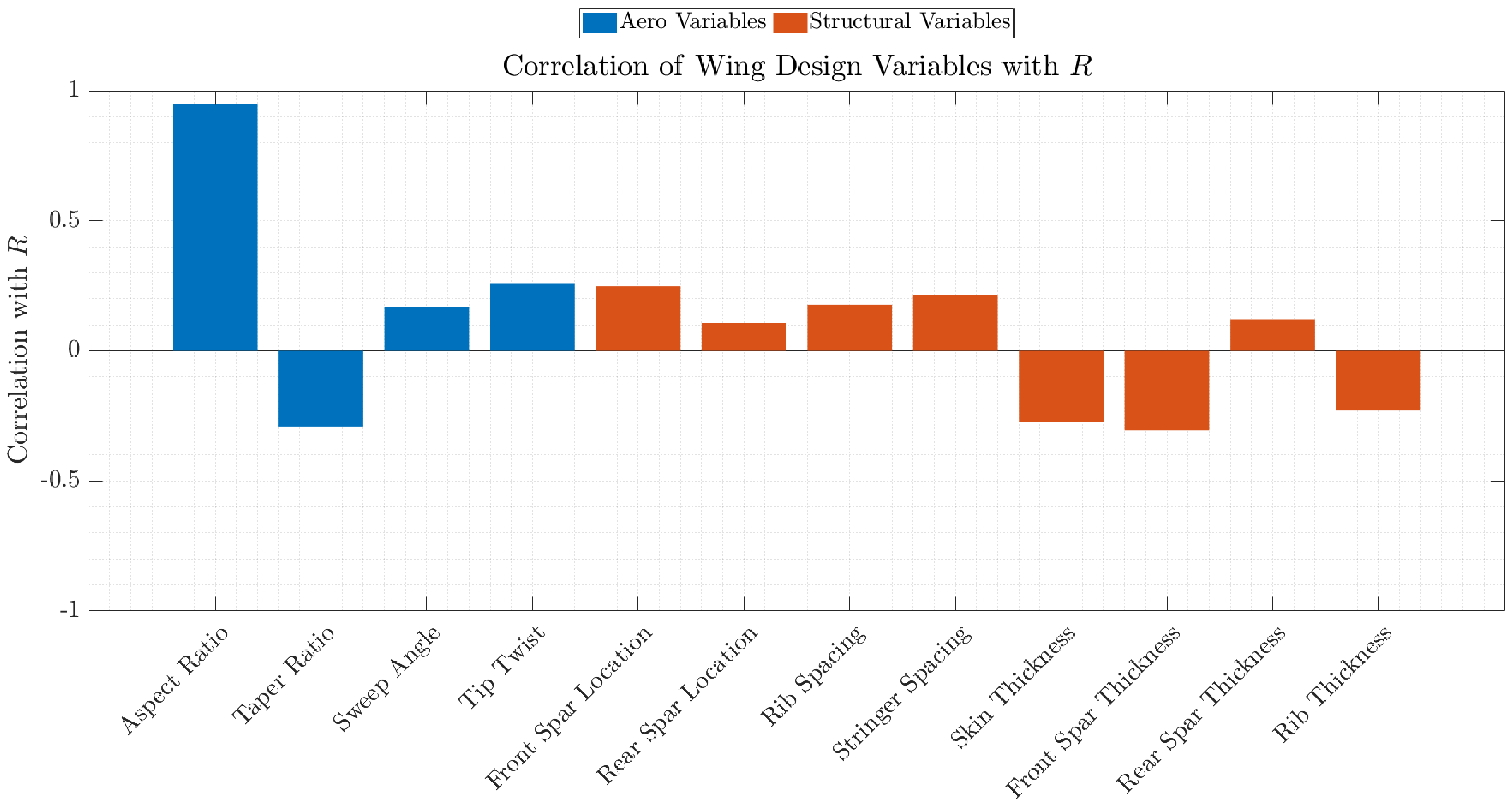
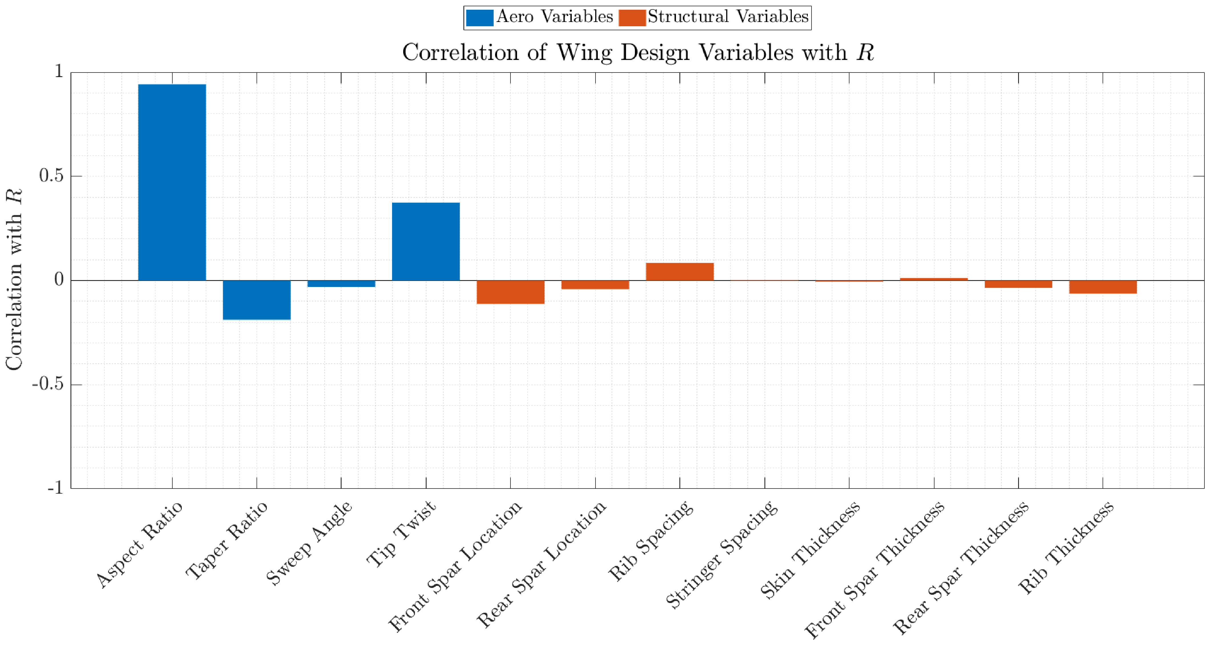
Figure 13 presents the correlation between wing design variables and range R for the fifth and final iteration, reflecting the fully converged design space. Consistent with all previous iterations (Figure A2, Figure A6, Figure A10 and Figure A14), the aspect ratio remains the dominant driver of range, exhibiting a very strong positive correlation (≃0.94). The tip twist also maintains a moderate positive correlation (≃0.43), reinforcing its role as the most influential secondary aerodynamic variable. In contrast, the taper ratio continues to show a moderate negative correlation (≃−0.30), while the sweep angle retains only a weak negative influence, confirming its limited impact on range. The influence of structural variables becomes more clearly defined but remains relatively secondary compared to aerodynamic parameters. Stringer spacing shows a small positive correlation, while rib spacing and front spar location exhibit only weak positive effects. On the other hand, several structural variables display consistent negative correlations with range, most notably rear spar location (≃−0.22), skin thickness (≃−0.27), rear spar thickness (≃−0.10), and rib thickness (≃−0.14). These trends suggest that increases in structural thickness and certain placement parameters tend to reduce range, likely due to associated weight penalties. Overall, the final iteration confirms a stable and well-defined relationship structure: aerodynamic variables—particularly aspect ratio and tip twist—dominate range performance, while structural variables exert smaller, mostly negative influences. This indicates that, at convergence, the optimization has clearly identified the primary performance drivers and reduced uncertainty in the role of secondary design variables.
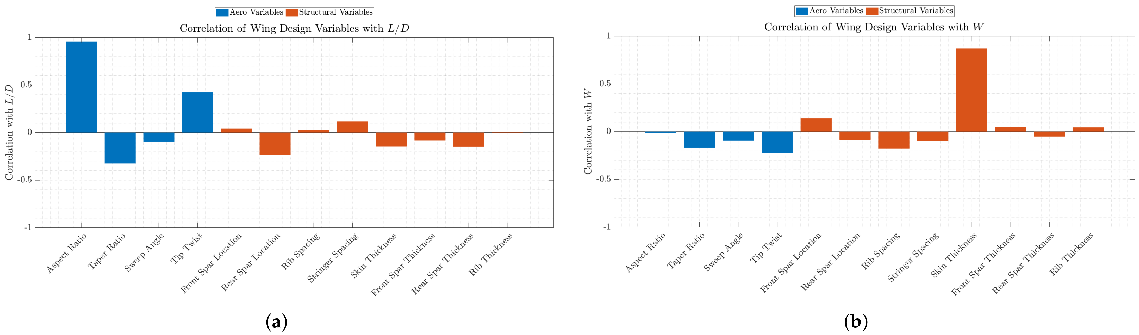
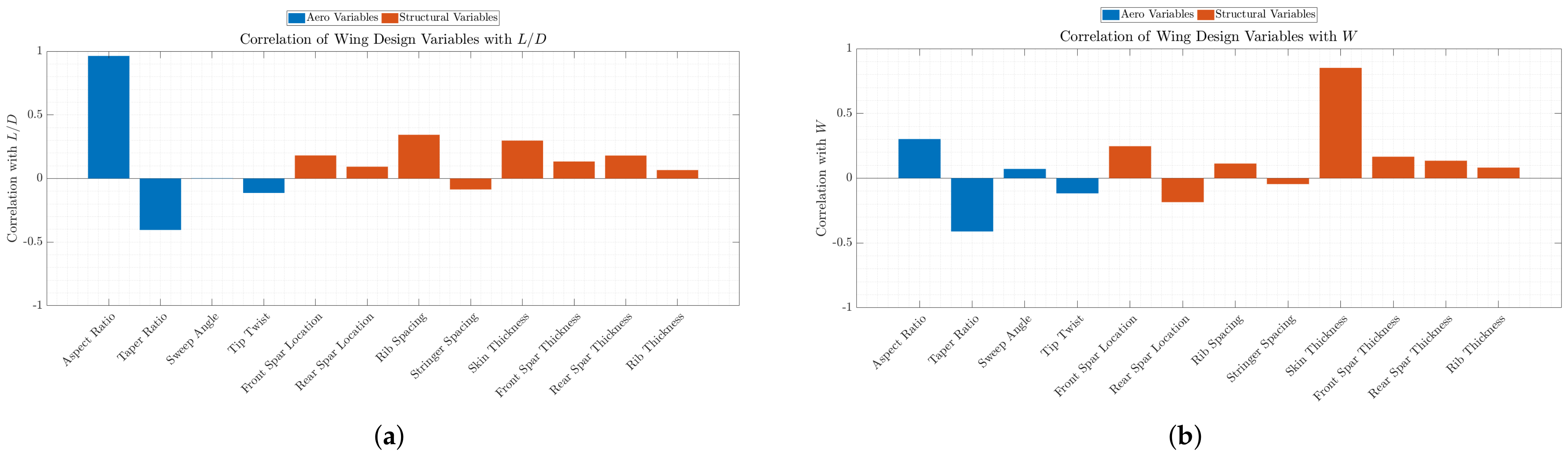
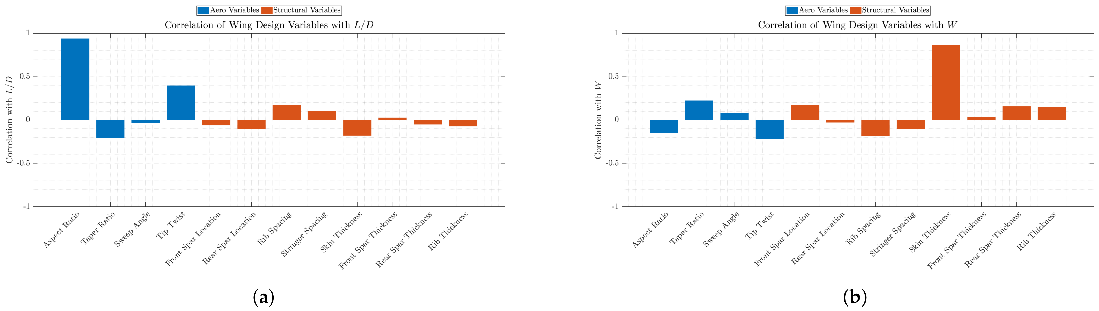
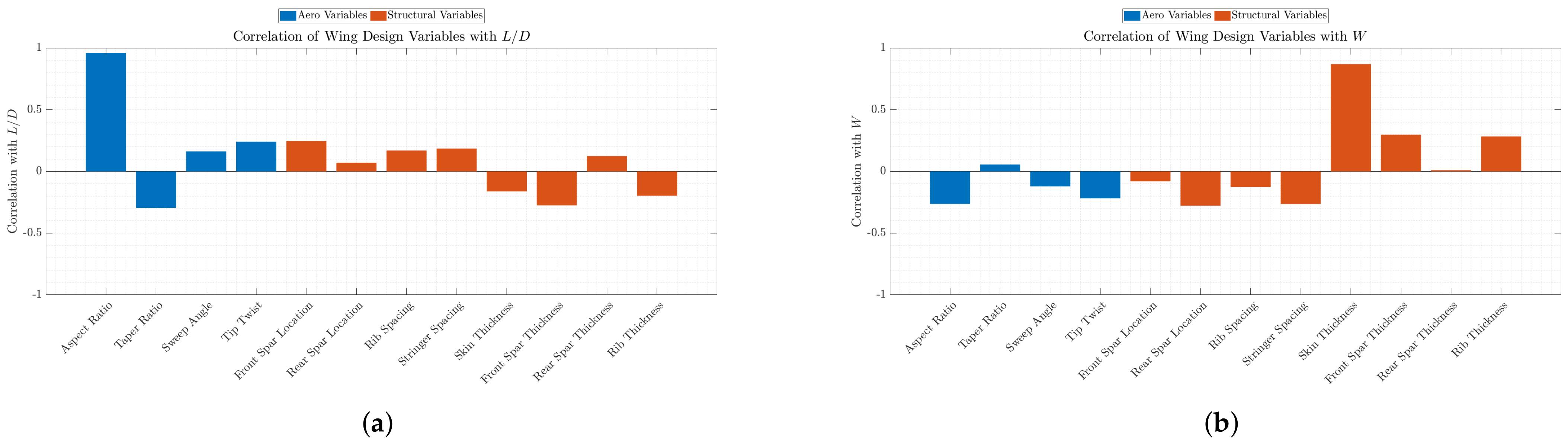
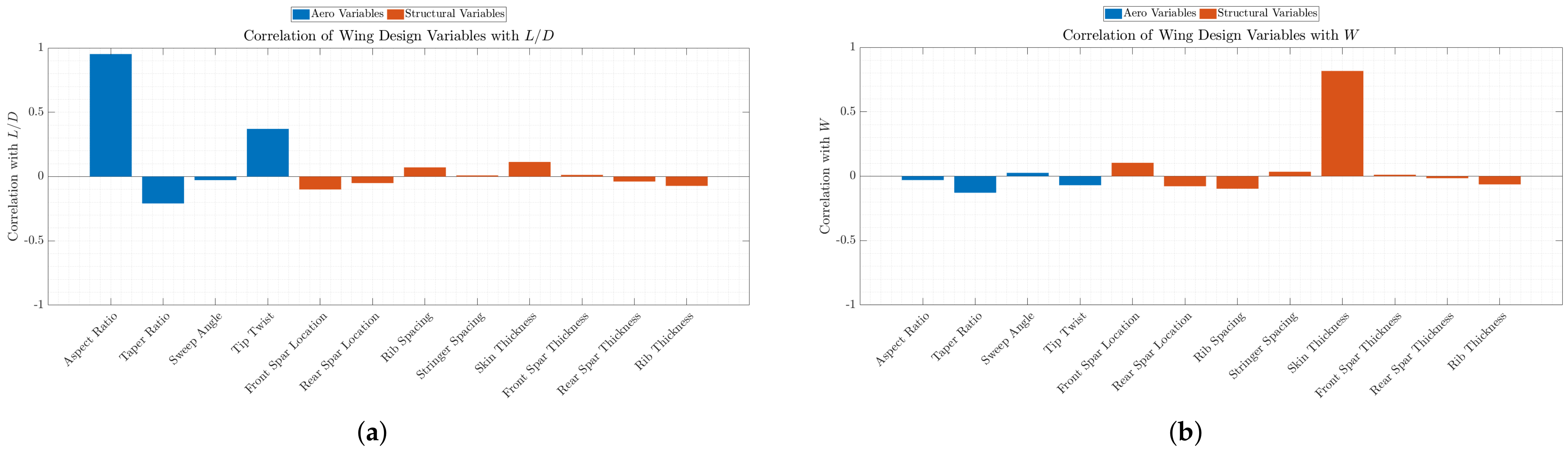
Figure 14 shows the correlation of aerodynamic and structural design variables with L/D(a) and weight W(b) for the fifth SBO iteration, reflecting the fully converged relationships in the design space. For L/D (Figure 14a), the aspect ratio remains the dominant parameter, exhibiting a consistently strong positive correlation (≃0.95). The tip twist retains a moderate positive correlation (≃0.4), confirming its role as the most influential secondary aerodynamic variable. The taper ratio continues to show a moderate negative correlation, while the sweep angle has only a weak negative effect. Compared to earlier iterations, the influence of structural variables on L/D is minimal. Most structural parameters cluster close to zero, with only small negative correlations observed for rear spar location, skin thickness, and spar thicknesses, indicating a weak detrimental effect on aerodynamic efficiency. For weight W (Figure 14b), structural variables clearly dominate. Skin thickness maintains a very strong positive correlation (≃0.85), confirming it as the primary driver of weight. Other structural variables, such as front spar location, rib spacing, and stringer spacing, show small negative correlations, while spar thicknesses and rib thickness exhibit weak positive or near-zero effects. Aerodynamic variables have negligible influence on weight, with correlations remaining close to zero or weakly negative. Overall, the final iteration demonstrates a well-converged and decoupled relationship structure, where L/D is governed almost entirely by aerodynamic variables (primarily aspect ratio and tip twist), and weight is dominated by structural thickness—especially skin thickness—with minimal cross-coupling between aerodynamic and structural design variables.
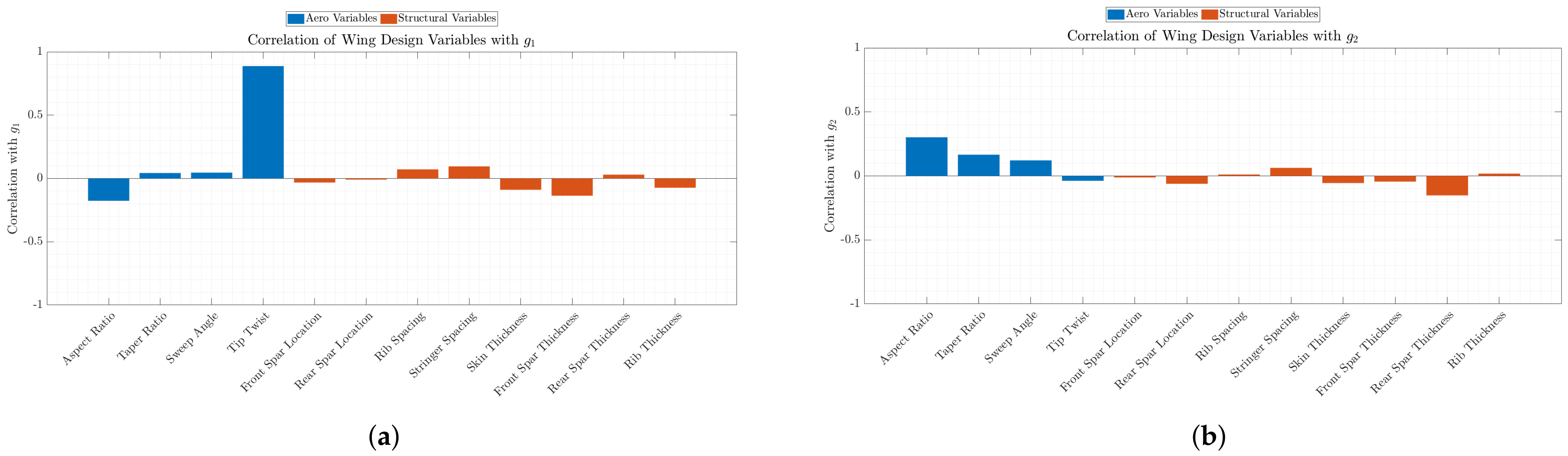
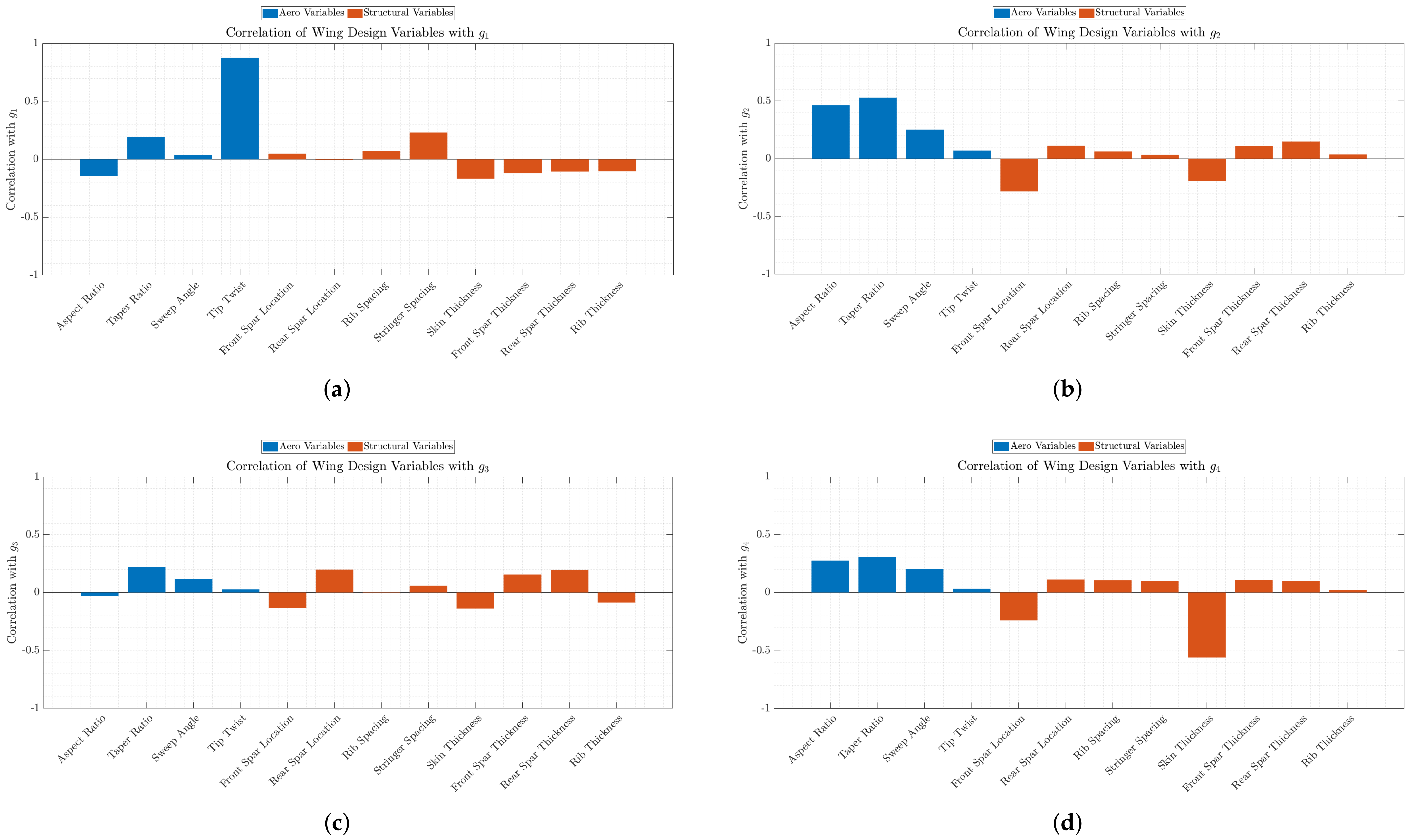
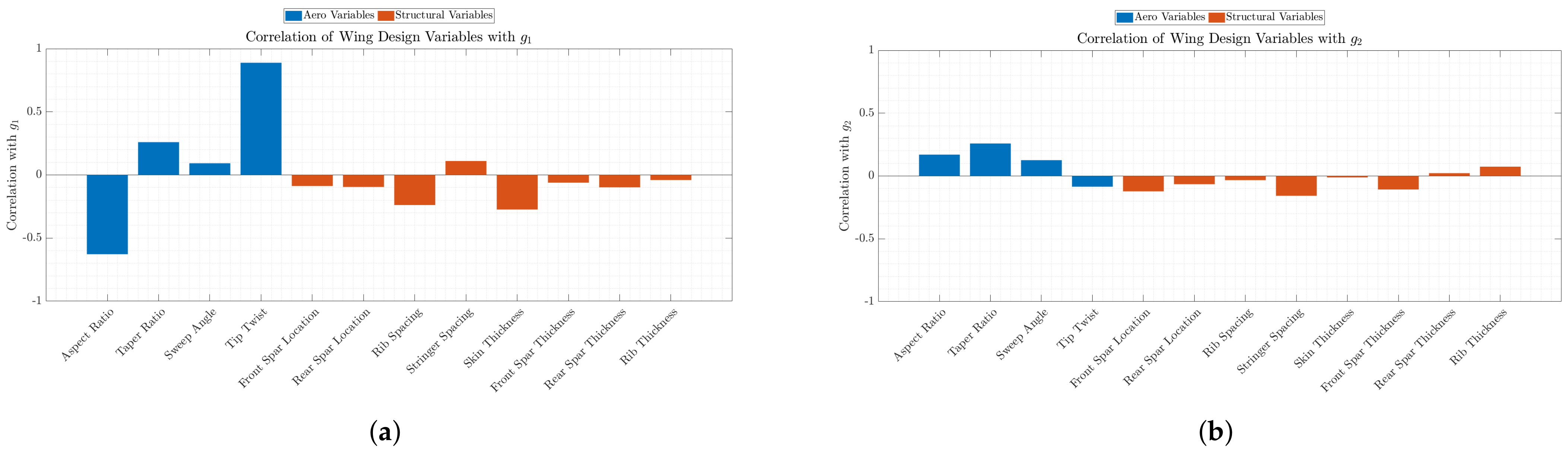
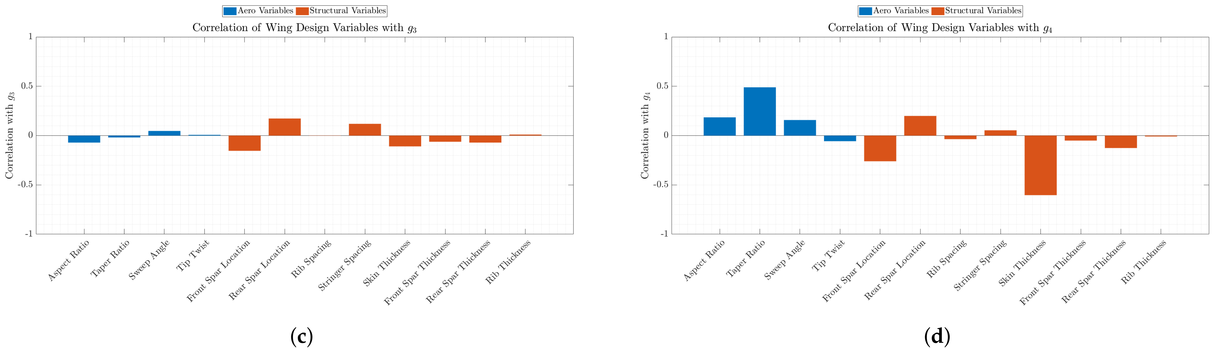
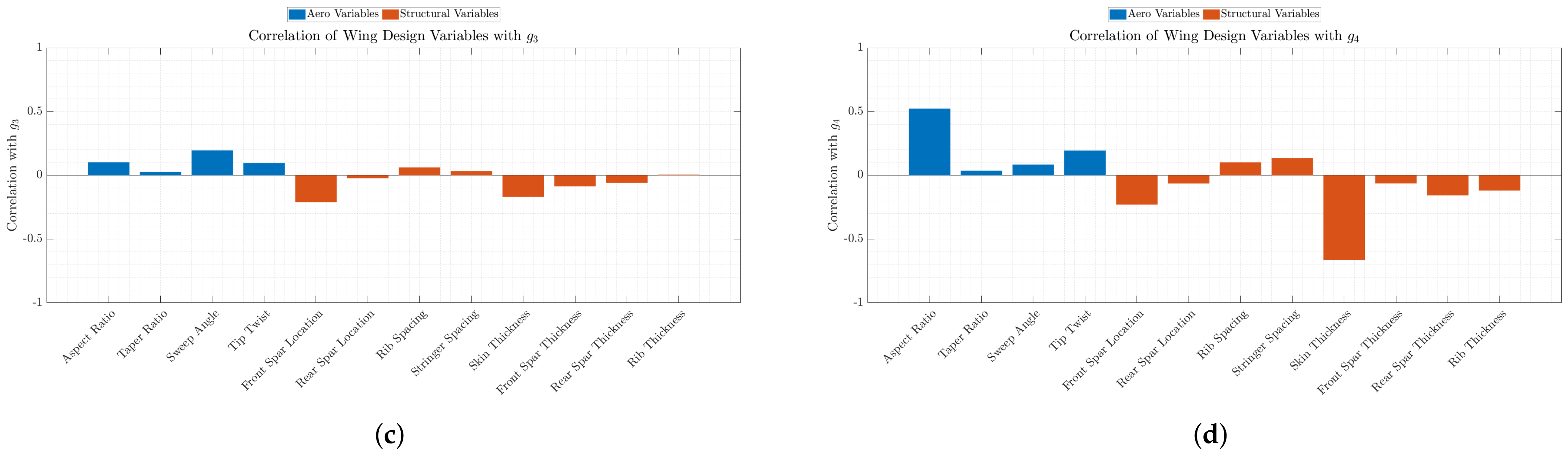
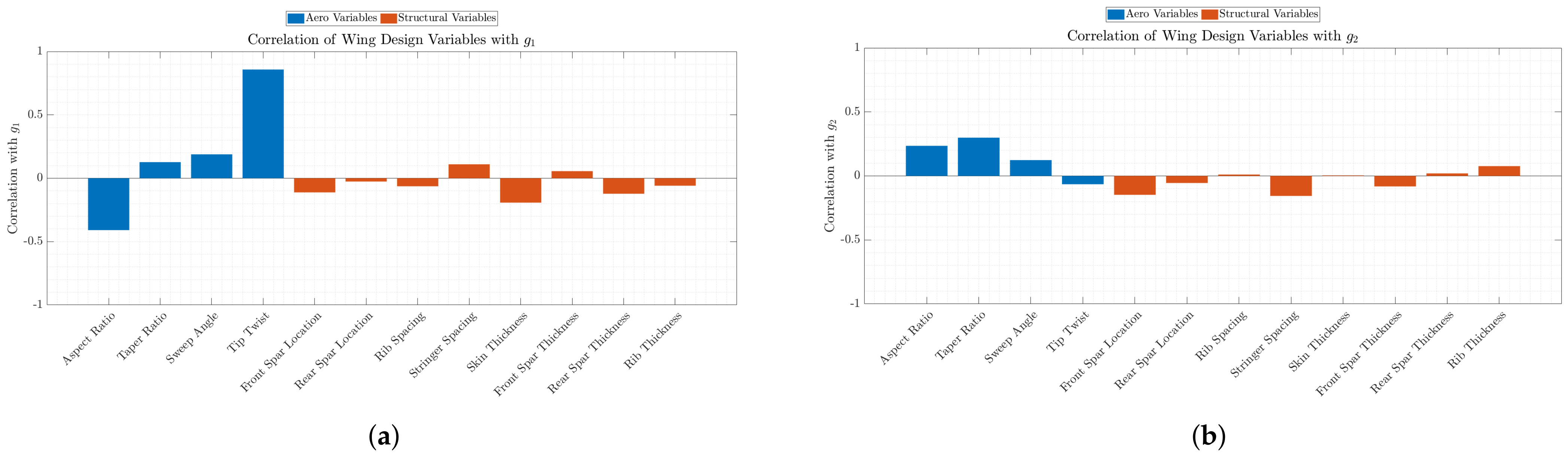
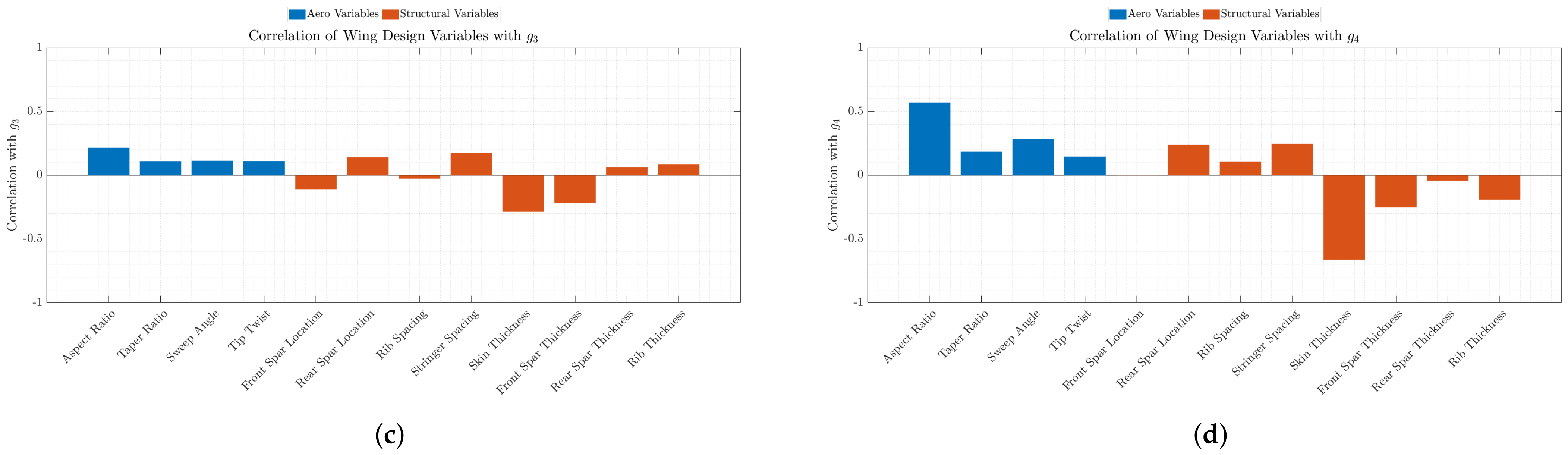
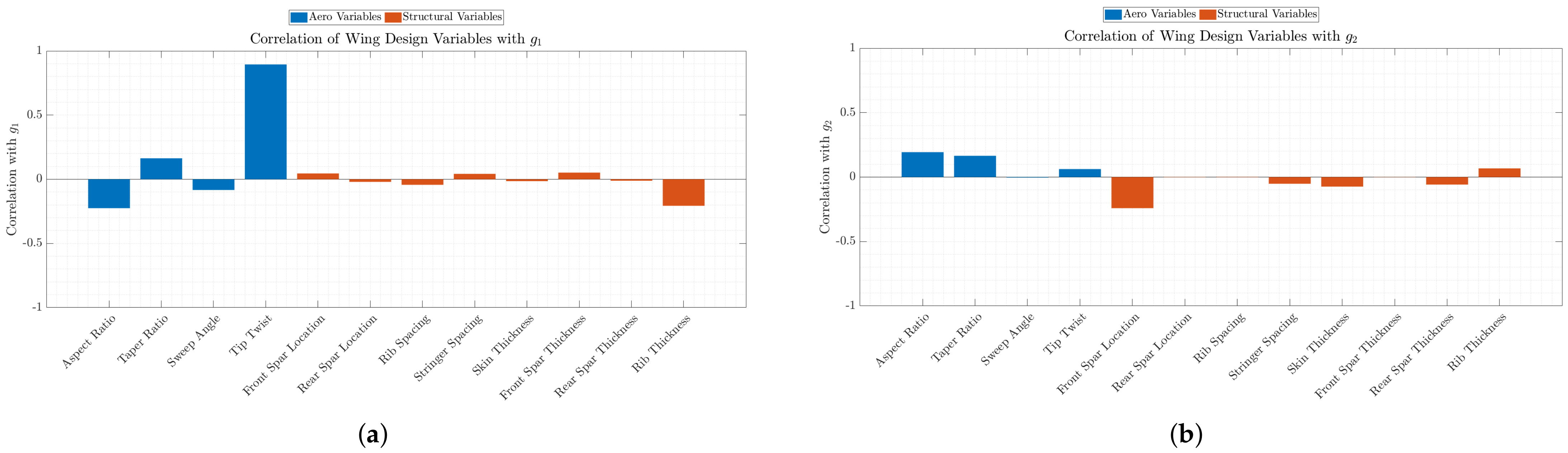
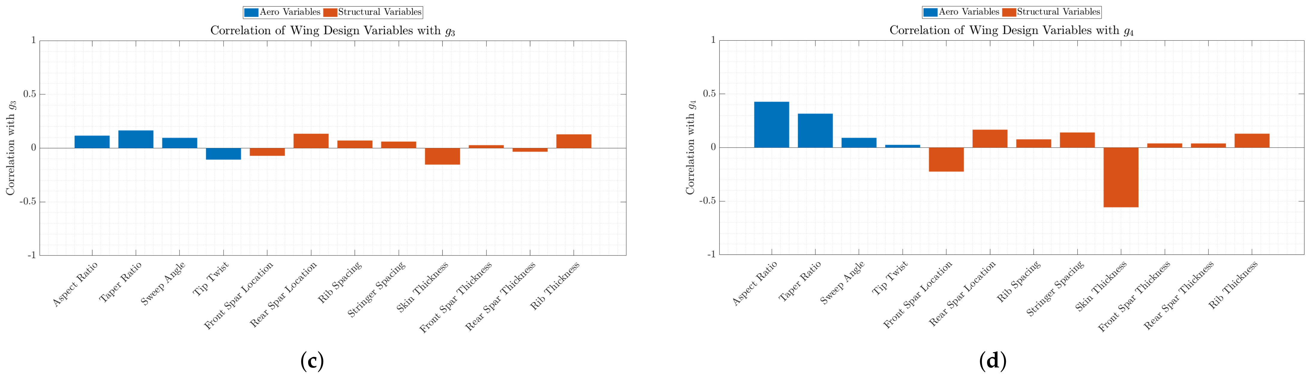
Figure 15 presents the correlation of aerodynamic and structural design variables with the constraint functions g 1 , g 2 , g 3 and g 4 for the fifth SBO iteration, reflecting the fully converged constraint–design relationships. As in previous iterations (Figure A4, Figure A8, Figure A12 and Figure A16), all constraints are defined such that g i < 0 corresponds to feasible designs; thus, negative correlations indicate improved constraint satisfaction, while positive correlations indicate a tendency toward violation.
For g 1 (Figure 15a), tip twist remains the dominant variable, exhibiting a strong positive correlation, confirming that increasing twist drives the design toward violating this constraint. Aspect ratio shows a weak negative correlation, indicating a slight improvement in feasibility with increasing aspect ratio. Structural variables exhibit minimal influence, with only very small correlations, suggesting that g 1 is primarily governed by aerodynamic variables at convergence.
For g 2 (Figure 15b), a clearer aerodynamic influence emerges. Aspect ratio, taper ratio, and sweep angle show moderate positive correlations, indicating that increasing these parameters tends to reduce feasibility. In contrast, structural variables show mixed but generally weak effects, with front spar location exhibiting a noticeable negative correlation, suggesting a potential role in improving constraint satisfaction.
For g 3 (Figure 15c), the correlations remain relatively weak overall. Aerodynamic variables show small positive correlations, while structural variables display mixed behavior. Rear spar location and front spar thickness show positive correlations, whereas skin thickness and rib thickness show negative correlations, indicating that increasing structural thickness helps satisfy this constraint.
For g 4 (Figure 15d), the strongest and most consistent relationships are observed. Aerodynamic variables—particularly aspect ratio, taper ratio, and sweep angle—show moderate positive correlations, indicating that improvements in aerodynamic performance tend to push the design toward constraint violation. In contrast, skin thickness exhibits a strong negative correlation, with additional negative contributions from spar thicknesses and rib thickness, confirming that structural sizing remains the primary mechanism for restoring feasibility.
Overall, the final iteration demonstrates a well-defined and decoupled constraint structure: g 1 and g 2 are primarily influenced by aerodynamic variables, g 3 shows weak and mixed sensitivity, and g 4 remains the most critical constraint, governed by a balance between aerodynamic drivers (causing violation) and structural thickness variables (ensuring feasibility).
Table 8 and Table 9 show the feasible designs of the 5th SBO iteration, for both samples and infills, respectively. Constraints g 1 and g 4 remain close to zero for the feasible configurations, indicating that they primarily govern the optimal solutions. In contrast, g 2 and g 3 exhibit significantly negative values across all configurations, suggesting that they are inactive and do not restrict the optimization. The most feasible designs are characterized by by high lift-to-drag ratio values and a relatively narrow range of weight, confirming that improvements in aerodynamic efficiency drive the range optimization. The infill results further demonstrate convergence towards a well-defined region of the design space. Overall, this indicates that the optimization successfully identifies feasible, high-performance configurations, where the trade-off between maximizing range and satisfying the most critical constraints— g 1 and g 4 —defines the optimal design boundaries.

Aerostructural Analysis of the Best Configuration

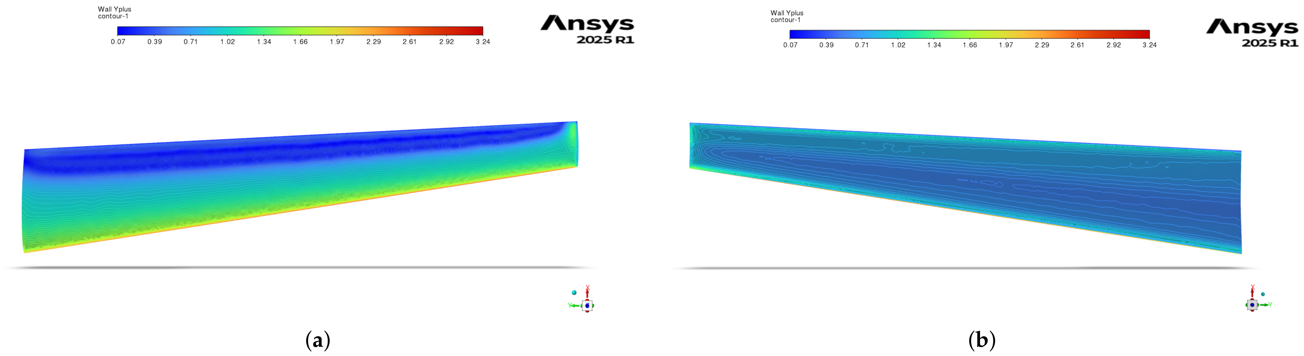
This subsection presents the aerodynamic analysis results obtained at an angle of attack of 12 , which were used as the basis for the FEM analyses. Figure 16 illustrates the contours of the Y + distribution over the upper and lower surfaces of the selected wing configuration, where the values range from 0 to 3.24.
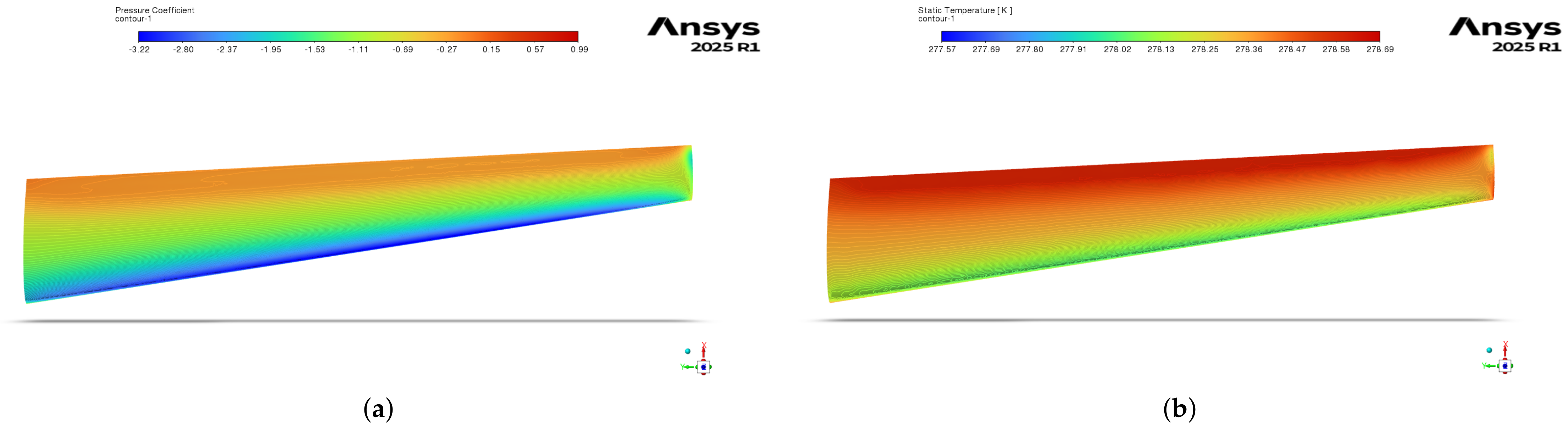
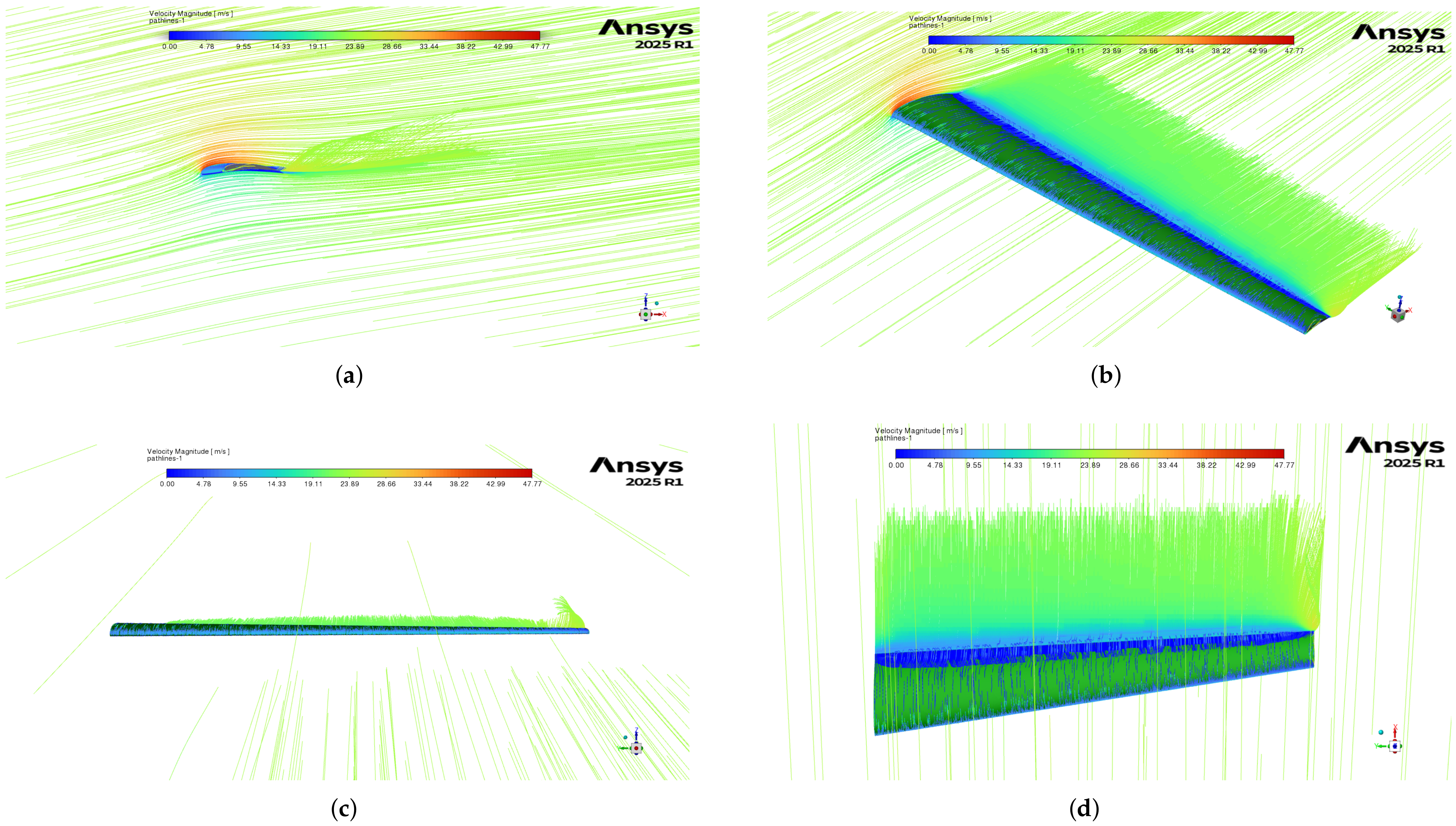
Figure 17 presents the pressure coefficient and temperature contours on the upper wing surface obtained from the aerodynamic analysis at 12 AoA. A minor flow separation is observed near the trailing edge, along with a small vortex forming at the wing tip.
The previously discussed flow detachment is more clearly demonstrated in Figure 18, which presents the airflow pathlines for the examined case. In Figure 18b,d, a small vortex forms near the trailing edge, characterized by flow rotation about the y-axis, resulting in localized flow separation. Additionally, Figure 18c provides a clearer view of the tip vortex.
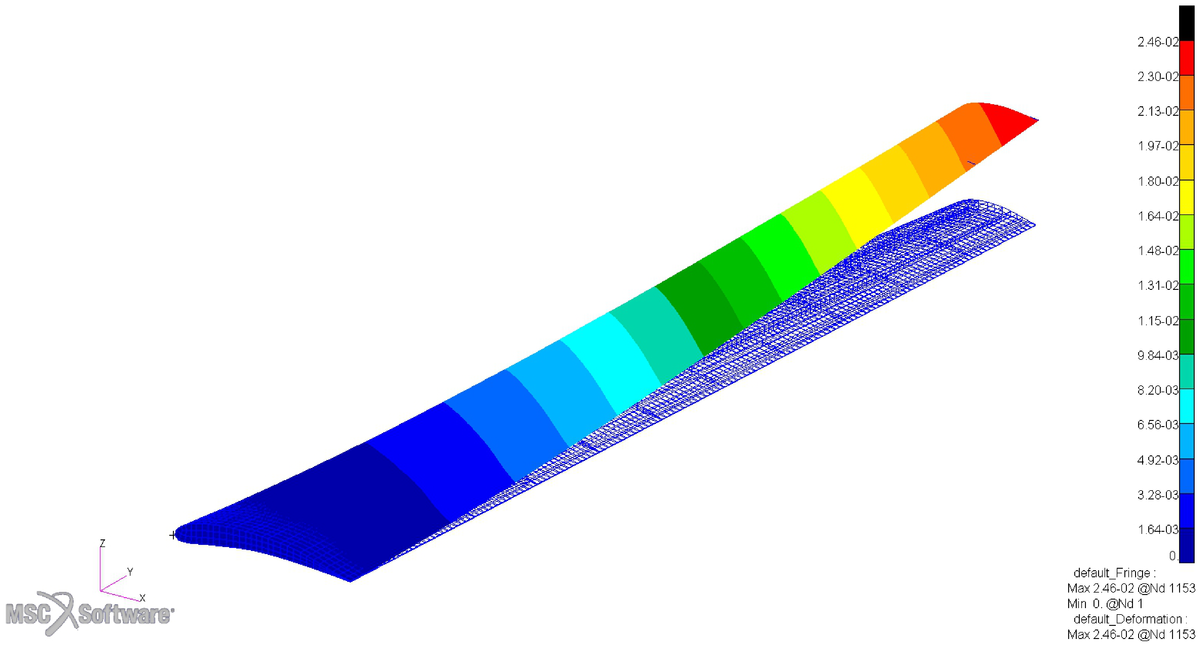
The structural response of the optimal wing configuration is also examined, providing important insight in the structural behavior of the optimized design and confirming the effectiveness of the proposed aerostructural optimization framework. In particular, Figure 19 illustrates the displacement field of the wing under aerodynamic loading. The deformation pattern is dominated by bending, with maximum deflection occurring at the wing tip, which is consistent with typical cantilever wing behavior. The magnitude of deformation remains within acceptable limits, ensuring that aerodynamic performance is not significantly degraded due to excessive aeroelastic effects. This result further demonstrates that the optimized design achieves a suitable compromise between structural flexibility and stiffness.
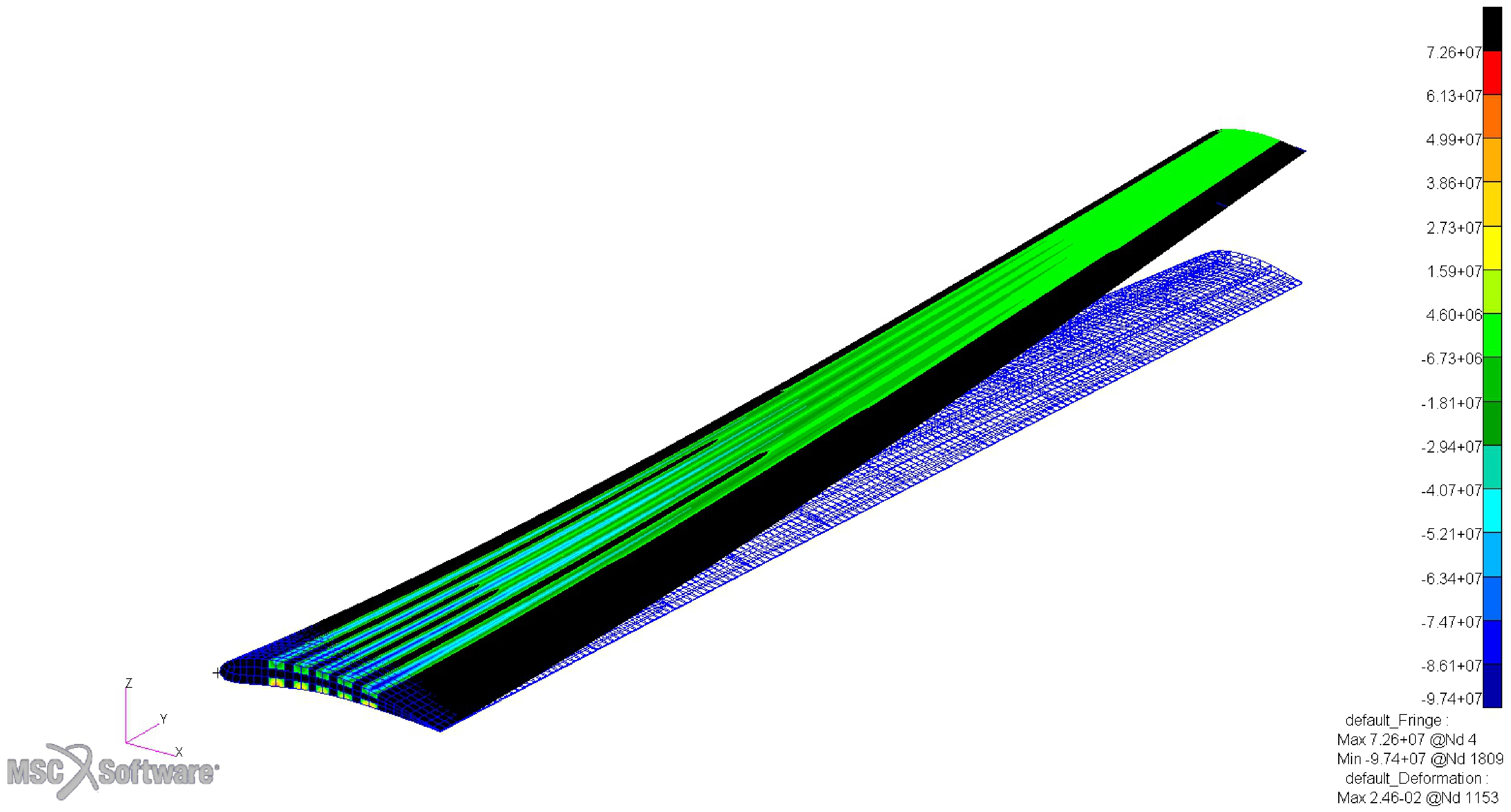
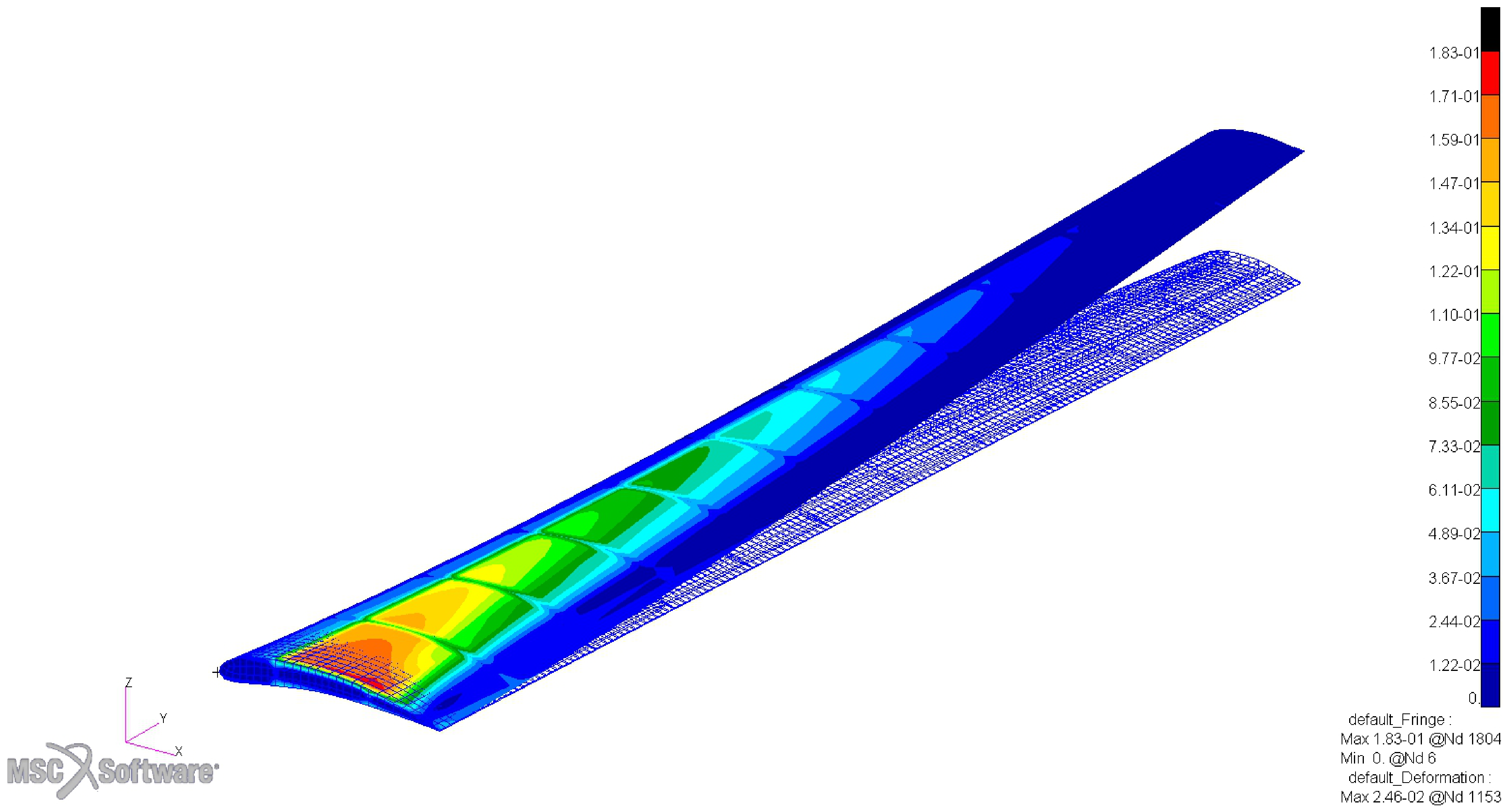
The distribution of the maximum failure index across the wing structure is also presented in Figure 20. The highest values are observed near the wing root region, where bending moments are largest due to aerodynamic loading. Despite these localized peaks, the maximum failure index remains below the allowable limit, confirming that the optimized structure satisfies the strength constraints. A similar trend is observed for the maximum beam stress distribution within the structural members (Figure 21). Elevated stress levels are again concentrated near the wing root and along primary load-carrying components such as spars, reflecting the load transfer mechanism within the wing. The stress distribution is smooth and does not exhibit abrupt concentrations, suggesting that the structural layout and sizing variables have been appropriately tuned during the optimization process. The absence of excessive stress peaks further confirms that the design achieves an efficient balance between weight minimization and structural integrity. Overall, the structural response of the optimal configuration demonstrates that the proposed SBO framework successfully captures the interaction between aerodynamic loading and structural behavior. The results confirm that structural variables, particularly skin thickness and internal layout parameters, are actively driven by strength and stability constraints, while aerodynamic variables govern performance. This interplay leads to a structurally efficient and aerodynamically optimized wing design.


4. Discussion and Conclusions

This study presented an aerostructural optimization framework for the preliminary design of a low-Reynolds-number composite UAV wing, integrating CFD and FEM analyses within a surrogate-based optimization (SBO) approach. The methodology enabled efficient exploration of a multidisciplinary design space, combining aerodynamic planform variables with structural sizing parameters, while significantly reducing the computational cost associated with repeated high-fidelity model evaluations.
The results demonstrated that the proposed SBO framework is capable of consistently converging toward feasible high-performance solutions across multiple independent optimization runs. The surrogate models exhibited strong predictive capability, as confirmed by RMSE and Leave-One-Out validation metrics, indicating reliable approximation of the underlying model responses throughout the optimization process.
From a design perspective, the results reveal a clear separation of roles among the design variables. Aerodynamic parameters, particularly aspect ratio and tip twist, were identified as the primary drivers of range performance due to their direct influence on lift-to-drag ratio. In contrast, structural variables—most notably skin thickness—played a critical role in satisfying strength and buckling constraints, thereby defining the feasible design space. The optimal solutions emerged from the interaction between performance-driven aerodynamic variables and constraint-driven structural sizing, highlighting the importance of accounting for aerostructural interactions even in preliminary design stages.
The optimal wing configuration achieved a maximum range of approximately 203 km while satisfying all aerodynamic and structural constraints, demonstrating the effectiveness of the proposed framework for early-stage UAV design. Furthermore, the consistency of the results across different Design of Experiments (DoE) strategies indicates robustness with respect to initial sampling, reinforcing the reliability of the SBO approach.
Despite these promising results, several limitations remain. The present study relies on steady RANS simulations and linear structural analysis, which do not capture transition effects, unsteady aerodynamic phenomena, or geometric nonlinearities in highly flexible wings. While these effects may influence the detailed aerodynamic and structural response, the adopted modeling approach is considered appropriate for preliminary design, where the objective is to capture the dominant trends governing performance and constraints while maintaining computational tractability within the surrogate-based optimization framework. This modeling level is consistent with common practice in early-stage aerostructural optimization studies.
Future work will focus on extending the proposed framework to address these limitations. In particular, the incorporation of geometrically nonlinear structural models and unsteady aerodynamic simulations would enable more accurate prediction of aeroelastic behavior. The integration of uncertainty quantification and reliability-based design optimization (RBDO) techniques represents another important direction, allowing for more robust and realistic design solutions. Furthermore, the application of multi-fidelity strategies could further improve computational efficiency by combining low- and high-fidelity models within the SBO framework. A limitation of the present structural modeling approach is the use of equivalent isotropic properties for beam elements, which does not capture anisotropic coupling effects of composite laminates, such as bend–twist coupling. These effects can be exploited in composite wings for passive load alleviation and improved aeroelastic performance. Their inclusion would require higher-fidelity laminate modeling and additional design variables (e.g., stacking sequence), increasing the complexity and computational cost of the optimization problem. Furthermore, preliminary aeroelastic analyses suggest a limited impact of structural deformation on aerodynamic performance for the examined configurations. However, this effect may become more significant for highly flexible designs and should be addressed through fully coupled aeroelastic analysis in future work. Finally, the extension of the methodology to full aircraft configurations, including fuselage and tail interactions, would provide a more comprehensive assessment of overall aircraft performance. Overall, the proposed aerostructural SBO framework provides a robust and efficient tool for the preliminary design of low-Reynolds-number UAV wings, bridging the gap between physics-based analysis and computationally tractable optimization.

Author Contributions

Conceptualization, E.N. and S.K.; methodology, E.N. and S.K.; software, E.N., S.K. and P.K.; validation, E.N., S.K. and P.K.; formal analysis, E.N. and S.K.; investigation, E.N. and S.K.; resources, E.N., S.K. and P.K.; data curation, E.N., S.K. and P.K.; writing—original draft preparation, E.N. and S.K.; writing—review and editing, E.N. and S.K.; visualization, E.N. and S.K.; supervision, S.K., P.K., V.L. and V.K.; project administration, E.N., S.K., V.L. and V.K. All authors have read and agreed to the published version of the manuscript.

Funding

This research received no external funding.

Data Availability Statement

Data are available on request.

Conflicts of Interest

The authors declare no conflicts of interest.

Abbreviations

The following abbreviations are used in this manuscript:
AoAAngle of Attack
ASLAbove Sea Level
CFDComputational Fluid Dynamics
DoEDesign of Experiments
DoFDegrees of Freedom
EIExpected Improvement
FEMFinite Element Method
FVMFinite Volume Method
LHSLatin Hypercube Sampling
LOOLeave-One-Out
MACMean Aerodynamic Chord
MSEMean Square Error
RANSReynolds-Averaged Navier–Stokes
RMSERoot Mean Square Error
SBOSurrogate-Based Optimization
SLSea Level
UAVUnmanned Aerial Vehicle

Appendix A. SBO Additional Iterations

Appendix A.1. 1st Iteration

Figure A1. First SBO iter.—correlation between objective and constraints.
Drones 10 00352 g0a1
Figure A2. First SBO iter.—correlation of aerodynamic and structural design parameters with Range-Objective.
Drones 10 00352 g0a2
Figure A3. First SBO iter.—correlation of aerodynamic and structural design parameters with L / D (a), and W e i g h t (b).
Drones 10 00352 g0a3
Figure A4. First SBO iter.—correlation of aerodynamic and structural design parameters with g 1 (a), g 2 (b), g 3 (c), and g 4 (d).
Drones 10 00352 g0a4aDrones 10 00352 g0a4b

Appendix A.2. 2nd DoE

Figure A5. Second SBO iter.—correlation between objective and constraints.
Drones 10 00352 g0a5
Figure A6. Second SBO iter.—correlation of aerodynamic and structural design parameters with Range-Objective.
Drones 10 00352 g0a6
Figure A7. Second SBO iter.—correlation of aerodynamic and structural design parameters with L / D (a), and W e i g h t (b).
Drones 10 00352 g0a7
Figure A8. Second SBO iter.—correlation of aerodynamic and structural design parameters with g 1 (a), g 2 (b), g 3 (c), and g 4 (d).
Drones 10 00352 g0a8aDrones 10 00352 g0a8b

Appendix A.3. 3rd DoE

Figure A9. Third SBO iter.—correlation between objective and constraints.
Drones 10 00352 g0a9
Figure A10. Third SBO iter.—correlation of aerodynamic and structural design parameters with Range-Objective.
Drones 10 00352 g0a10
Figure A11. Third SBO iter.—correlation of aerodynamic and structural design parameters with L / D (a), and W e i g h t (b).
Drones 10 00352 g0a11
Figure A12. Third SBO iter–Correlation of aerodynamic and structural design parameters with g 1 (a), g 2 (b), g 3 (c), and g 4 (d).
Drones 10 00352 g0a12aDrones 10 00352 g0a12b

Appendix A.4. 4th DoE

Figure A13. Fourth SBO iter.—correlation between objective and constraints.
Drones 10 00352 g0a13
Figure A14. Fourth SBO iter.—correlation of aerodynamic and structural design parameters with Range-Objective.
Drones 10 00352 g0a14
Figure A15. Fourth SBO iter.—correlation of aerodynamic and structural design parameters with L / D (a), and W e i g h t (b).
Drones 10 00352 g0a15
Figure A16. Fourth SBO iter.—correlation of aerodynamic and structural design parameters with g 1 (a), g 2 (b), g 3 (c), and g 4 (d).
Drones 10 00352 g0a16aDrones 10 00352 g0a16b

Appendix A.5. CFD Validation and Verification Study

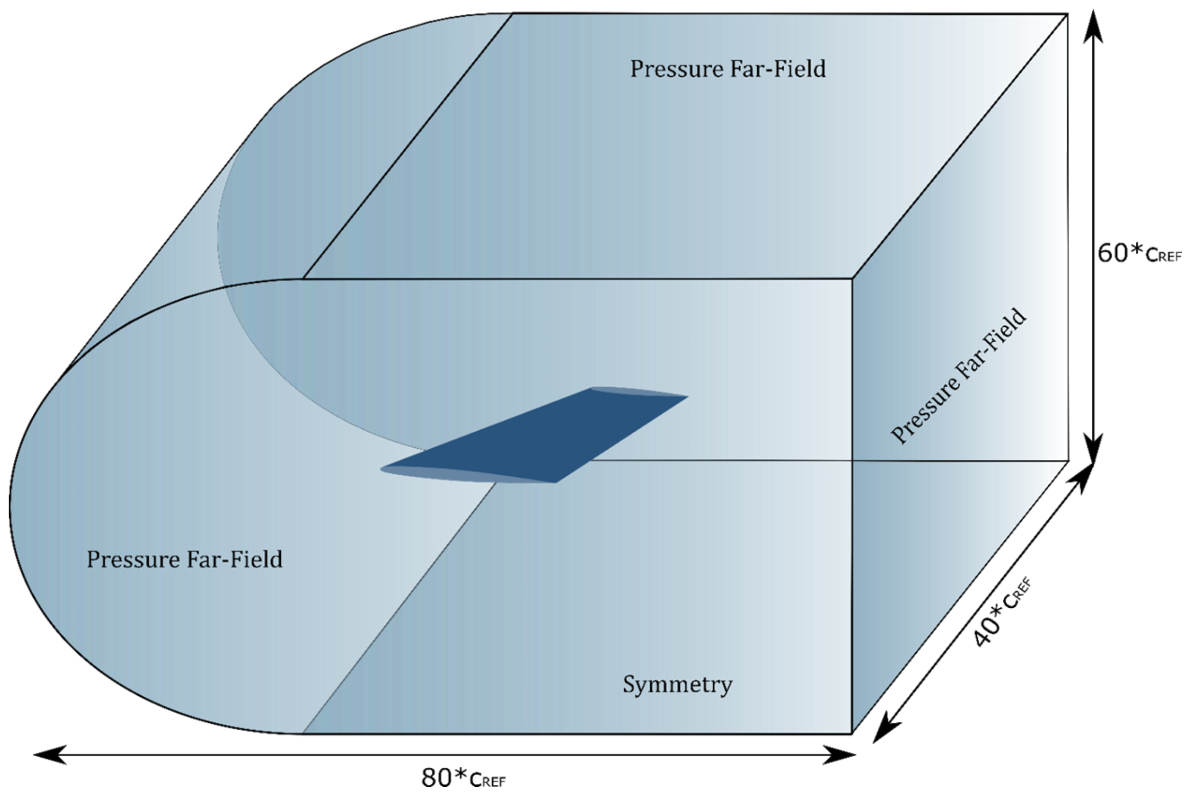
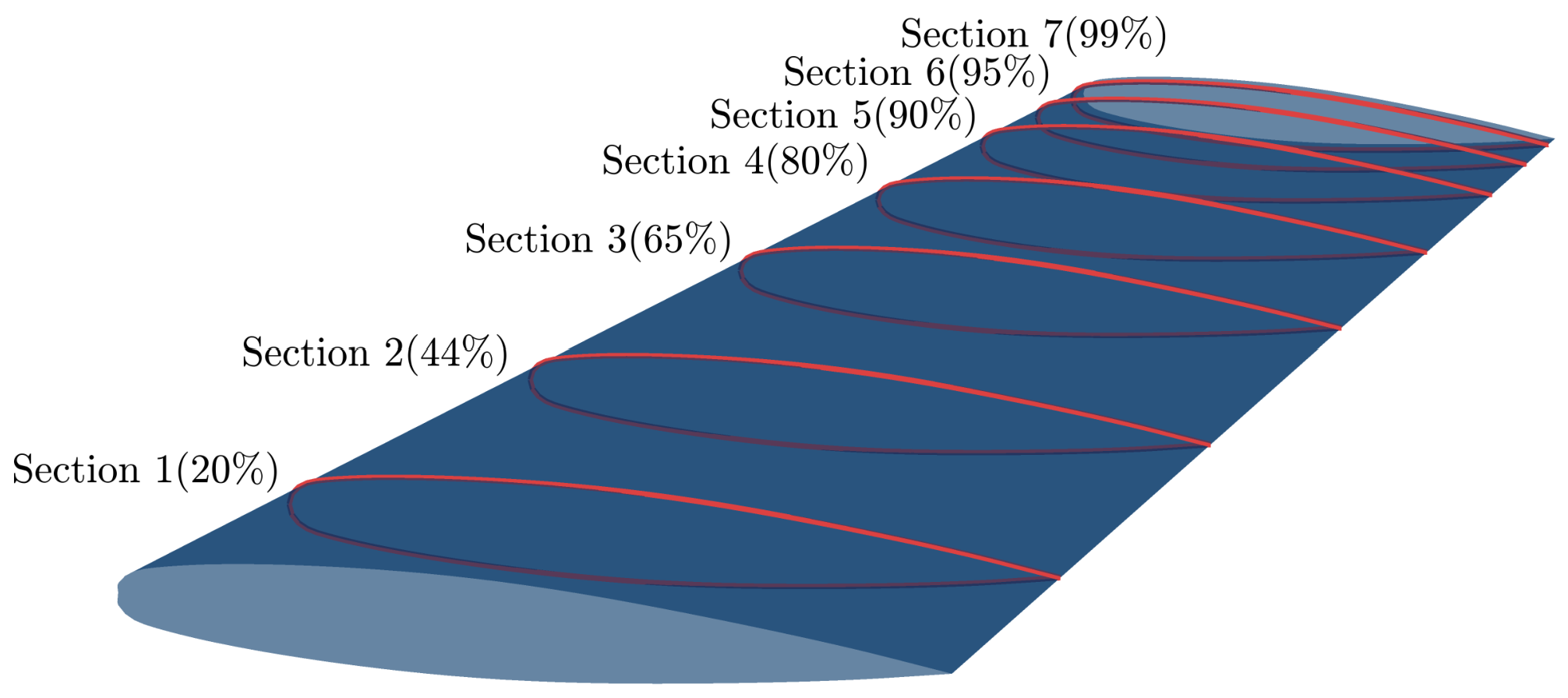
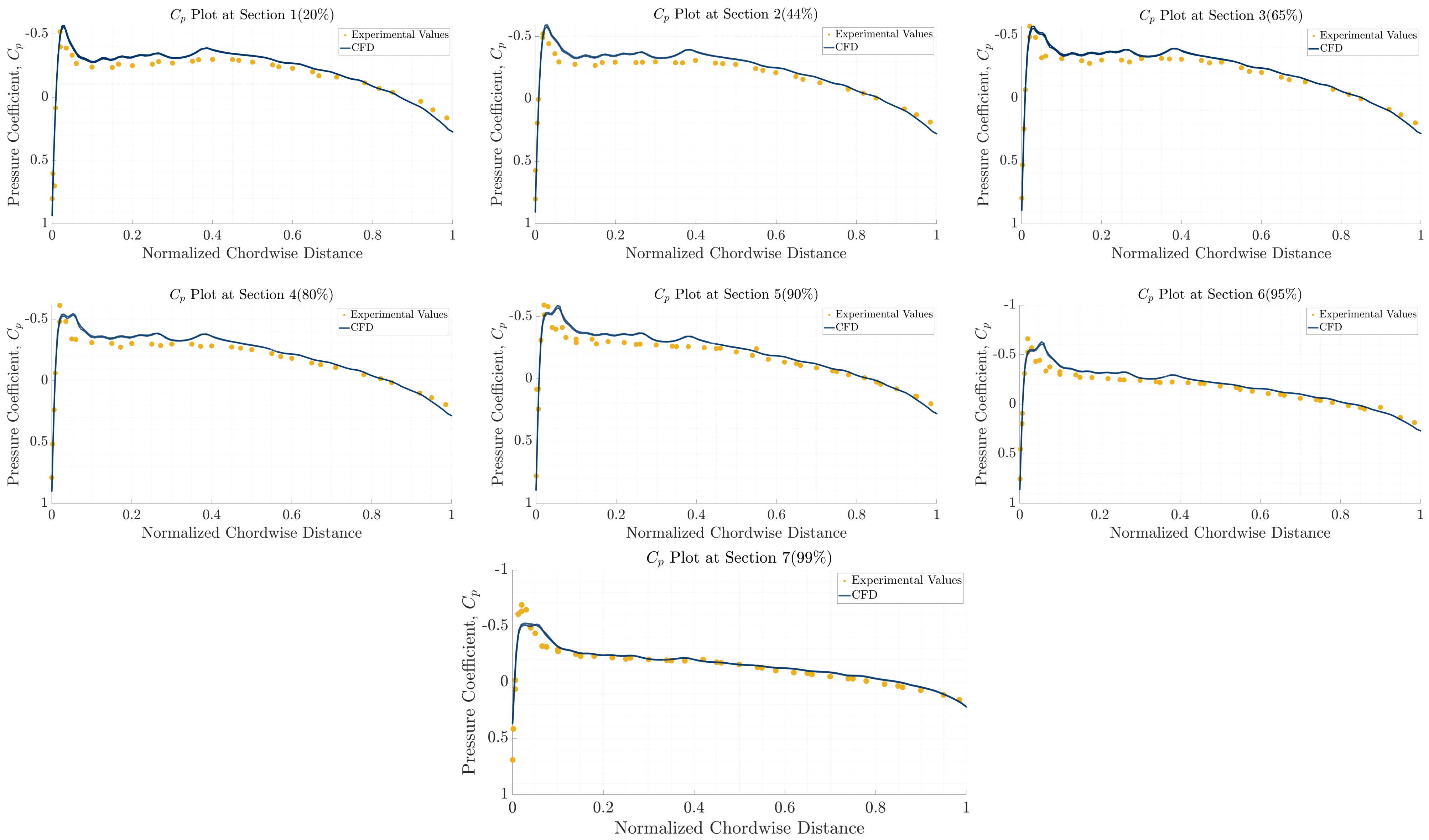
The validity of the high-fidelity CFD models setup developed within this study was investigated on the ONERA M6 transonic wing. Numerical fluid flow simulations were performed with the relevant boundary conditions and dimensions of the domain illustrated in Figure A17. Regarding the solution process, a pressure-based coupled solver was applied, with second-order spatial discretization schemes selected for all variables. Gradient information was constructed via the least-squares method, while turbulence modeling was also introduced by the Spalart–Allmaras one-equation model with a Y + 40 . The results obtained for high-fidelity aerodynamics tools were compared with the experimental values reported in [38], consisting of pressure-coefficient values measured at seven spanwise cross-sections of the wing as demonstrated in Figure A18. The results are presented in Figure A19. A mesh convergence study was also conducted, with the major aerodynamic coefficients, denoted as C L , C D and C M , respectively; these are compared in Table A1. As a general trend, pressure coefficients for both numerical models are in good accordance with the experimental values.
Figure A17. ONERA M6 CFD domain dimensions and boundary conditions.
Drones 10 00352 g0a17
Figure A18. ONERA M6 pressure coefficient measurements spanwise sections.
Drones 10 00352 g0a18
Figure A19. Pressure coefficient comparison at each spanwise station.
Drones 10 00352 g0a19
Table A1. ONERA M6 wing CFD convergence analysis.
nr of Cells C L C D C M
2 × 10 6 0.27470.0209−0.1997
4.8 × 10 6 0.27520.0189−0.1990
7 × 10 6 0.27790.0181−0.2015

References

  1. Lyu, Z.; Kenway, G.K.W.; Martins, J.R.R.A. Aerodynamic Shape Optimization Investigations of the Common Research Model Wing Benchmark. AIAA J. 2015, 53, 968–985. [Google Scholar] [CrossRef]
  2. Chen, S.; Lyu, Z.; Kenway, G.K.W.; Martins, J.R.R.A. Aerodynamic Shape Optimization of Common Research Model Wing–Body–Tail Configuration. J. Aircr. 2016, 53, 276–293. [Google Scholar] [CrossRef]
  3. Ghafoorian, F.; Wan, H.; Chegini, S. A Systematic Analysis of a Small-Scale HAWT Configuration and Aerodynamic Performance Optimization Through Kriging, Factorial, and RSM Methods. J. Appl. Comput. Mech. 2024, 11, 887–903. [Google Scholar] [CrossRef]
  4. Zheng, B.; Moni, A.; Yao, W.; Xu, M. Manifold Learning for Aerodynamic Shape Design Optimization. Aerospace 2025, 12, 258. [Google Scholar] [CrossRef]
  5. Kilimtzidis, S.; Dimitriadis, G.; Kostopoulos, V. A Novel Surrogate-Assisted Structural Optimization Framework for Full-Aircraft Configurations. In Proceedings of the AIAA SCITECH 2026 Forum, Orlando, FL, USA, 12–16 January 2026. [Google Scholar] [CrossRef]
  6. Kilimtzidis, S.; Kotzakolios, A.; Kostopoulos, V. Efficient structural optimisation of composite materials aircraft wings. Compos. Struct. 2023, 303, 116268. [Google Scholar] [CrossRef]
  7. Miki, M.; Sugiyama, Y. Optimum design of laminated composite plates using lamination parameters. AIAA J. 1993, 31, 921–927. [Google Scholar] [CrossRef]
  8. Fukunaga, H.; Sekine, H.; Sato, M. Bending-twisting coupling effects on the fundamental frequency of laminated composite plates. Compos. Struct. 1994, 28, 355–362. [Google Scholar]
  9. Liu, B.; Haftka, R.T.; Akgun, M.A. Two-level composite wing structural optimization using lamination parameters. Struct. Multidiscip. Optim. 2004, 26, 329–341. [Google Scholar] [CrossRef]
  10. Calderon, D.E.; Mader, C.A.; Martins, J.R.R.A. Aeroelastic tailoring of a high-aspect-ratio wing using geometrically nonlinear analysis. AIAA J. 2018, 56, 4021–4036. [Google Scholar]
  11. Calderon, D.E.; Mader, C.A.; Martins, J.R.R.A. Impact of geometric nonlinearities on aircraft wing structural optimization. Struct. Multidiscip. Optim. 2019, 60, 159–176. [Google Scholar]
  12. Triplett, W.E. A Multidisciplinary Approach to Aeroelastic Optimization. Ph.D. Thesis, U.S. Air Force Institute of Technology, Wright-Patterson AFB, OH, USA, 1980. [Google Scholar]
  13. Love, M.H.; Bohlman, J.D. Aeroelastic optimization of composite wings. J. Aircr. 1989, 26, 918–924. [Google Scholar]
  14. Haftka, R.T. Optimization of flexible wing structures. J. Aircr. 1973, 10, 725–731. [Google Scholar]
  15. Haftka, R.T. Integrated aerodynamic-structural design. AIAA J. 1977, 15, 350–356. [Google Scholar]
  16. Grossman, B.; Strauch, G.J.; Eppard, W.M. Integrated aerodynamic-structural design of a sailplane wing. J. Aircr. 1988, 25, 855–861. [Google Scholar] [CrossRef]
  17. Grossman, B.; Haftka, R.T.; Kao, P.J. Integrated aerodynamic-structural optimization using sensitivity derivatives. J. Aircr. 1990, 27, 985–992. [Google Scholar]
  18. Reuther, J.J.; Alonso, J.J.; Jameson, A. Aerodynamic-structural optimization of wing shapes for Euler flow. AIAA J. 1999, 37, 312–320. [Google Scholar]
  19. Maute, K.; Allen, M.; Ramm, E. Coupled aeroelastic optimization of flexible wings. AIAA J. 2001, 39, 2055–2064. [Google Scholar]
  20. Martins, J.R.R.A.; Alonso, J.J.; Reuther, J.J. High-fidelity aero-structural design optimization of a supersonic business jet. J. Aircr. 2004, 41, 523–530. [Google Scholar] [CrossRef]
  21. Barcelos, M.; Maute, K. A Schur-Newton-Krylov solver for steady-state aeroelastic analysis. AIAA J. 2006, 44, 629–640. [Google Scholar]
  22. Barcelos, M.; Maute, K. Integrated aeroelastic optimization using RANS-based CFD. Comput. Struct. 2008, 86, 1193–1207. [Google Scholar]
  23. Kenway, G.K.W.; Martins, J.R.R.A. Multipoint high-fidelity aerostructural optimization of aircraft configurations. J. Aircr. 2014, 51, 144–160. [Google Scholar] [CrossRef]
  24. Gray, J.S. High-Fidelity Aerostructural Optimization of Aircraft Wings. Ph.D. Thesis, University of Michigan, Ann Arbor, MI, USA, 2021. [Google Scholar]
  25. Nikolaou, E.; Kilimtzidis, S.; Kostopoulos, V. Winglet Design for Aerodynamic and Performance Optimization of UAVs via Surrogate Modeling. Aerospace 2025, 12, 36. [Google Scholar] [CrossRef]
  26. Benaouali, A.; Kachel, S. Multidisciplinary design optimization of aircraft wing using commercial software integration. Aerosp. Sci. Technol. 2019, 92, 766–776. [Google Scholar] [CrossRef]
  27. Nikolaou, E.; Kilimtzidis, S.; Kostopoulos, V. Multi-Fidelity Surrogate-Assisted Aerodynamic Optimization of Aircraft Wings. Aerospace 2025, 12, 359. [Google Scholar] [CrossRef]
  28. Ansys, Inc. Ansys Fluent User’s Guide; Ansys, Inc.: Canonsburg, PA, USA, 2025. [Google Scholar]
  29. Spalart, P.; Allmaras, S. A one-equation turbulence model for aerodynamic flows. In Proceedings of the 30th Aerospace Sciences Meeting and Exhibit; American Institute of Aeronautics and Astronautics: Reston, VA, USA, 1992. [Google Scholar] [CrossRef]
  30. MSC Software. MSC/NASTRAN 2021.4 Linear Static Analysis User’s Guide; MSC Software: Newport Beach, CA, USA, 2021. [Google Scholar]
  31. Kassapoglou, C. Design and Analysis of Composite Structures; John Wiley & Sons Ltd.: Hoboken, NJ, USA, 2013. [Google Scholar] [CrossRef]
  32. Marlett, K. HEXCEL 8552 IM7 Unidirectional Prepreg 190 gsm 35% RC Qualification Statistical Analysis Report; Rept. NCP-RP-2009-028 Rev B; Technical report; National Institute for Aviation Research: Wichita, KS, USA, 2011. [Google Scholar]
  33. Alexandrov, N.M.; Dennis, J.E.; Lewis, R.M.; Torczon, V. A trust-region framework for managing the use of approximation models in optimization. Struct. Optim. 1998, 15, 16–23. [Google Scholar] [CrossRef]
  34. McKay, M.D.; Beckman, R.J.; Conover, W.J. Comparison of Three Methods for Selecting Values of Input Variables in the Analysis of Output from a Computer Code. Technometrics 1979, 21, 239–245. [Google Scholar] [CrossRef]
  35. Jones, D.R. A Taxonomy of Global Optimization Methods Based on Response Surfaces. J. Glob. Optim. 2001, 21, 345–383. [Google Scholar] [CrossRef]
  36. Forrester, A.I.J.; Sóbester, A.; Keane, A.J. Engineering Design via Surrogate Modelling; Wiley: Hoboken, NJ, USA, 2008. [Google Scholar] [CrossRef]
  37. Forrester, A.I.; Sóbester, A.; Keane, A.J. Multi-fidelity optimization via surrogate modelling. Proc. R. Soc. A Math. Phys. Eng. Sci. 2007, 463, 3251–3269. [Google Scholar] [CrossRef]
  38. Schmitt, V.; Charpin, F. Pressure Distributions on the ONERA-M6-Wing at Transonic Mach Numbers; Technical report; Advisory Group for Aerospace Research and Development, North Atlantic Treaty Organization: Neuilly-sur-Seine, France, 1979. [Google Scholar]
Figure 1. Baseline UAV configuration.
Drones 10 00352 g001
Figure 2. CFD domain characteristics (Purple surfaces: Inlets, Orange surface: Outlet, Grey surface: Symmetry).
Drones 10 00352 g002
Figure 3. CFD mesh around the wing.
Drones 10 00352 g003
Figure 4. C L and C D vs. number of domain cells—mesh independence study.
Drones 10 00352 g004
Figure 5. Y + distribution—mesh independence study.
Drones 10 00352 g005
Figure 6. MSC NASTRAN FEM model mesh of the wing.
Drones 10 00352 g006
Figure 7. Parametric CFD-FEM modeling framework.
Drones 10 00352 g007
Figure 8. General SBO framework.
Drones 10 00352 g008
Figure 9. Convergence of cumulative best feasible range over evaluations for five SBO iterations.
Drones 10 00352 g009
Figure 10. Wing top view of the optimized configurations of each SBO iteration.
Drones 10 00352 g010
Figure 11. CFD Aerodynamic results for each best wing configuration of the 5 SBO iterations— C L (a), C D (b), C m (c), and L / D (d) vs. AoA.
Drones 10 00352 g011
Figure 12. Fifth SBO iter.—correlation between objective and constraints.
Drones 10 00352 g012
Figure 13. Fifth SBO iter.—correlation of aerodynamic and structural design parameters with Range-Objective.
Drones 10 00352 g013
Figure 14. Fifth SBO iter.—correlation of aerodynamic and structural design parameters with L / D (a), and W e i g h t (b).
Drones 10 00352 g014
Figure 15. Fifth SBO iter.—correlation of aerodynamic and structural design parameters with g 1 (a), g 2 (b), g 3 (c), and g 4 (d).
Drones 10 00352 g015
Figure 16. Y + contours on upper (a), and lower (b) wing surfaces of the selected optimized configuration.
Drones 10 00352 g016
Figure 17. Pressure coefficient (a), and temperature (b) contours of surfaces of the selected optimized configuration.
Drones 10 00352 g017
Figure 18. Velocity pathlines around the wing of the selected optimized configuration. (Side view (a), Isometric view (b), Front view (c), and Top view (d) of the wing).
Drones 10 00352 g018
Figure 19. Deformed shape contour (m) of the selected optimized configuration.
Drones 10 00352 g019
Figure 20. Maximum FI contour of the selected optimized configuration.
Drones 10 00352 g020
Figure 21. Maximum beam stresses contour (MPa) of the selected optimized configuration.
Drones 10 00352 g021
Table 1. UAV requirements and mission flight characteristics.
CharacteristicSymbol
UAV typeFixed-wing
Propulsion systemBattery-powered electric
Wingspan≤3 m
UAV length≤1.5 m
Maximum take-off weight≤15 kg
Take-offCatapult take-off
Cruise speed≥22 m/s
Loiter Speed≥20 m/s
Climb Speed 1.2 × V s t a l l
Operational altitude1500 m A S L
Table 2. Composite materials properties [32].
Material SystemHexcel IM7/8552
E 1 , GPa158.51
E 2 , GPa8.96
G 12 , GPa4.68
G 23 , GPa3.98
ν 12 0.31
ν 23 0.435
X T , MPa2500
X C , MPa1531
Y T , MPa640.5
Y C , MPa285.7
S, MPa53.5
Ply thickness, m 1.8288 × 10 4
Table 3. Optimization variables bounds.
VariableLower BoundUpper Bound
Aspect Ratio ( A R )6.515
Taper Ratio ( λ )0.21
Quarter-chord sweep angle ( Λ ), d e g 0 15
Twist ( ϵ ), d e g 4 4
Front Spar Location ( F S L ), % C 0.150.3
Rear Spar Location ( R S L ), % C 0.60.75
Rib Spacing ( R S ), % b / 2 0.10.3
Stringer Spacing ( S S ), % C 0.10.3
Upper Skin Thickness ( U S T ), mm0.20.6
Lower Skin Thickness ( L S T ), mm0.20.6
Front Spar Thickness ( F S T ), mm0.20.6
Rear Spar Thickness ( R S T ), mm0.20.6
Ribs Thickness ( R T ), mm0.20.6
Table 4. Optimization problem summary.
Objective FunctionMaximize Range
Constraint TypeConstraint Equation
C L c r u i s e ( g 1 ) 0.8 g 1 0
F I m a x , Shell Elements ( g 2 ) g 2 1 0
FoS, Beam Elements ( g 3 ) 1.5 g 3 0
Linear Buckling Eigenvalue ( g 4 ) 1.5 g 4 0
Table 5. Surrogate model accuracy across five independent SBO runs.
RunRMSE R 2
1 5.658 1.8030
2 5.972 0.9019
3 7.312 0.9225
4 4.772 0.9343
5 4.399 0.9678
Mean ± SD 5.62 ± 1.11 0.3847 ± 1.2503
Table 6. Leave-One-Out (LOO) cross-validation accuracy of the surrogate models.
RunMax|Error|RMSELOO R LOO 2
1 2.747 × 10 1 7.934 × 10 0 0.8213
2 3.264 × 10 1 8.806 × 10 0 0.8161
3 2.746 × 10 1 7.833 × 10 0 0.8258
4 3.709 × 10 1 8.582 × 10 0 0.8112
5 2.327 × 10 1 8.411 × 10 0 0.8167
Mean ± SD 2.959 × 10 1 ± 5.350 × 10 0 8.313 × 10 0 ± 4.183 × 10 1 0.8182 ± 0.0056
Table 7. Best configurations of all iterations.
Objective and Constraints Results
SBO Iter.L/DWRg1g2g3g4
126.5040.829196.817−0.021−0.886 1.2 × 10 5 −0.013
225.5180.828189.519−0.043−0.882 2.2 × 10 5 −0.099
325.7520.829191.232−0.004−0.887 1.7 × 10 5 −0.192
425.6420.832190.336−0.024−0.897 1.0 × 10 5 −0.240
527.2920.823202.838−0.023−0.877 2.2 × 10 5 −0.075
Aerodynamic Design Parameters
SBO Iter.AR λ Λ ε
113.930.223.55−0.40
212.630.342.292.11
312.830.285.760.31
413.090.230.901.48
514.860.448.850.06
Structural Design Parameters
SBO Iter.FSLRSLRSSSUSTLSTRSTRT
10.2790.6620.2580.1860.000520.000400.000500.00043
20.2910.6450.2420.2640.000520.000240.000500.00052
30.2670.6090.2450.1550.000490.000550.000570.00031
40.2620.6660.1560.1210.000530.000410.000360.00023
50.2550.6780.1200.2870.000440.000500.000570.00031
Table 8. SBO 5th iteration—best possible configurations results of samples.
A/A L / D WR g 1 g 2 g 3 g 4
Samples
922.6220.846167.593−0.008−0.928 2.9 × 10 5 −0.437
2319.5520.773146.341−0.024−0.889 1.8 × 10 5 −0.042
2618.7960.802140.103−0.022−0.826 3.8 × 10 5 −0.077
4226.4630.811197.000−0.043−0.913 5.1 × 10 5 −0.811
4925.9010.813192.770−0.056−0.880 6.6 × 10 5 −0.077
5024.2730.782181.443−0.074−0.909 5.1 × 10 6 −0.488
5820.3400.796151.737−0.013−0.871 2.6 × 10 5 −0.025
6018.4990.805137.829−0.041−0.918 5.3 × 10 5 −0.699
6625.7610.808191.868−0.025−0.851 1.8 × 10 6 −0.289
7017.8260.794133.026−0.042−0.938 3.7 × 10 5 −1.268
7824.9810.814185.914−0.038−0.915 8.7 × 10 5 −0.789
8327.2920.823202.838−0.023−0.877 2.2 × 10 5 −0.075
8724.4560.846181.177−0.002−0.897 2.2 × 10 5 −0.220
Table 9. SBO 5th iteration—best possible configurations results of infills.
A/A L / D WR g 1 g 2 g 3 g 4
Infills
217.7130.814131.807−0.035−0.900 1.9 × 10 5 −0.164
617.7990.800132.723−0.037−0.896 1.7 × 10 5 −0.098
817.7670.812132.241−0.034−0.861 4.0 × 10 5 −0.009
924.2890.814180.752−0.040−0.892 2.2 × 10 5 −0.168
1017.5560.802130.875−0.046−0.892 1.4 × 10 5 −0.085
1317.3950.811129.499−0.041−0.862 2.3 × 10 5 −0.039
1417.9480.799133.838−0.032−0.896 1.5 × 10 5 −0.097
1724.8170.813184.707−0.047−0.885 2.0 × 10 5 −0.094
1822.6140.829167.938−0.008−0.925 9.5 × 10 5 −0.523
1922.5880.824167.851−0.018−0.917 8.7 × 10 5 −0.417
2322.5960.825167.897−0.015−0.920 8.3 × 10 6 −0.420
2522.6010.826167.913−0.012−0.922 2.3 × 10 6 −0.458
3423.0950.797172.268−0.047−0.893 2.6 × 10 5 −0.036
3516.7990.799125.275−0.011−0.906 4.3 × 10 5 −0.228
3617.6520.792131.760−0.040−0.931 5.4 × 10 5 −1.055
3722.6710.823168.493−0.003−0.918 9.3 × 10 5 −0.360
3822.6680.823168.469−0.003−0.918 8.7 × 10 5 −0.340
3923.1080.809172.076−0.031−0.892 1.3 × 10 6 −0.032
4022.7660.823169.202−0.009−0.914 2.4 × 10 5 −0.349
4123.1130.809172.115−0.030−0.892 4.3 × 10 5 −0.024
4222.8160.817169.719−0.009−0.914 5.0 × 10 5 −0.197
4322.7640.823169.175−0.009−0.914 1.7 × 10 6 −0.349
4422.7850.819169.443−0.009−0.915 6.1 × 10 5 −0.354
4523.0820.810171.870−0.030−0.894 6.9 × 10 5 −0.050
4623.0560.810171.674−0.029−0.894 4.1 × 10 5 −0.048
4722.8000.818169.571−0.010−0.915 5.9 × 10 5 −0.300
4823.0780.810171.840−0.029−0.894 7.9 × 10 5 −0.054
5622.7940.818169.537−0.009−0.914 6.3 × 10 5 −0.345
5823.2170.809172.894−0.032−0.930 3.8 × 10 5 −1.077
6017.7440.799132.318−0.044−0.893 3.2 × 10 5 −0.008
Disclaimer/Publisher’s Note: The statements, opinions and data contained in all publications are solely those of the individual author(s) and contributor(s) and not of MDPI and/or the editor(s). MDPI and/or the editor(s) disclaim responsibility for any injury to people or property resulting from any ideas, methods, instructions or products referred to in the content.