A Method of Deep Mineralization Potential Exploration Based on UAVs and Its Application in an Abandoned Mine in the Democratic Republic of the Congo

Highlights

What are the main findings?

• Semi-airborne transient electromagnetic exploration based on a UAV can reach a detection depth of over 600 m and simultaneously obtain resistivity and chargeability information.
• By analyzing the detection results in combination with geological data, a low-resistance and high-polarization zone was discovered, which provides clues for the exploration of deep deposits.

What are the implications of the main findings?

• This technology provides an innovative solution for deep and high-resolution exploration of mineral resources under complex terrain conditions.
• This method highlights the application potential of UAV-based electromagnetic technology in greenfield and brownfield exploration.

Abstract

In recent years, unmanned aerial vehicles (UAVs) have increasingly become carrying platforms for Earth observation systems equipped with optical, microwave, and other types of sensors, primarily enabling high-resolution observations of above-ground targets. With the development of geophysical methods, bulky instruments originally designed for deep subsurface detection have been progressively miniaturized and made more lightweight, allowing their integration with civilian UAVs and opening new technological avenues for subsurface investigation. We have developed a semi-airborne transient electromagnetic system based on a UAV that is capable of simultaneously obtaining underground resistivity and polarization rate parameters. A survey was conducted over the M’sesa mining area in the Democratic Republic of the Congo. This is a mine pit that has been abandoned for over 50 years and has been flooded to form a lake, making it difficult to detect its deep mineralization potential using traditional ground-based methods. The results clearly delineate the spatial distribution of the Shangoluwe–M’sesa compressional fault and reveal a deep low-resistivity and high-chargeability zone, which provides clues for the exploration of deep deposits. This study will be of significant importance for accelerating the promotion and application of UAV-based semi-airborne electromagnetic exploration technologies.

1. Introduction

Mineral resource exploration in regions with complex terrain has long been a highly challenging task [1]. Deploying geophysical systems on airborne platforms enables extensive coverage over large survey areas [2,3,4,5,6]. During the development of these technologies, although unmanned aerial vehicle (UAV) technology had already been proposed [7], limitations related to the weight, volume, and power consumption of detection equipment meant that manned aircraft were predominantly used as carrying platforms in the initial phases. In recent years, with substantial advances in the miniaturization and lightweight design of detection equipment, together with the rapid development of heavy-duty civilian UAVs, an increasing number of studies have favored UAVs as carrying platforms for mineral exploration systems [8,9].

Among the methods available for metallic mineral exploration, the controlled-source electromagnetic (CSEM) method is one of the most widely applied techniques [10]. This method uses a long-grounded wire or closed loop as the transmitting antenna to excite the subsurface and extract the distribution of earth resistivity parameters from the measured earth response signals. In traditional CSEM systems, all detection equipment is deployed on the ground. Complex topographic conditions will lead to a significant reduction in survey efficiency and even make surveys difficult to complete. The airborne electromagnetic (AEM) method is the airborne version of the conventional ground-based method, in which all detection equipment is mounted on fixed-wing aircraft or helicopters [2,11,12,13], thereby significantly enhancing the method’s usability in complex terrain scenarios. However, because the excitation energy delivered to the subsurface by such systems is entirely constrained by the power supply capacity of the carrying platform, their investigation depth is limited to some extent. In addition, the use of manned aircraft as carrying platforms is economically unfeasible for the vast majority of small- and medium-sized mines. To address this issue, semi-airborne electromagnetic (SAEM) methods, as a compromise between ground-based methods and AEM, have developed rapidly in recent years. The SAEM system deploys high-power transmitting equipment (including the transmitter, the transmitting antenna and the high-power generator specifically for powering the transmitter) on the ground. Since only the limited-weight receiving device (including the receiver and sensors) needs to be carried, ordinary civilian UAVs can be used as the carrying platform. This system design will achieve a balance of detection depth and convenience [14,15,16,17].

Over the past decade, in parallel with the rapid rise of UAV technology, SAEM has gradually gained broader recognition in the market [18]. Under conventional conditions, the SAEM system can yield one physical property parameter of the earth, namely, the earth’s resistivity. However, in the detection of metallic mines, the induced polarization effect (IPE) [19] is widely present, which will lead to a deviation between the resistivity results obtained from the survey and the actual situation [20]. The IPE is an electrochemical phenomenon, the essence of which is that rocks, influenced by multiple factors, such as the degree of mineralization, porosity, multiphase mineral assemblages, anisotropy, and fluid content, exhibit low-frequency dispersion behavior in their electrical resistivity [21,22]. From another perspective, however, the occurrence of the IPE can also be regarded as providing distinctive indicators for specific targets, such as disseminated mineralization or conductive clays [23,24,25]. Taking into full account that the physical processes of the IPE and electromagnetic response are different, extracting resistivity and chargeability parameters from the data through inversion methods will be conducive to obtaining more reliable geological interpretations [26].

We have conducted research on the aforementioned issues and developed the DROEM, a semi-airborne transient electromagnetic (SATEM) system. The DROEM system adopts a denoising method based on deep learning, which is less affected by human factors. Moreover, the DROEM system can simultaneously extract resistivity and polarization rate parameters. Compared with systems that can only provide resistivity parameters, it is more conducive to subsequent geological interpretation work. A survey was carried out over the abandoned M’sesa mine pit located in the Kambove area of the Democratic Republic of the Congo, with the aim of assessing its deep mineralization potential. M’sesa is a mine that was closed in the 1970s. In recent years, sulfide orebodies have been discovered beneath the shallow oxidized orebodies in several currently operating mines around M’sesa, such as Kambove and Kamoya [27,28]. This has raised a question: Is it possible that there are sulfide ores in the deep part of M’sesa as well? However, as the M’sesa mine has been abandoned for many years, there is a lack of deep exploration data. Moreover, a large amount of water has accumulated in the mine pit, forming a lake, which makes it difficult to carry out ground exploration work. We used the DROEM system to conduct detection work in an area of approximately 4 square kilometers, and the flight mission was completed within 3 h. We processed the data and obtained the resistivity and chargeability results of the survey area. The survey results clearly reveal the shape of the Shangoluwe–M’sesa compressional fault in the depth direction and can be well matched with the known geological data. In addition, a low-resistivity–high-chargeability zone was identified in the deep part on the east side of the fault. Combined with geological analysis, this discovery may constitute a certain clue for the exploration of deep deposits, which will provide a reference for the subsequent drilling and development work. This study will be of significant importance for accelerating the promotion and application of UAV-based SAEM exploration technologies.

2. Materials and Methods

2.1. Geological Setting

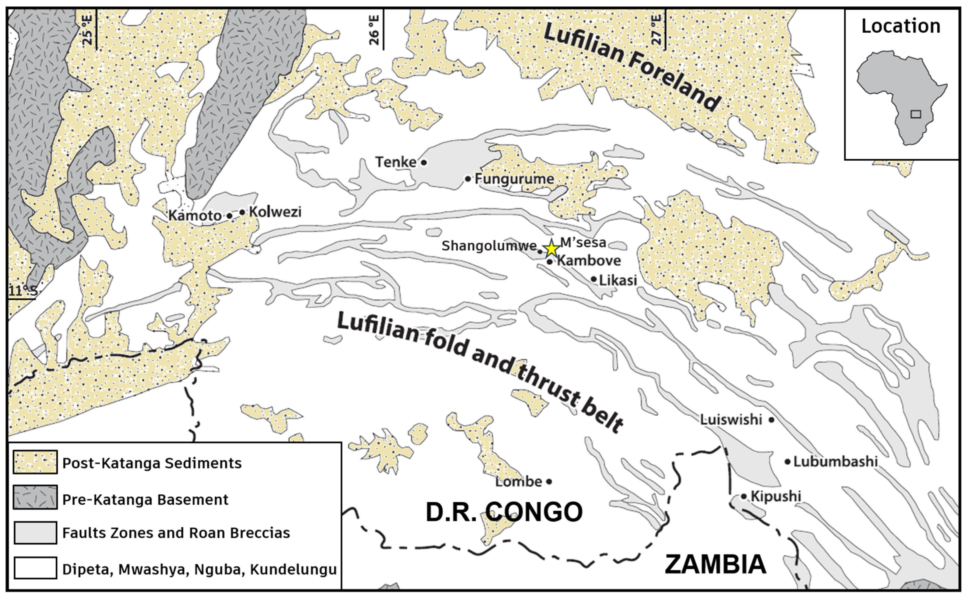
As shown in Figure 1, the M’sesa mining area is located in Kambove Territory, Haut-Katanga Province, Democratic Republic of the Congo, and lies in the north-central part of the Central African Copperbelt (CACB). The CACB is generally characterized by a northeast-convex arcuate geometry, extending for approximately 700 km in length and 50–150 km in width, and represents the world’s largest and most prolific sediment-hosted stratiform Cu-Co belt [29,30,31]. The CACB comprises five tectonic domains [32], namely, the Outer Lufilian (external fold-and-thrust belt), Middle Lufilian (Domes region), Inner Lufilian (synclinorial belt), Katanga High, and the Katangan aulacogen. The M’sesa deposit is situated within the Katanga Basin of the Outer Lufilian domain, where the exposed Neoproterozoic Katanga Supergroup consists of a 5–10 km thick succession of metamorphosed sedimentary rocks [33]. Sediment-hosted Cu-Co mineralization is mainly hosted in the Roan Group at the base of the Neoproterozoic Katanga Supergroup. Specifically, the Roan Group includes four subgroups: Musonoï (R1), Mines (R2), Fungurume (R3), and Mwashya (R4), among which the Mines Subgroup is the most economically significant [34]. The Mines (R2) Subgroup is further subdivided into three formations: Kamoto (R2.1), Kinsevere (R2.2), and Kambove (R2.3). In the study area, the principal ore-hosting horizons occur in the middle (RSF, R2.1.2) and upper (RSC, R2.1.3) parts of the Kamoto Formation (R2.1), as well as in the lower (SDB, R2.2.1) and middle (SDS, R2.2.2) parts of the Kinsevere Formation (R2.2). It is generally considered that the Lufilian orogeny occurred in this region between approximately 592 ± 22 Ma and 512 ± 17 Ma [35]. During the orogenic event, fracturing and fluid migration promoted the enrichment and remobilization of metals such as copper, gold, platinum, and cobalt [36], constituting the main driving mechanism for mineral accumulation. In addition, the sedimentary sequences of the Katanga Basin were deformed during the Lufilian orogeny, forming predominantly north-dipping folds, thrust faults, and thrust nappes [37], which represent the principal ore-controlling geological factors in this region.

The M’sesa Cu–Co deposit is a stratabound deposit modified by mixed hydrothermal processes. During the early mineralization stage, large amounts of metal sulfides were generated and accumulated. Subsequent fault activity provided space for hydrothermal modification, and later tectonic activity promoted oxidation and re-enrichment of surface and near-surface sulfide minerals through weathering and leaching processes, thereby forming oxide orebodies at the surface [31]. Within the M’sesa mining area specifically, a major regional strike–slip fault with an NNW-SSE trend is exposed. This fault is approximately 6.2 km long, exhibits a wavy geometry, and is distributed in the central-western part of the mining area, extending continuously from south to north. It dips westward and is nearly vertical in attitude, while at depth it cuts strata at a sharp angle, giving the overall structure a plow-shaped geometry. During the development of the thrust–nappe structure, relative displacement and compressional deformation occurred along the margins of individual blocks, forming unconformable slip surfaces. The associated fault damage zones commonly consist of breccias with a certain degree of rounding. These breccias were previously described as tectonic breccias or gravity breccias [38]. In recent years, however, some researchers have reinterpreted them as sedimentary breccias [39,40].

Figure 1. Geological map of the CACB (edited based on [41,42]).

Figure 1. Geological map of the CACB (edited based on [41,42]).

2.2. Data Acquisition

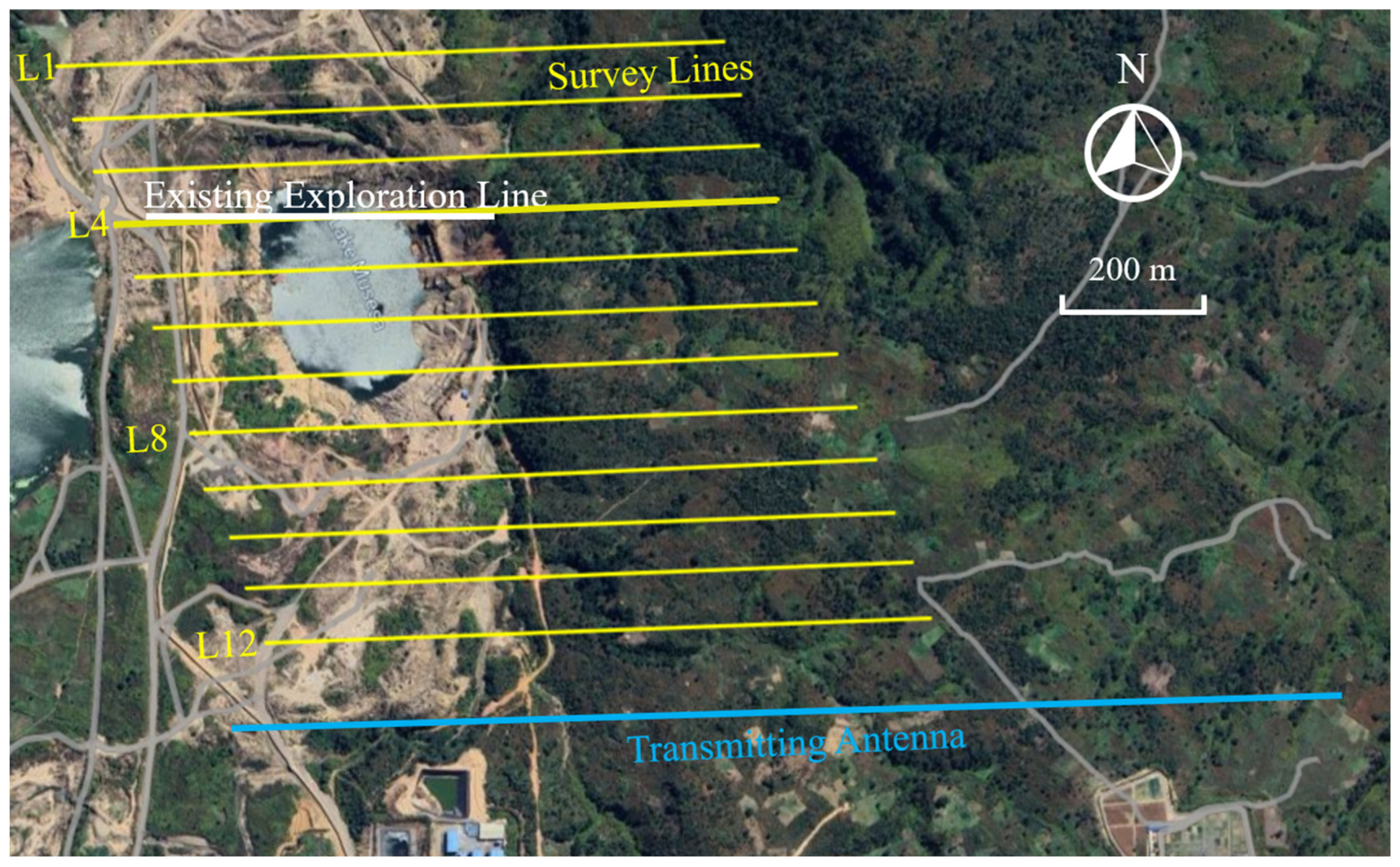
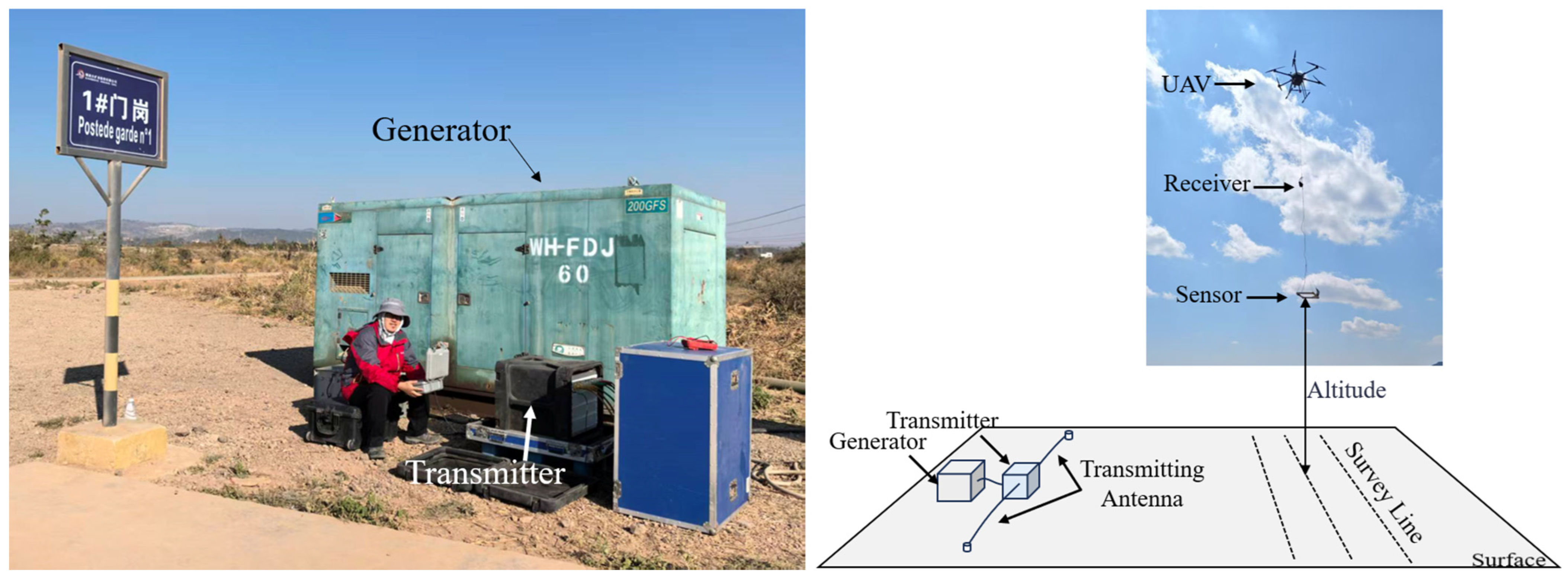
As shown in Figure 2, the core of the survey area is the M’sesa mine pit, which is located to the north of the current Kambove mine plant area. Historically, the pit produced nearly 500,000 tonnes of ore, approximately half of which was copper ore, with an average grade of about 5%. Since the 1970s, the surrounding surface drainage system has continuously drained into the pit, resulting in the formation of a lake. In 2024, the owner of the mining rights carried out dewatering operations within the pit, and the water level dropped by 50 m. Additionally, there is about 40 m of silt beneath the lake bottom. Under such conditions, further investigation of deep mineralization potential using conventional ground-based methods remains highly challenging. Therefore, the SAEM method was adopted to provide survey coverage over the target area. The Shangoluwe–M’sesa shear zone generally trends in a north–south direction, which was the main directional basis for us when setting up the detection equipment. In Figure 3, the field equipment and layout method we used are presented. The transmitting device mainly consists of a transmitter, a generator and a transmitting antenna. The transmitting antenna uses a common multi-core copper wire with a cross-sectional area of 6 mm². The transmitting antenna is placed on the ground surface, with one end connected to the earth through aluminum foil and the other end connected to the transmitter, thus forming a loop with the transmitter, the transmitting antenna and the ground. The layout direction of the transmitting antenna is generally perpendicular to the structural trend, that is, in the east–west direction, and the distance between the two grounding points is 2 km. In this survey, the output current waveform is a bipolar square wave, with a peak current amplitude of 25 ± 0.2 A and a pulse repetition frequency of 25 Hz. According to Faraday’s law of electromagnetic induction, the actual excitation effect of the transient electromagnetic method on the earth is generated during the turn-on or -off process of the square wave. This process usually lasts for several tens of microseconds, and its bandwidth is much greater than the repetition frequency of the square-wave pulse. The reason for choosing transmitting base frequencies such as 25 Hz is mainly to meet the bipolar synchronous sampling method proposed by Macnae et al. to suppress power-line interference [43]. We set up the transmitting antenna on the south side of the survey area and covered the area with 12 survey lines that were parallel to the transmitting antenna, each 1200 m long and spaced 100 m apart. The DROEM observation system consists of a receiver and a sensor (Z-axis inductive coil) and is suspended beneath the UAV by Kevlar cables. The receiver adopts a 100 kHz, 32-bit analog-to-digital converter (ADC) and is synchronized with the transmitter via GPS. The resonant frequency of the sensor is 52 kHz, and the noise level is 0.1 nT/s. The total weight of the sensor and the receiver is 2.91 kg, and the total power consumption is 3.4 W. After the deployment of the transmitting device was completed, all the data observation work was finished in three hours, and the same amount of work would have taken more than two weeks with traditional ground-based detection.

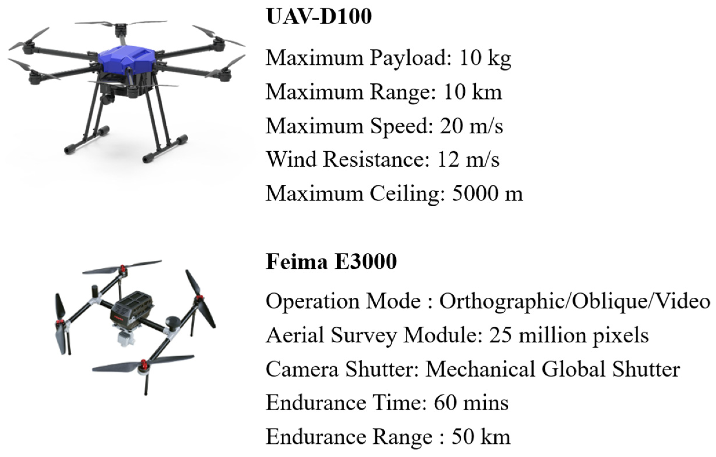
Considering multiple factors, including the relationship between the signal-to-noise ratio of integrated data, horizontal resolution and flight speed, as well as the convenience of equipment integration, a hexacopter UAV was selected as the carrying platform [26]. The sensor used here is an inductive magnetic field sensor with a resonant frequency of 52 kHz. If the sensor is directly installed on the UAV, on the one hand, the interfering electromagnetic field generated by the UAV’s motor will be detected, and on the other hand, the vibration of the UAV will induce an electromotive force in the sensor, thereby generating some kind of induced-motion noise. Currently, the commonly used solution is to suspend the sensor below the UAV at a certain distance (generally 5 to 10 m) using a cable. However, due to the suspended configuration, aerodynamic drag during flight results in a tensile force transmitted to the UAV that is significantly greater than the actual weight of the equipment. To ensure flight safety, and after fully considering the performance margin of the UAV, a customized UAV with a maximum effective payload of 10 kg (model D100; Figure 4) was selected. The effective flight time of a single sortie is approximately 30 min. When carrying the receiving equipment over the M’sesa survey area and cruising at a speed of 5 m/s, the UAV can complete at least four survey lines before the battery voltage drops to the first-level warning threshold (54.5 V). In recent years, advances in artificial intelligence have markedly enhanced UAV capabilities in battery thermal management [44,45]. UAVs will be capable of autonomously performing more complex flight tasks and have longer single flight times, thus better meeting the demands of geophysical exploration. In terms of flight mode, a constant-altitude flight strategy was adopted. For this survey, the fixed cruising altitude of the UAV was set to 1470 m (about 150 m above the ground surface). This mode was chosen instead of terrain-following flight because the latter would introduce more complex motion-induced noise. Motion-induced noise refers to the electromotive force generated by changes in magnetic flux within an inductive magnetic field sensor as it moves through a non-uniform geomagnetic field [46]. Such noise represents one of the primary noise sources in airborne electromagnetic observations, and its magnitude is often two to three orders of magnitude greater than that of the weak useful signals associated with deep exploration targets. If the motion of the sensor is relatively stable, the resulting motion-induced noise is mainly confined to low frequencies. In contrast, under terrain-following flight in areas with complex topography, the motion of the sensor suspended beneath the UAV becomes more complicated, leading to motion-induced noise with both larger amplitude and broader bandwidth. This noise then falls within the signal bandwidth, substantially increasing the difficulty of noise suppression during data processing. Accordingly, a constant-altitude flight mode was adopted to ensure a relatively simple motion pattern of the sensor in the air. However, this observation mode also introduces a new issue: the sensor–ground distance varies among different measurement points, which requires the sensor height above ground to be treated as a parameter in the inversion process. Therefore, prior to the formal survey, a small photogrammetric UAV (E3000 [47]) was used to construct a three-dimensional model of the survey area, enabling the extraction of surface elevations at each measurement point. By subtracting the surface elevation from the GPS-derived altitude of the sensor, the sensor-to-ground distance at each location was obtained.

2.3. Geophysical Information Extraction

From the acquisition of observation data to the final extraction of subsurface electrical parameters, the workflow generally involves two major steps. The first step is the processing of raw data, through which windowed decay curves are extracted for each measurement point. The second step is the inversion of these windowed decay curves to obtain the electrical parameters of the subsurface.

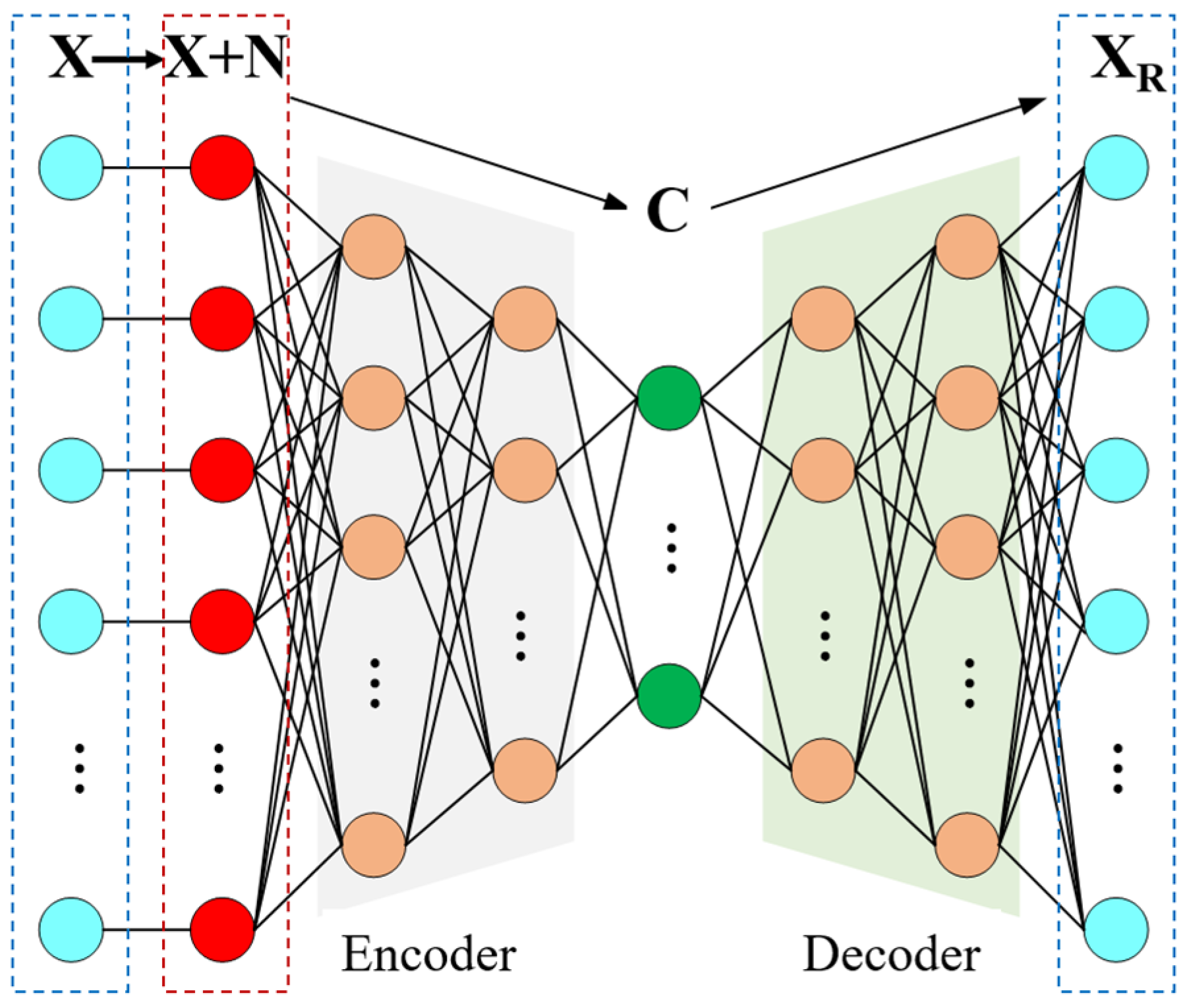
The main task of processing observational data is to remove various types of noise and output the windowed decay curves of each measurement point. Traditionally, different denoising methods are generally adopted to deal with different noises [18,48], such as motion-induced noise, sferics noise, and background noise. Because such a workflow-based processing approach involves multiple steps, each of which requires careful parameter tuning, it places high demands on the experience of the operator. To address this issue, our previous work proposed a multi-source noise processing method based on a denoising autoencoder (DAE) neural network [49]. A DAE is a type of autoencoder neural network that takes a corrupted signal as input and is trained to accurately predict the corresponding clean signal [50]. The basic architecture of the designed DAE network is shown in Figure 5. Its main design features include: 1000 samples at both the input and output ends (corresponding to a 10 ms observation window at a sampling rate of 100 kHz); four layers each in the encoder and decoder, with 100 nodes in the encoding layer; the use of rectified linear unit (ReLU) activation functions; and the mean square error (MSE) as error function.

During network training, the training dataset was constructed using a combination of synthetic signals and measured noise [51]. Specifically, to enhance generalization capability, resistivity values were selected at logarithmically equal intervals within the range of 10¹–10⁴ Ω·m, and these candidate resistivities were distributed within a depth range of 0–1500 m according to three-layer, four-layer, and five-layer subsurface models. For layers with resistivity less than 10² Ω·m, chargeability values were randomly selected within the range of 65% to 100%; for layers with resistivity in the range of 10²–10³ Ω·m, chargeability values were randomly selected within 35% to 70%; and for layers with resistivity in the range of 10³–10⁴ Ω·m, chargeability values were randomly selected within 0% to 40%. After eliminating unreasonable models (such as those with extremely thick low-resistance layers or those with two consecutive layers having a resistivity difference of less than 10%), a total of 2843 three-layer models, 9767 four-layer models, and 19,604 five-layer models were obtained. Forward modeling of these theoretical models was performed to generate synthetic signals, and measured noise was superimposed onto the synthetic signals to form the training data. Among them, 75% were used for training. The training was conducted using an NVIDIA RTX 2080Ti GPU. When the number of consecutive epochs with Loss less than 0.01 exceeds 50, the network is considered to have converged. The training time was about 68.2 h. Because the observation results of the time-domain electromagnetic method (decay curves) have the characteristic of a large dynamic range (for a single survey area, it may even exceed 120 dB), it is necessary to adjust its dynamic range before inputting it into the network. For this purpose, we designed a simple linear transformation sequence DT = T·10,000, where T is the delay time of each sampling point in the decay curve. The dynamic range of the decay curve will be compressed by multiplying the decay curve point by point with DT. Most of the time, the dynamic range of the new data obtained is roughly at the 50 dB level. For the network output sequence, dividing each point by DT can restore the dynamic range. We tested the network performance using the data from the test dataset. The average calculation time for a single measurement point was approximately 0.02 s, and the error of the processing results relative to the theoretical data was basically less than 2%. For more detailed information about DAE, such as the training settings, model validation, and quantitative performance comparison, please refer to our previous article [49]. After network convergence, the trained model can be used to process measured data, enabling the simultaneous removal of multiple types of noise.

Figure 5. A schematic diagram of the basic structure of a denoising autoencoder neural network [52], where X is the noise-free data, and N is the noisy data. Noisy data is obtained through X + N, that is, by adding noise features to the data. X_R is the reconstructed data, and C is the coding layer.

Figure 5. A schematic diagram of the basic structure of a denoising autoencoder neural network [52], where X is the noise-free data, and N is the noisy data. Noisy data is obtained through X + N, that is, by adding noise features to the data. X_R is the reconstructed data, and C is the coding layer.

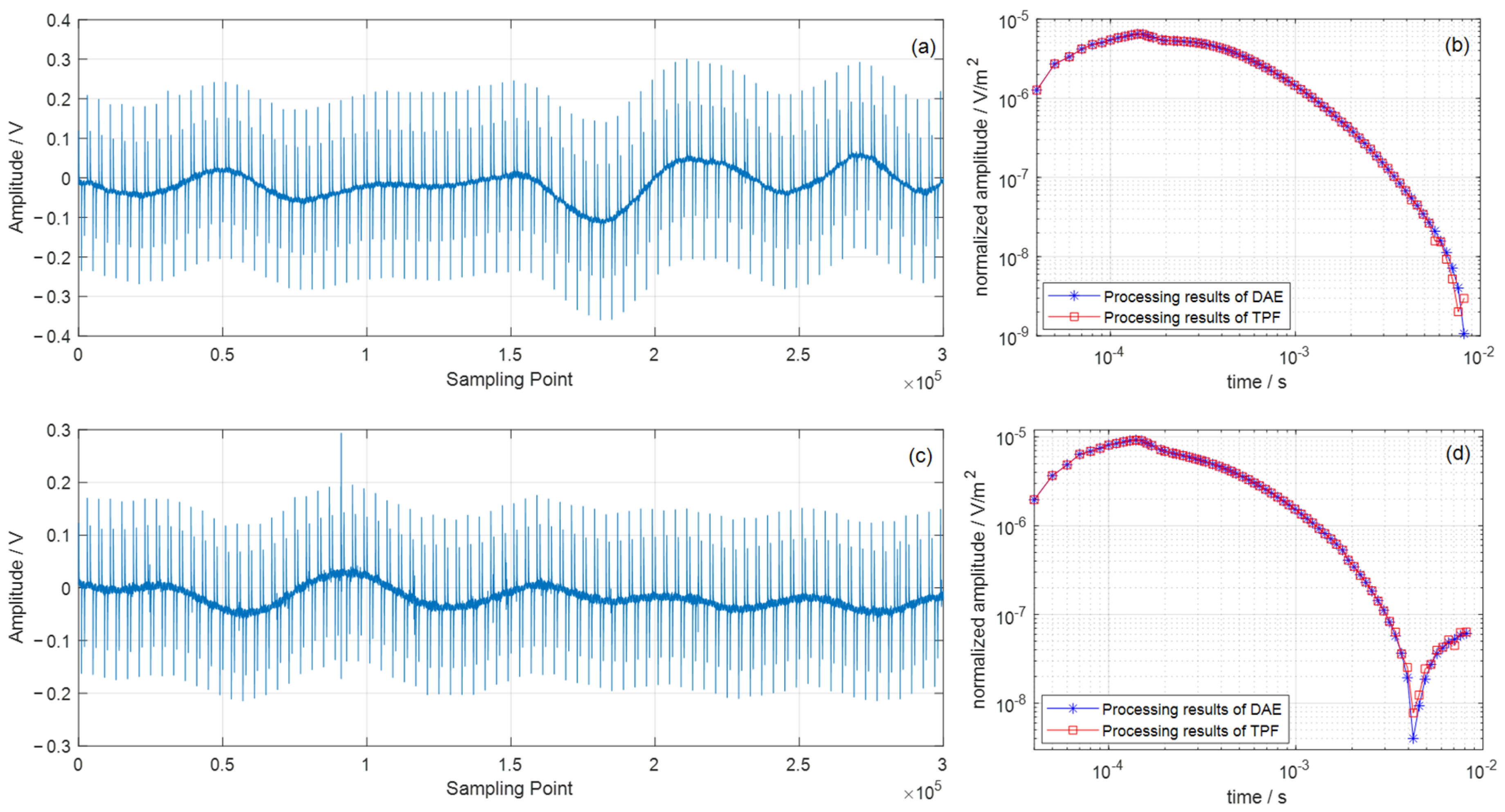
To better process the observation data acquired in the M’sesa survey area, pure-noise flight measurements were conducted during the survey (normal flight observations without activating the transmitter). The noise recorded during these flights was used to further fine-tune the pre-trained network, making it more suitable for processing signals from the current survey area. Figure 6 shows the processing results of the measured data using DAE and the traditional process-flow method (TPF) respectively. Regardless of whether induced polarization effects are present, the two methods exhibit good overall consistency. In the range from 1 × 10⁻⁴ s to 2 × 10⁻³ s, the average relative error between the two is less than 1%. In the subsequent period, the average error increases to 5%, but the continuity of the DAE processing results is higher than that of the TPF, indicating that the DAE has higher stability in processing late-stage low signal-to-noise ratio signals.

After completing data processing, inversion is performed to extract subsurface resistivity and chargeability information. Compared with the relatively mature three-dimensional electromagnetic inversion techniques, three-dimensional inversion of semi-airborne time-domain electromagnetic observations that account for induced polarization (IP) effects remains highly challenging [53]. Usually, the Cole–Cole model is used to describe the IPE [54]:

$$\sigma \left(\omega \right)={\sigma }_{\infty }\left(1-{\displaystyle \frac{\eta }{1+{\left(i\omega \tau \right)}^c}}\right)$$

(1)

where $\omega$ is the angular frequency, $\eta =({\sigma }_{\mathrm{\infty }}-{\sigma }_0)/{\sigma }_{\mathrm{\infty }}$ is the chargeability, $\tau$ is the time constant, and $c$ is the frequency exponent. ${\sigma }_0$ and ${\sigma }_{\mathrm{\infty }}$ denote the direct-current ($\omega \tau \ll 1$) and high-frequency ($\omega \tau \gg 1$) conductivities, respectively, and i is the imaginary unit. For airborne electromagnetic observations, due to the relatively small number of data points on the decay curve above the noise level, the data generally cannot support a fine resolution of the time constant and the frequency exponent [55]. Therefore, in the inversion process, τ and c are usually fixed at typical values, and only the resistivity and polarization rate are jointly inverted [56]. For the time constant, we randomly selected 150 measurement points where the IPE could be directly observed and performed tau-domain decomposition on the decay curves of these points [57]. A statistical analysis of the proportion of each time constant at each measurement point has been conducted, and we set 10% as the threshold [56]. The statistical results indicated that the range of time constants above 10% was between 10⁻³ s and 10⁻² s. Within this interval, we chose the time constant with the largest number of measurement points as the fixed value, which was 5 × 10⁻³ s. We tested the stability of the above selection using modeling data: under the condition of not changing other parameters, multiple $\tau$ values were selected within the range of 3 × 10⁻³ s to 7 × 10⁻³ s. After testing, the error was less than 0.6%. For the frequency-related coefficient, the c value is usually selected around 0.5 (Warburg decay) for metallic IP targets with uniform grain size [22]. We tested the stability of the above selection using modeling data: under the condition of not changing other parameters, multiple c values were selected between 0.4 and 0.6. After testing, the error was less than 0.5%. The analysis of the sensitivity test results for c and $\tau$ shows that, under the current scenario, the inversion results are consistent with the theoretical model in a stable manner, and no results significantly different from the expectations are obtained. This lays a foundation for subsequent research.

For an $N$-layer model, the model parameters are defined as $\mathbf{m}={\left[{\mathbf{m}}_1^T,{\mathbf{m}}_2^T\right]}^T,$ where ${\mathbf{m}}_1=[{\rho }_1,{\rho }_2,\dots ,{\rho }_N{]}^T,{\mathbf{m}}_2=[{\eta }_1,{\eta }_2,\dots ,{\eta }_N{]}^T.$ In the inversion process, we pre-set the thickness of each of the N layers as fixed parameters. We set the thickness of the first layer near the surface, for example, 10 m, and the thickness of each subsequent layer increases by a fixed proportion compared to the previous one, such as 106%. The physical principle behind this setting is that as the electromagnetic field penetrates deeper, the high-frequency components attenuate and the resolution capability decreases. Through this setting, the optimization process of the inversion only adjusts the electrical parameters and does not need to adjust the geometric parameters. We designed a total of 35 layers, with a maximum inversion depth of approximately 1180 m. The average initial resistivity was 500. The setting of the initial chargeability was related to the waveform of the decay curve. For those where the IPE could be directly identified from the waveform, the initial chargeability was set to 0.8, and for the rest, it was set to 0.2. The inversion iteration stop condition is 15 iterations or RMS less than 5%. For points with RMS greater than 8%, the initial parameters need to be adjusted and the inversion repeated until the RMS is less than 8%. In subsequent cases, it can be seen that the RMS of most actual inversion results was less than 6%. Based on Tikhonov regularization theory [10], the inversion objective function is constructed as

$$\mathbf{\Phi }(m)=\parallel W_d(F(m)-d){\parallel }^2+\alpha \parallel W_{m}m{\parallel }^2$$

(2)

where $\mathbf{d}$ is the observed data vector, $\mathbf{F}$ is the forward operator that accounts for topographic effects, $\mathbf{m}$ is the model parameter vector to be inverted, ${\mathbf{W}}_d$ and ${\mathbf{W}}_m$ are the data and model weighting matrices, respectively, and $\alpha$ is the regularization parameter. The iterative solution is obtained using the Gauss–Newton method [58].

3. Results

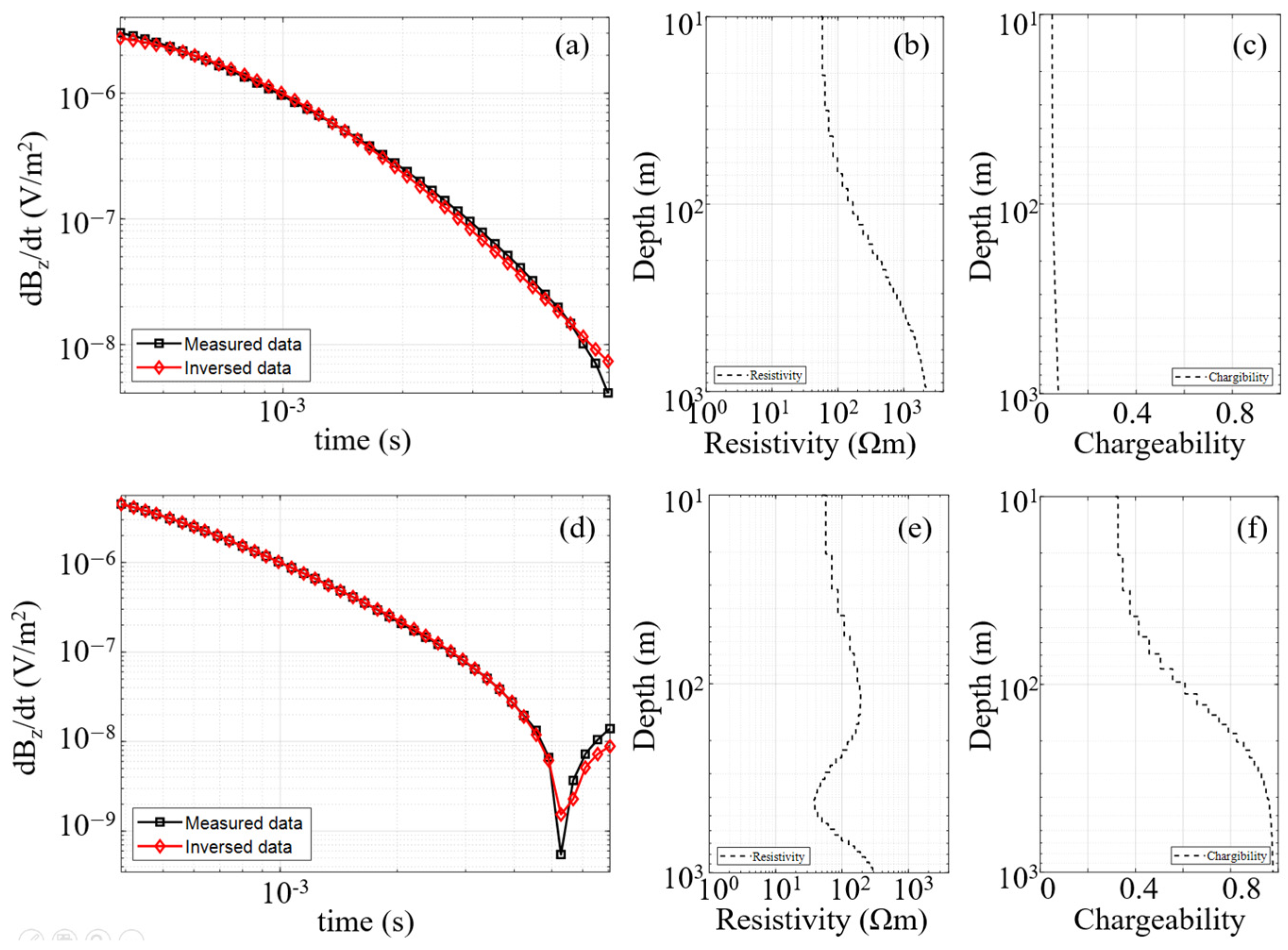
In Figure 7, inversion results for two representative measurement points within the survey area are presented, one of which is significantly affected by the IPE, whereas the other is essentially unaffected by the IPE. Because eddy-current fields and induced polarization effects are two independent physical processes, resistivity and chargeability are two independent parameters. The results in Figure 7 demonstrate that the inversion method is able to clearly distinguish whether the data are affected by the IPE. At the same time, we also note that, during the joint inversion, the sensitivity of chargeability is not exactly the same as that of resistivity. By comparing panels (e) and (f) in Figure 6, it can be observed that for a low-resistivity, high-chargeability zone located at a certain subsurface depth, both resistivity and chargeability undergo rapid changes when the inversion depth reaches the top of the anomaly. However, as the inversion depth increases and exceeds the bottom of the anomalous body, resistivity changes more rapidly than chargeability. At a macroscopic level, this phenomenon manifests as a pronounced high-value shielding effect of chargeability; that is, the chargeability parameter is relatively sensitive to the upper boundary of a high-polarization anomaly, whereas its ability to resolve the lower boundary is comparatively weaker. Based on this characteristic, geological interpretation should generally rely primarily on resistivity results, with chargeability results serving as a supplementary constraint. Chargeability provides additional information that can be used for rock physical property analysis; however, its resolving power is stronger in shallow parts than in deeper parts, particularly with respect to the delineation of the lower boundary of anomalous bodies.

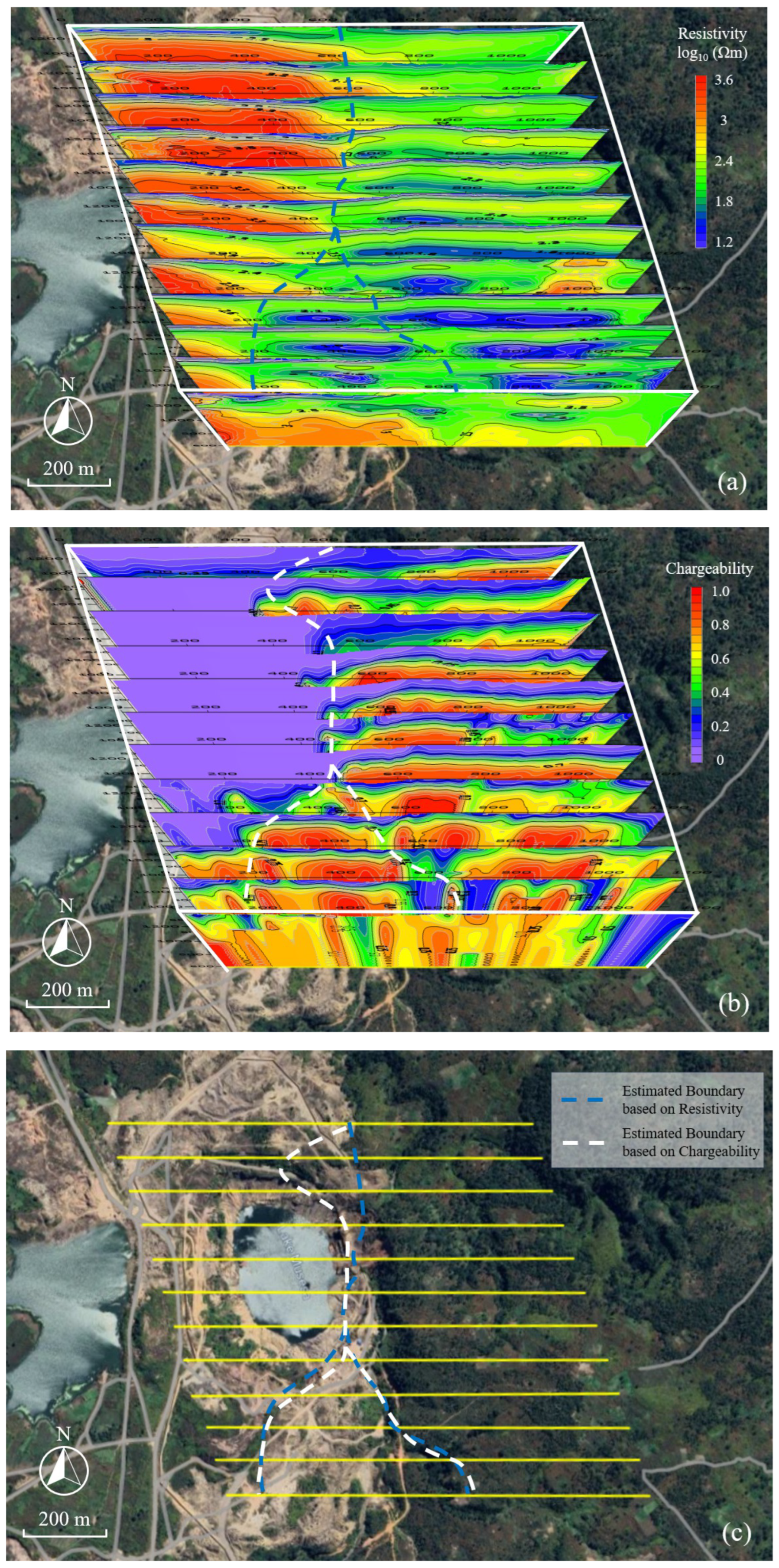
As shown in Figure 8, we placed the inversion profiles on the satellite image, where panel (a) presents the resistivity profiles and panel (b) presents the chargeability profiles. To better highlight macroscopic features, the measurement points were sparsified. From a macroscopic perspective, good continuity of data between adjacent survey lines can be observed, indicating that the system operated in a stable manner during both data acquisition and processing. Existing geological observations indicate that the mining area is located within the Shangoluwe–M’sesa shear zone, where a strike–slip fault with a length of approximately 6.2 km is present and exhibits a nearly vertical attitude. By referring to the satellite imagery and geological map, it can be seen that, taking the fractures on the eastern side of the original pit as an approximate boundary, the deep geological structures on the eastern and western sides show significant contrasts in physical properties. On the western side, the structures are characterized by high resistivity and low chargeability. On the eastern side, resistivity is overall significantly lower than that on the western side, and within the depth range of approximately 200–400 m along several survey lines located relatively to the south, a low-resistivity zone with resistivity generally below 100 Ω·m is observed. Corresponding to this low-resistivity zone, chargeability is markedly elevated, indicating a low-resistivity–high-chargeability characteristic in this area. Further observations show that, in the shallow to middle depths, the boundary between the eastern and western structures is nearly vertical, which is highly consistent with existing geological observations. However, at greater depths, the high-resistivity–low-chargeability structure on the western side appears to extend eastward, exhibiting a tendency to uplift the eastern structure from below. Based on the macroscopic discontinuities in physical properties, inferred geological discontinuity boundaries were delineated on the resistivity and chargeability images, represented by deep blue and white dashed lines, respectively. When these two inferred boundaries are projected onto the satellite map (Figure 8c), both lines reflect the following features. In the northern part of the survey area, the structural boundary is located to the east of the original pit and extends southward along the eastern margin of the pit. To the south of the eastern margin of the pit, a structural bifurcation appears to occur: one branch extends southwestward along the southern margin of the pit, whereas the other branch extends approximately toward the south-southeast. According to the inversion results, the nature of these two branches is different. The branch extending southwestward is similar to the northern branch, and both reflect boundaries of the high-resistivity–low-chargeability zone. In contrast, the branch extending toward the south-southeast appears to indicate the presence of a subsurface fault that truncates the low-resistivity–high-chargeability zone. In addition, it can be observed that the structural boundaries delineated separately from resistivity and chargeability results largely coincide near the orebody and along the two southward-extending branches. However, in the northern part of the pit, the two boundaries do not completely overlap, which is mainly caused by the results from survey line 2. According to the figure, the area enclosed between the two curves is characterized by medium resistivity and low chargeability and is relatively shallow. Previous geological investigations indicate that the undeveloped northern portion of the known No. 3 orebody (oxide orebody) is located precisely in this area, which is inferred to be the cause of this physical property signature. Overall, these macroscopic interpretations show a high degree of consistency with observations from previous ground-based geological investigations. However, the conditions at greater depths require further analysis.

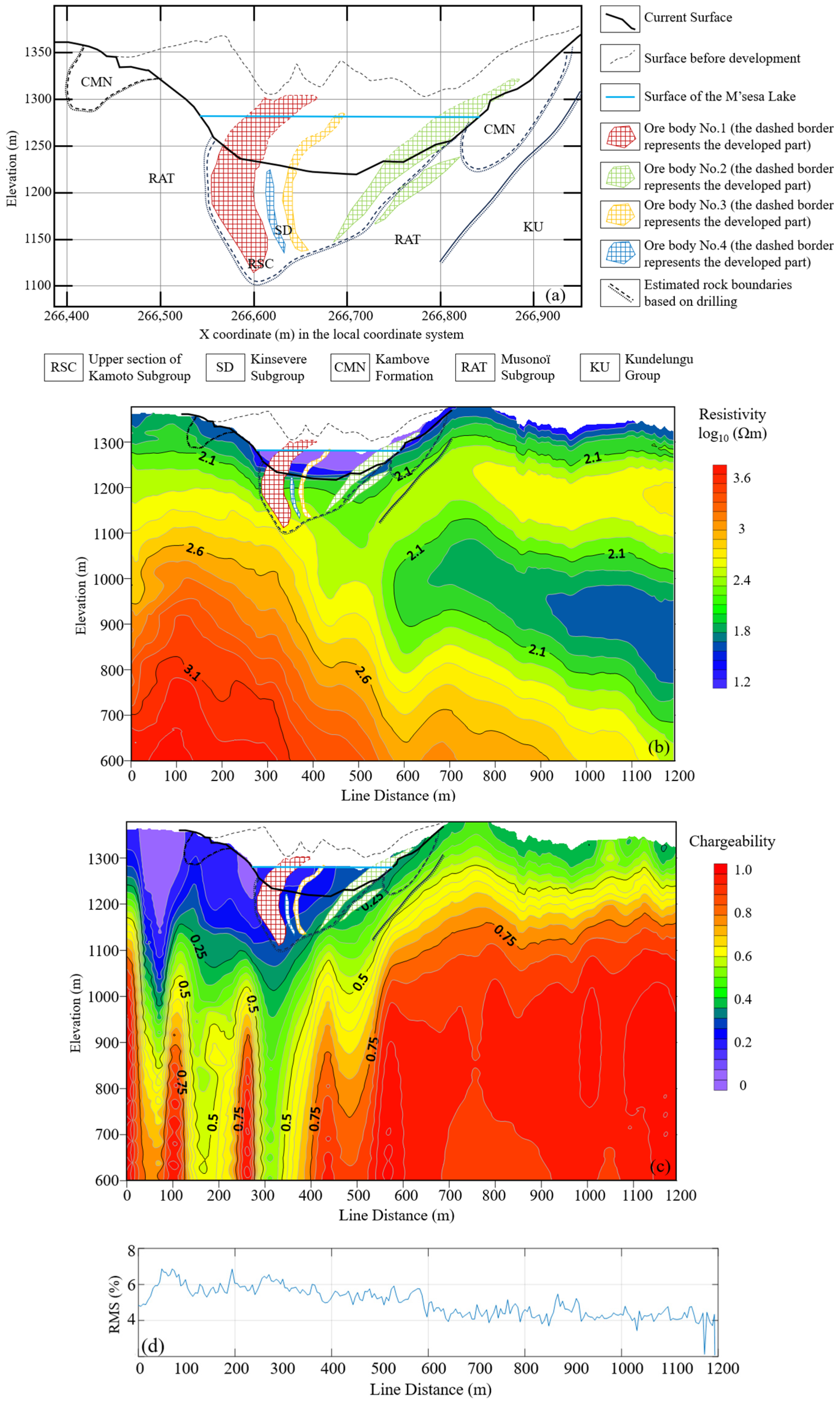
Survey line L4 will be taken as an example for further analysis of the exploration results. Line L4 crosses the M’sesa lake; that is, it passes through the interior of the former mine pit, where relatively abundant prior geological data are available. In Figure 9, panel (a) presents a geological profile constructed based on previous drilling data, with its location indicated in Figure 2; panel (b) shows the resistivity profile of L4, and panel (c) shows the chargeability profile of L4. Panel (d) shows the inversion errors of all the survey points along L4. Overall, the inversion errors of most survey points are less than 6%. For ease of comparison, the exploration profile in panel (a) is superimposed onto panels (b) and (c). Because the length of the existing geological profile is limited, a survey-line distance of 700 m is taken as the boundary in panels (b) and (c). The 0–700 m interval containing the geological profile is first analyzed, followed by an assessment of the mineralization potential along the entire survey line.

Within the 0–700 m interval of line L4, land and lake areas can be distinguished based on topography. On land, the near-surface zone exhibits low resistivity due to the influence of groundwater, whereas the lake area as a whole shows low resistivity because of the mineral-rich water. From the surface downward, the resistivity of the subsurface on the western side increases with depth, forming a high-resistivity zone that also extends eastward with increasing depth. When the geological profile is superimposed on the resistivity profile, it can be observed that the known ore-controlling structures generally lie within the 200 Ω·m contour (corresponding to a logarithmic value of 2.3 in the figure). The No. 1, No. 3, and No. 4 orebodies on the western side all exhibit a tendency to extend eastward at depth, and their orientations show a high degree of consistency with the trend of the boundary of the high-resistivity zone. In addition, within the survey-line distance range of 500–700 m, the boundary between the Musonoï Subgroup (RAT) and the Kundelungu Group (KU), as inferred from previous drilling, also shows good correspondence with the 200 Ω·m resistivity boundary. Next, the chargeability profile is examined. In this area, chargeability is relatively low within the depth range of approximately 100–250 m and gradually increases with depth. Comparison with the exploration profile indicates that the identified orebodies are all located within low-chargeability zones, and the boundaries of these low-chargeability zones spatially correspond well with the boundaries shown in the exploration profile. Analysis of this phenomenon suggests two possible reasons. First, due to the widespread presence of liquid water and near-surface fractures with good connectivity and relatively large apertures, the conditions for generating induced polarization effects are weak. Second, the orebodies identified in this area are mainly oxide orebodies, which inherently have a relatively weak capacity to produce induced polarization effects. Overall, comparison with the exploration profile demonstrates that the spatial distribution patterns of resistivity and chargeability are highly consistent with the available geological information.

In the resistivity profile, we note a low-resistivity zone in the central part of the eastern side of the line. This zone extends westward. In the chargeability profile, this low-resistivity zone (although its lower boundary cannot be precisely delineated from the chargeability image) exhibits relatively high chargeability. This characteristic of low resistivity and high chargeability has drawn our particular attention. From the resistivity profile, it can be observed that there is a certain spatial correlation between the low-resistivity–high-chargeability zone in the deep part and the oxidized orebody area in the shallow part (the area covered by the existing geological profile). In combination with the local geological conditions, the low-resistivity–high-chargeability zone in the deep part on the east side of the profile may provide exploration clues for the subsequent exploration of deep sulfide orebodies. Of course, although the “low-resistivity–high-chargeability” feature is usually taken as a prospecting indicator for sulfide deposits, the earth is a complex system, and there are still other structural factors (such as the downward extension of thrust structures) that can lead to a similar feature. Therefore, further investigation is still needed to determine the actual rock properties of this anomalous area.

Through this exploration work, we can recognize the unique advantages of the semi-airborne electromagnetic method in conducting underground mineral exploration. However, we should also note that this method still has certain limitations. For instance, the high-value shielding effect of the polarization rate inversion results makes it difficult to accurately recognize the induced polarization conditions of the deep structure. To address this issue, besides further optimizing inversion algorithms, the integration of ground-based observation techniques (e.g., ground-induced polarization methods) or the incorporation of deep borehole data (where available) for constrained inversion can enhance exploration performance. Additionally, with the miniaturization of geophysical payloads, such as miniaturized magnetometers and gamma-ray spectrometers, they can also be carried by UAVs. Fusing these detection results with those obtained using electromagnetic methods that can penetrate the earth will facilitate a more accurate estimation of underground structures.

4. Conclusions

In recent years, unmanned aerial vehicles have increasingly been used as carrying platforms for Earth observation. In a large number of Earth observation studies, UAVs equipped with optical, microwave, and other types of sensors have enabled high-resolution observations of targets above the ground surface. With the advancement of geophysical theory and methods, technological innovations have transformed instrument configurations, allowing conventional civilian UAVs to serve as carrying platforms for deep and high-resolution exploration of subsurface targets. Accordingly, we developed the DROEM system based on the SATEM method and conducted a survey in the Kambove area of the Democratic Republic of the Congo. The airborne survey was completed within 3 h, during which resistivity and chargeability information of the survey area was successfully extracted. The results clearly delineate the depth distribution of the Shangoluwe–M’sesa compressional fault and reveal a low-resistivity–high-chargeability zone at depth on the eastern side of the fault, providing clues for the exploration of deep deposits. This study will be of significant importance for accelerating the promotion and application of UAV-based semi-airborne electromagnetic exploration technologies.

References

1. Nabighian, M.N.; Corbett, J.D. Electromagnetic Methods in Applied Geophysics: Volume 1, Theory; Society of Exploration Geophysicists: Houston, TX, USA, 1987; ISBN 978-1-56080-263-1. [Google Scholar]
2. Auken, E.; Christiansen, A.V.; Westergaard, J.H.; Kirkegaard, C.; Foged, N.; Viezzoli, A. An Integrated Processing Scheme for High-Resolution Airborne Electromagnetic Surveys, the SkyTEM System. Explor. Geophys. 2009, 40, 184–192. [Google Scholar] [CrossRef]
3. Studinger, M.; Bell, R.; Frearson, N. Comparison of AIRGrav and GT-1A Airborne Gravimeters for Research Applications. Geophysics 2008, 73, I51–I61. [Google Scholar] [CrossRef]
4. Sanada, Y.; Torii, T. Aerial Radiation Monitoring around the Fukushima Dai-Ichi Nuclear Power Plant Using an Unmanned Helicopter. J. Environ. Radioact. 2015, 139, 294–299. [Google Scholar] [CrossRef]
5. Niethammer, U.; James, M.R.; Rothmund, S.; Travelletti, J.; Joswig, M. UAV-Based Remote Sensing of the Super-Sauze Landslide: Evaluation and Results. Eng. Geol. 2012, 128, 2–11. [Google Scholar] [CrossRef]
6. Liu, S.; Hu, X.; Guo, N.; Cai, H.; Zhang, H.; Li, Y. Overview on UAV Aeromagnetic Survey Technology. Geomat. Inf. Sci. Wuhan Univ. 2023, 48, 823–840. [Google Scholar] [CrossRef]
7. Yanushevsky, R. Guidance of Unmanned Aerial Vehicles; CRC Press: Boca Raton, FL, USA, 2011; ISBN 978-0-429-10989-8. [Google Scholar]
8. Hatch, M. Environmental Geophysics. Preview 2016, 2016, 31–32. [Google Scholar] [CrossRef]
9. Zheng, Y.; Li, S.; Xing, K.; Zhang, X. Unmanned Aerial Vehicles for Magnetic Surveys: A Review on Platform Selection and Interference Suppression. Drones 2021, 5, 93. [Google Scholar] [CrossRef]
10. Zhdanov, M.S. Inverse Theory and Applications in Geophysics; Elsevier: Amsterdam, The Netherlands, 2015; ISBN 978-0-444-62674-5. [Google Scholar]
11. Annan, A.P.; Lookwood, R. An Application of Airborne Geotem* in Australian Conditions. Explor. Geophys. 1991, 22, 5–12. [Google Scholar] [CrossRef]
12. Smith, R.S.; Annan, A.P.; Lemieux, J.; Pedersen, R.N. Application of a Modified GEOTEM System to Reconnaissance Exploration for Kimberlites in the Point Lake Area, NWT, Canada. Geophysics 1996, 61, 82–92. [Google Scholar] [CrossRef]
13. Witherly, K.; Irvine, R.; Morrison, E. The Geotech VTEM Time Domain Helicopter Em System. ASEG Ext. Abstr. 2004, 2004, 1–4. [Google Scholar] [CrossRef]
14. Mogi, T.; Kusunoki, K.; Kaieda, H.; Ito, H.; Jomori, A.; Jomori, N.; Yuuki, Y. Grounded Electrical-Source Airborne Transient Electromagnetic (GREATEM) Survey of Mount Bandai, North-Eastern Japan. Explor. Geophys. 2009, 40, 1–7. [Google Scholar] [CrossRef]
15. Ji, Y.J.; Wang, Y.; Xu, J.; Zhou, F.D.; Li, S.Y.; Zhao, Y.P.; Lin, J. Development and application of the grounded long wire source airborne electromagnetic exploration system based on an unmanned airship. Chin. J. Geophys. 2013, 56, 3640–3650. [Google Scholar] [CrossRef]
16. Smirnova, M.V.; Becken, M.; Nittinger, C.; Yogeshwar, P.; Mörbe, W.; Rochlitz, R.; Steuer, A.; Costabel, S.; Smirnov, M.Y.; the DESMEX Working Group. A Novel Semiairborne Frequency-Domain Controlled-Source Electromagnetic System: Three-Dimensional Inversion of Semiairborne Data from the Flight Experiment over an Ancient Mining Area near Schleiz, Germany. Geophysics 2019, 84, E281–E292. [Google Scholar] [CrossRef]
17. Wu, X.; Rao, L.-T.; Luan, X.-D.; Shi, J.-J.; Wang, Y.-B. Design and Development of a Semiairborne Transient Electromagnetic System. Geophysics 2024, 89, E255–E266. [Google Scholar] [CrossRef]
18. Wu, X.; Xue, G.; Fang, G.; Li, X.; Ji, Y. The Development and Applications of the Semi-Airborne Electromagnetic System in China. IEEE Access 2019, 7, 104956–104966. [Google Scholar] [CrossRef]
19. Macnae, J. Quantifying Airborne Induced Polarization Effects in Helicopter Time Domain Electromagnetics. J. Appl. Geophys. 2016, 135, 495–502. [Google Scholar] [CrossRef]
20. Mörbe, W.; Yogeshwar, P.; Tezkan, B.; Kotowski, P.; Thiede, A.; Steuer, A.; Rochlitz, R.; Günther, T.; Brauch, K.; Becken, M. Large-Scale 3D Inversion of Semi-Airborne Electromagnetic Data—Topography and Induced Polarization Effects in a Graphite Exploration Scenario. Geophysics 2024, 89, B339–B352. [Google Scholar] [CrossRef]
21. Pelton, W.H.; Ward, S.H.; Hallof, P.G.; Sill, W.R.; Nelson, P.H. Mineral Discrimination and Removal of Inductive Coupling with Multifrequency IP. Geophysics 1978, 43, 588–609. [Google Scholar] [CrossRef]
22. Wong, J. An Electrochemical Model of the Induced-Polarization Phenomenon in Disseminated Sulfide Ores. Geophysics 1979, 44, 1245–1265. [Google Scholar] [CrossRef]
23. Hine, K.; Macnae, J. Comparing Induced Polarization Responses from Airborne Inductive and Galvanic Ground Systems: Lewis Ponds, New South Wales. Geophysics 2016, 81, B179–B188. [Google Scholar] [CrossRef]
24. Viezzoli, A.; Kaminski, V.; Fiandaca, G. Modeling Induced Polarization Effects in Helicopter Time Domain Electromagnetic Data: Synthetic Case Studies. Geophysics 2017, 82, E31–E50. [Google Scholar] [CrossRef]
25. Mir, R.; Perrouty, S.; Astic, T.; Bérubé, C.L.; Smith, R.S. Structural Complexity Inferred from Anisotropic Resistivity: Example from Airborne EM and Compilation of Historical Resistivity/Induced Polarization Data from the Gold-Rich Canadian Malartic District, Québec, Canada. Geophysics 2019, 84, B153–B167. [Google Scholar] [CrossRef]
26. Wu, X.; Xue, G.-Q.; Liu, Y.; Wang, Y.-B.; Zhang, J.-E.; Chen, W.-Y.; He, L.-F.; Zhao, Y.-G. Brownfields Exploration Using Semi-Airborne Transient Electromagnetic Surveys at the Giant Bayan Obo REE-Nb-Fe Deposit, Inner Mongolia, China. Ore Geol. Rev. 2025, 181, 106610. [Google Scholar] [CrossRef]
27. Chen, P.P.; Yang, Y.Q.; Dai, J.C.; Guo, Q.L.; Chen, T.H. Ore-controlling factor and exploration prospect of KZ Cu-Co deposit in Kambove area, Haut-katanga Province, DRCongo. Miner. Resour. Geol. 2023, 37, 1145–1153. [Google Scholar] [CrossRef]
28. Li, C.B.; Mao, F.L.; Zhang, Y.; Zhang, X.S.; Pang, X.Y.; Zhan, C.F. Metallogenesis and Ore Deposit Genesis of the Central African Katanga Copper-Cobalt Belt: A Case Study of the Kamoya Deposit in the Democratic Republic of Congo (DRC). Geol. Explor. 2025, 61, 655–666. [Google Scholar]
29. Cailteux, J.L.H.; Kampunzu, A.B.; Lerouge, C.; Kaputo, A.K.; Milesi, J.P. Genesis of Sediment-Hosted Stratiform Copper–Cobalt Deposits, Central African Copperbelt. J. Afr. Earth Sci. 2005, 42, 134–158. [Google Scholar] [CrossRef]
30. Master, S. Stratabound Sediment-Hosted Cu–Co Deposits (with Special Reference to the Central African Copperbelt). In Encyclopedia of Geology; Selly, R.C., Cocks, L.R.M., Plimer, I.R., Eds.; Elsevier: Amsterdam, The Netherlands, 2021; pp. 899–913. ISBN 978-0-08-102909-1. [Google Scholar]
31. Torres, J.; Muchez, P. Fluid Evolution and Cu-Co Ore-Forming Processes in the Katanga Copperbelt (DR Congo)—Insights from Laser Ablation-Inductively Coupled Plasma-Mass Spectrometry Analyses of Fluid Inclusions. Econ. Geol. 2025, 120, 61–85. [Google Scholar] [CrossRef]
32. Unrug, R. Mineralization Controls and Source of Metals in the Lufilian Fold Belt, Shaba (Zaire), Zambia, and Angola. Econ. Geol. 1988, 83, 1247–1258. [Google Scholar] [CrossRef]
33. Batumike, M.J.; Cailteux, J.L.H.; Kampunzu, A.B. Lithostratigraphy, Basin Development, Base Metal Deposits, and Regional Correlations of the Neoproterozoic Nguba and Kundelungu Rock Successions, Central African Copperbelt. Gondwana Res. 2007, 11, 432–447. [Google Scholar] [CrossRef]
34. Cailteux, J.L.H.; De Putter, T. The Neoproterozoic Katanga Supergroup (D. R. Congo): State-of-the-Art and Revisions of the Lithostratigraphy, Sedimentary Basin and Geodynamic Evolution. J. Afr. Earth Sci. 2019, 150, 522–531. [Google Scholar] [CrossRef]
35. John, T.; Schenk, V.; Mezger, K.; Tembo, F. Timing and PT Evolution of Whiteschist Metamorphism in the Lufilian Arc–Zambezi Belt Orogen (Zambia): Implications for the Assembly of Gondwana. J. Geol. 2004, 112, 71–90. [Google Scholar] [CrossRef]
36. Mambwe, P.; Swennen, R.; Cailteux, J.; Mumba, C.; Dewaele, S.; Muchez, P. Review of the Origin of Breccias and Their Resource Potential in the Central Africa Copperbelt. Ore Geol. Rev. 2023, 156, 105389. [Google Scholar] [CrossRef]
37. Kampunzu, A.B.; Cailteux, J.L.H.; Kamona, A.F.; Intiomale, M.M.; Melcher, F. Sediment-Hosted Zn–Pb–Cu Deposits in the Central African Copperbelt. Ore Geol. Rev. 2009, 35, 263–297. [Google Scholar] [CrossRef]
38. Wendorff, M. Tectonosedimentary Expressions of the Evolution of the Fungurume Foreland Basin in the Lufilian Arc, Neoproterozoic–Lower Palaeozoic, Central Africa. Geol. Soc. Lond. Spec. Publ. 2011, 357, 69–83. [Google Scholar] [CrossRef]
39. Kipata, M.L.; Delvaux, D.; Sebagenzi, M.N.; Cailteux, J.; Sintubin, M. Brittle Tectonic and Stress Field Evolution in the Pan-African Lufilian Arc and Its Foreland (Katanga, DRC): From Orogenic Compression to Extensional Collapse, Transpressional Inversion and Transition to Rifting. Geol. Belg. 2013, 16, 001–017. [Google Scholar]
40. Mambwe, P.; Kipata, L.; Chabu, M.; Muchez, P.; Lubala, T.; Jébrak, M.; Delvaux, D. Sedimentology of the Shangoluwe Breccias and Timing of the Cu Mineralisation (Katanga Supergroup, D.R. of Congo). J. Afr. Earth Sci. 2017, 132, 1–15. [Google Scholar] [CrossRef]
41. Cailteux, J. Lithostratigraphy of the Neoproterozoic Shaba-Type (Zaire) Roan Supergroup and Metallogenesis of Associated Stratiform Mineralization. J. Afr. Earth Sci. 1994, 19, 279–301. [Google Scholar] [CrossRef]
42. Mambwe, P.; Shengo, M.; Kidyanyama, T.; Muchez, P.; Chabu, M. Geometallurgy of Cobalt Black Ores in the Katanga Copperbelt (Ruashi Cu-Co Deposit): A New Proposal for Enhancing Cobalt Recovery. Minerals 2022, 12, 295. [Google Scholar] [CrossRef]
43. Macnae, J.; Lamontagne, Y.; West, G.F. Noise processing techniques for time Domain EM systems. Geophysics 1984, 49, 934–948. [Google Scholar] [CrossRef]
44. Qi, W.J.; Yu, L.; Tang, X.; Wu, J.Y.; Zhang, Y.; He, Z.Q. Multi-objective optimization of a hydrogen-fueled PEMFC with multi wavy channels via machine learning and CFD simulation. Int. J. Hydrogen Energy 2026, 199, 152748. [Google Scholar] [CrossRef]
45. Qi, W.J.; Yang, J.X.; Zhang, Z.G.; Wu, J.Y.; Lan, P.; Xiang, S.L. Investigation on thermal management of cylindrical lithium-ion batteries based on interwound cooling belt structure. Energy Convers. Manag. 2025, 340, 119962. [Google Scholar] [CrossRef]
46. Munkholm, M.S. Motion-Induced Noise from Vibration of a Moving TEM Detector Coil: Characterization and Suppression. J. Appl. Geophys. 1997, 37, 21–29. [Google Scholar] [CrossRef]
47. FeimaRobotics-E3000. Available online: https://astrowind.vercel.app/products/multirotor/e3000 (accessed on 29 January 2026).
48. Bednar, J.B.; Watt, T.L. Alpha-Trimmed Means and Their Relationship to Median Filters. IEEE Trans. Acoust. Speech Signal Process. 1984, 32, 145–153. [Google Scholar] [CrossRef]
49. Wu, X.; Xue, G.; He, Y.; Xue, J. Removal of Multisource Noise in Airborne Electromagnetic Data Based on Deep Learning. Geophysics 2020, 85, B207–B222. [Google Scholar] [CrossRef]
50. Vincent, P.; Larochelle, H.; Bengio, Y.; Manzagol, P.-A. Extracting and Composing Robust Features with Denoising Autoencoders. In Proceedings of the 25th International Conference on Machine Learning (ICML’08); ACM Press: Helsinki, Finland, 2008; pp. 1096–1103. [Google Scholar]
51. Wu, X.; Xue, G.; Zhao, Y.; Lv, P.; Zhou, Z.; Shi, J. A Deep Learning Estimation of the Earth Resistivity Model for the Airborne Transient Electromagnetic Observation. J. Geophys. Res. Solid Earth 2022, 127, e2021JB023185. [Google Scholar] [CrossRef]
52. Pisa, I.; Morell, A.; Vicario, J.L.; Vilanova, R. Denoising Autoencoders and LSTM-Based Artificial Neural Networks Data Processing for Its Application to Internal Model Control in Industrial Environments—The Wastewater Treatment Plant Control Case. Sensors 2020, 20, 3743. [Google Scholar] [CrossRef]
53. Mörbe, W.; Yogeshwar, P.; Tezkan, B.; Hanstein, T. Deep Exploration Using Long-offset Transient Electromagnetics: Interpretation of Field Data in Time and Frequency Domain. Geophys. Prospect. 2020, 68, 1980–1998. [Google Scholar] [CrossRef]
54. Qi, Y.; Ahmed, A.S.; Revil, A.; Ghorbani, A.; Abdulsamad, F.; Florsch, N.; Bonnenfant, J. Induced Polarization Response of Porous Media with Metallic Particles—Part 7: Detection and Quantification of Buried Slag Heaps. Geophysics 2018, 83, E277–E291. [Google Scholar] [CrossRef]
55. Man, K.F.; Yin, C.C.; Liu, Y.H.; Sun, S.Y.; Xiong, B. 3D Inversion of Time-Domain Airborne EM Data for IP Parameters. Chin. J. Geophys. 2023, 66, 1269–1280. [Google Scholar] [CrossRef]
56. Kratzer, T.; Macnae, J.C. Induced polarization in airborne EM. Geophysics 2012, 77, E317–E327. [Google Scholar] [CrossRef]
57. Stolz, E.; Macnae, J. Evaluating EM waveforms by singular-value decomposition of exponential basis functions. Geophysics 1998, 63, 64–74. [Google Scholar] [CrossRef]
58. Gill, P.E.; Murray, W. Algorithms for the Solution of the Nonlinear Least-Squares Problem. SIAM J. Numer. Anal. 1978, 15, 977–992. [Google Scholar] [CrossRef]
Figure 2. The design of the transmitting antenna (light blue line) and the survey line (yellow line).
Drones 10 00293 g002
Figure 3. Field device layout method and detection scenarios.
Drones 10 00293 g003
Figure 4. The UAVs used for detection and the actual deployment method.
Drones 10 00293 g004
Figure 6. The raw data was processed by the flow-based processing method (TPF) and DAE. Panels (b,d) show the processing results of panels (a,c) respectively. Compared with panel (b), the data in panel (d) is significantly affected by the IPE.
Drones 10 00293 g006
Figure 7. The inversion results of two typical measurement points, where (ac) belong to a measurement point that is basically not affected by the IPE, while (df) belong to a measurement point that is significantly affected by the IPE.
Drones 10 00293 g007
Figure 8. The inversion results of each survey line (yellow line) within the survey area are arranged in spatial order, where (a) represents the resistivity results, (b) the chargeability results, and (c) the inferred geological boundary derived from the inversion results.
Drones 10 00293 g008
Figure 9. The geological profile (a) of the existing exploration line in the west section of survey line 4 and the inversion results of survey line 4, where (b) is the resistivity result, (c) is the chargeability result and (d) is the error of all survey points along survey line 4.
Drones 10 00293 g009
Disclaimer/Publisher’s Note: The statements, opinions and data contained in all publications are solely those of the individual author(s) and contributor(s) and not of MDPI and/or the editor(s). MDPI and/or the editor(s) disclaim responsibility for any injury to people or property resulting from any ideas, methods, instructions or products referred to in the content.