Article

Efficient Multi-Fidelity Surrogate Modeling for UAV Aerodynamic Analysis via Active Transfer Learning

School of Aerospace Engineering, Beijing Institute of Technology, Beijing 100081, China
*
Author to whom correspondence should be addressed.
Drones 2026, 10(4), 290; https://doi.org/10.3390/drones10040290
Submission received: 24 February 2026 / Revised: 26 March 2026 / Accepted: 27 March 2026 / Published: 16 April 2026
(This article belongs to the Section Drone Design and Development)

Highlights

What are the main fundings?
  • An active transfer learning-based multi-fidelity surrogate modeling framework is developed to achieve high-accuracy UAV aerodynamic prediction under severely limited high-fidelity data.
  • The proposed GPR-assisted active sampling and composite transfer loss significantly improve prediction accuracy, robustness, and convergence compared with conventional multi-fidelity and hierarchical Kriging approaches.
What are the implications of the main findings?
  • The proposed framework enables reliable UAV aerodynamic surrogate modeling with only a small number of high-fidelity evaluations, substantially reducing the computational cost during early-stage design.
  • The method provides a practical and scalable tool for aerodynamic analysis and the optimization of UAV airfoils, supporting efficient engineering-driven design exploration.

Abstract

During the design and optimization phase of unmanned aerial vehicles (UAVs), high-fidelity aerodynamic analysis methods often come with high computational costs, significantly restricting the efficiency of design exploration. To address this challenge, a multi-fidelity surrogate modeling method based on active transfer learning is proposed. The method leverages transfer learning to capture implicit correlations among multi-fidelity analysis models, while an active learning-based adaptive sampling strategy is introduced to reduce the computational cost during model construction. To further reduce the computational burden, a Gaussian process regression-assisted active learning criterion is formulated to efficiently select high-value samples and a model updating strategy is designed to ensure feature consistency, accelerate convergence, and enhance the robustness during the transfer process. Numerical benchmarks, NACA 0012 airfoil aerodynamic analysis and UAV with strut-braced wing aerodynamic analysis cases, are conducted to validate the proposed approach. The results demonstrate that the proposed method achieves a higher accuracy under small-sample conditions compared with traditional approaches.

1. Introduction

During the conceptual design and optimization phase of UAVs, high-fidelity (HF) analyses, such as Reynolds-averaged Navier–Stokes (RANS)-based aerodynamic simulations, are computationally expensive and time-consuming, which has made model construction efficiency a persistent bottleneck [1]. Therefore, surrogate modeling, which replaces repeated HF evaluations with computationally inexpensive predictors, has become a common enabling tool for large-scale parameter exploration and multidisciplinary design optimization (MDO) [2,3]. In recent years, surrogate-assisted analysis workflows have increasingly been used in UAV studies to accelerate conceptual design and robust optimization [4,5]. At the aerodynamic analysis level, physics-informed surrogate models have emerged as a recent research trend. By embedding governing equations, boundary conditions, or physical priors into the learning process, such methods improve physical consistency and, to some extent, alleviate the poor generalization of purely data-driven models under small-sample conditions [6,7]. However, these methods still face difficulties in training, sensitivity to parameter settings, and limited engineering applicability in the presence of complex flows, strong nonlinear coupling, and high-dimensional design spaces. Moreover, most existing studies are still focused on airfoil-level problems, making them difficult to apply directly to the aerodynamic analysis of complex UAV configurations.
For aerodynamic analysis of complex UAVs, multi-fidelity surrogate models have become a major research focus [2,8,9]. Their core idea is to exploit the complementary characteristics of low-fidelity (LF) and high-fidelity models: LF tools, such as panel methods, vortex lattice methods (VLM), and simplified structural solvers, are computationally efficient but biased, whereas HF solvers provide more reliable predictions at a much higher computational cost. By learning cross-fidelity coupling (or discrepancy) relationships and fusing multi-source information, multi-fidelity surrogate models aim to achieve an effective trade-off between accuracy and cost.
Classical forms such as co-Kriging [10] and hierarchical Kriging [11] have been widely adopted; for example, a co-Kriging model combined with expected-improvement (EI)-driven infill sampling has been used for aerodynamic performance modeling [12]. Notably, recent UAV-oriented studies have also shown that, under complex aerodynamic conditions, maintaining a consistently high prediction accuracy often still requires a considerable number of HF samples (e.g., on the order of several hundred HF evaluations), which highlights the practical difficulty of HF-scarce scenarios [12].
Furthermore, multi-fidelity neural networks have recently attracted broad attention. Zhang et al. investigated aerodynamic shape optimization using a multi-fidelity deep neural network and improved the expressive capability of cross-fidelity mappings in high-dimensional settings; however, because the LF and HF data were mainly generated from coarse and fine meshes of the same CFD model, the issues of local LF distortion and negative transfer were not fully addressed [13]. Meliani et al. combined multi-fidelity surrogates with Bayesian optimization and infill sampling, thereby reducing the cost of HF evaluations during optimization; however, this class of methods primarily targets low-cost optimal solution search rather than globally reliable modeling under extremely scarce HF samples [14]. Aye et al. further introduced multi-objective infill sampling into XFoil–CFD multi-fidelity airfoil optimization, improving sample efficiency in surrogate-assisted optimization; however, their sampling criterion still mainly revolves around optimization performance and does not explicitly assess the reliability of cross-fidelity knowledge transfer [15]. Yang et al. extended multi-fidelity data-driven optimization to more complex wing-level problems, enhancing the expressive power of surrogates in geometrically complex scenarios [16]. Overall, existing studies have improved aerodynamic modeling efficiency from the perspectives of multi-fidelity deep modeling, adaptive optimization-oriented sampling, and surrogate expressiveness for complex geometries. Nevertheless, for UAV scenarios characterized by extremely scarce HF samples, spatially nonuniform LF reliability, and the need to balance sampling efficiency with transfer reliability, a unified and robust methodological framework is still lacking.
Transfer learning provides a systematic strategy for alleviating HF data scarcity by reusing knowledge learned from a related source task, usually an LF task, to improve prediction in the HF target task. By introducing transferable prior information from LF data, the target surrogate can achieve lower prediction bias and better robustness under limited HF supervision [17]. Recent multi-fidelity studies have shown that cross-fidelity information fusion is an effective way to enhance predictive capability in sparse-data settings [18]. In transfer-learning-based surrogate modeling, representative approaches include input-space transformation methods for reducing distribution mismatch between source and target tasks and transfer risk estimation methods for suppressing negative transfer. However, despite these advances, many existing workflows still require a non-negligible number of initial HF labels to stabilize or anchor the target model, which restricts their usefulness in UAV design problems with severely limited HF evaluation budgets.
To further reduce the demand for HF samples, active transfer learning (ATL) combines transfer learning with active sampling so that information gain can be maximized through automated data acquisition under a strictly limited labeling budget [19,20]. Existing active learning studies in aerodynamic optimization have mainly focused on multi-fidelity infill sampling, adaptive sampling for neural network surrogates, and design space refinement. Meliani et al. improved HF sample efficiency in airfoil optimization by combining multi-fidelity surrogates, Bayesian optimization, and infill sampling, but their method is more oriented toward low-cost optimization than toward globally reliable modeling under HF-scarce conditions [14]. Ghazi et al. used a Gaussian process and an acquisition function to select training samples for neural network surrogates, showing that active learning can also serve the construction of neural network surrogates; however, their study did not explicitly address transfer reliability in multi-fidelity settings [21]. Liu et al. further applied active learning to design space refinement and improved the efficiency of supercritical airfoil optimization, but their focus was on the compression and searching of high-performance regions rather than on robust knowledge utilization under local LF distortion [22]. Therefore, for UAV aerodynamic analysis problems characterized by extremely scarce HF samples and spatially varying LF reliability, it remains necessary to develop an ATL-based multi-fidelity surrogate modeling method that can simultaneously balance sample selection efficiency and cross-fidelity transfer robustness.
In such settings, an active-learning-based sampling strategy must not only identify samples that are informative for the target surrogate model but also prioritize those that are beneficial for reliable transfer, typically requiring a balance among representativeness, diversity, and uncertainty [23,24]. In recent years, several engineering studies have extended active sampling to multi-fidelity settings by explicitly considering the cost–accuracy trade-off across different fidelity levels [25]. For example, some strategies decouple the selection of the next sampling location from the choice of fidelity level and introduce information-theoretic measures, such as the Jensen–Shannon divergence (JSD), to quantify cross-fidelity accuracy; however, candidate locations are still mainly determined by the highest-fidelity surrogate model. More importantly, these methods mostly focus on rapidly approaching locally high-performance regions during optimization and pay less explicit attention to the reliability of cross-fidelity knowledge transfer. As a result, when HF samples are extremely scarce and LF information is not globally reliable across the design space, relying solely on conventional active learning strategies remains insufficient to guarantee the global accuracy and transfer stability of the surrogate model.
It is also necessary to distinguish the present work from other related paradigms. Multi-fidelity Bayesian optimization (MFBO), which is built upon Bayesian optimization (BO), primarily aims to locate the optimum at the lowest possible cost by adaptively deciding where and at which fidelity level to evaluate, and it typically does not target maintaining a globally high-accuracy surrogate model in regions irrelevant to optimization [26]. In addition, data-intensive deep surrogate modeling approaches—for example, those trained on large-scale computational fluid dynamics (CFD) databases using convolutional autoencoders (CAEs) and deep neural networks (DNNs)—have demonstrated a strong simulation replacement capability (e.g., for velocity and turbulent kinetic energy (TKE) fields), but such methods usually depend on large volumes of HF data and non-negligible training costs [27]. Finally, compared with more expressive probabilistic surrogate models such as deep Gaussian process compositions [28], the present work emphasizes a modeling workflow that remains reliable and interpretable under extremely limited data.
Motivated by the above research gaps, this paper proposes an ATL-based multi-fidelity surrogate modeling framework for UAV-related problems, with a particular emphasis on reliable transfer under a limited HF budget. Unlike studies that implicitly assume uniformly reliable LF information, the proposed framework explicitly introduces a transfer credibility mechanism into the sampling decision to mitigate negative transfer and preferentially select samples that can simultaneously (i) reduce target domain uncertainty, (ii) improve cross-fidelity alignment. The main contributions of this work are summarized as follows:
1.
An ATL-based multi-fidelity surrogate modeling framework is proposed, which couples active sampling with iterative model optimization so as to achieve coordinated data acquisition and model improvement under a limited HF budget.
2.
A Gaussian process regression (GPR)-assisted active sampling strategy is proposed, which combines performance information with feasibility information, introduces transfer credibility evaluation, and selects new samples by balancing target accuracy improvement against transfer reliability.
3.
A transfer loss function is proposed that jointly considers prediction accuracy, structural consistency, and domain confusion constraints, thereby promoting the inheritance of transferable features while reducing overfitting and the risk of negative transfer.
The remainder of this paper is organized as follows. Section 2 describes the overall framework and workflow of the proposed method. Section 3 presents the Gaussian process regression-based active sampling strategy and transfer credibility assessment method. Section 4 introduces the transfer loss function developed for multi-fidelity knowledge transfer. Section 5 verifies the effectiveness of the proposed method through numerical case studies. Finally, Section 7 concludes the paper and outlines directions for future work.

2. Active Transfer Learning Framework for Multi-Fidelity UAV Surrogate Modeling

During the aerodynamic analysis and design optimization of UAVs, obtaining accurate surrogate models under limited computational budgets is a key factor for the efficient exploration of the design space. Traditional multi-fidelity surrogate modeling methods often struggle to maintain prediction reliability when high-fidelity data is scarce especially in the early stages of UAV design and in rapid iteration scenarios. To tackle this challenge, this section proposes a multi-fidelity surrogate modeling framework based on active transfer learning (ATL) specifically for drone-related engineering applications. This framework combines transfer learning mechanisms with active sampling loops, enabling continuous interaction between surrogate model updating and data acquisition. By coordinating low-fidelity and high-fidelity models within a unified workflow, the framework gradually improves prediction accuracy while minimizing the reliance on costly high-fidelity evaluations.
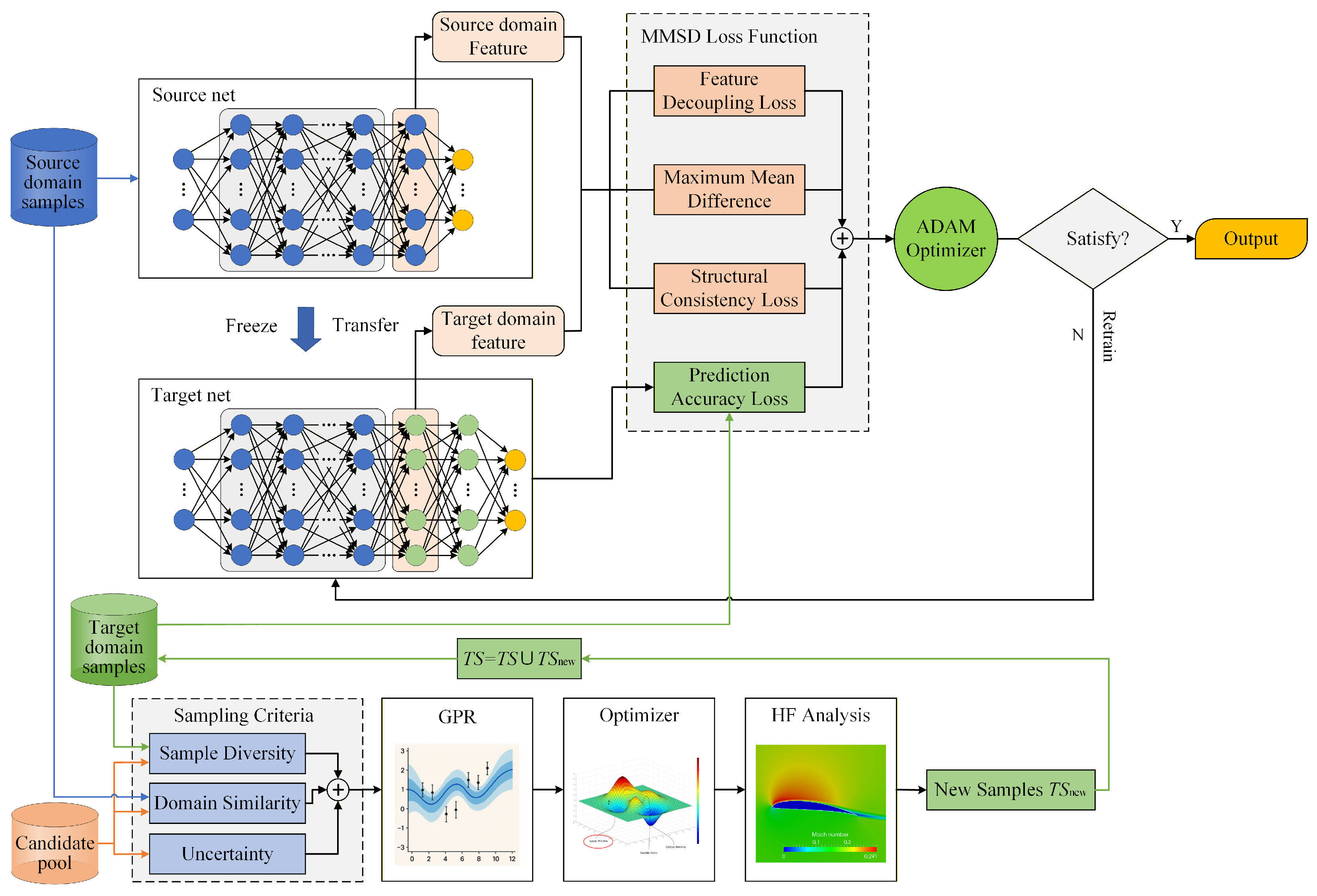
To address the problem of constructing multi-fidelity surrogate models, this study proposes a transfer learning-based surrogate modeling framework assisted by GPR [29] and active sampling; the framework is presented in Figure 1.
The proposed framework adopts a pre-training–fine-tuning paradigm [30] to train the target domain network. The training pipeline comprises the following components:
(1)
Source Domain pre-training
Sample m design points within the domain using Latin Hypercube Sampling [31] (LHS) and generate low-fidelity samples with the low-fidelity analysis model. The LHS method is a space-filling design method that partitions the range of each design variable into N equiprobable strata and enforces that, in every dimension, each stratum is sampled exactly once. This stratified construction typically yields more uniform coverage of the d-dimensional design space than simple random sampling for the same sample sizes.
x j ( i )   =   a j + π j ( i ) u i j N   ( b j a j ) , u i j U ( 0 , 1 ) ,
where x j [ a j , b j ] , π j ( · ) denotes a random permutation of { 1 , , N } , i = 1 , , N , and j = 1 , , d .
Normalize the resulting source domain dataset and split it into training, validation, and test sets. In the practical UAV case study, we apply z-score normalization to each feature to mitigate scale discrepancies among heterogeneous variables and improve numerical stability during model training. Z-score normalization rescales each feature to have zero mean and unit variance, improving numerical stability when features have different physical scales. In practice, the mean μ ( ) and standard deviation σ ( ) are computed from the training set and then applied to validation and test sets to avoid data leakage.
X N ( s ) = X ( s ) μ ( X ( s ) ) σ ( X ( s ) ) , Y N ( s ) = Y ( s ) μ ( Y ( s ) ) σ ( Y ( s ) ) .
where X ( s ) and Y ( s ) denote the source domain design variables and objective functions, respectively, while X N ( s ) and Y N ( s ) represent the normalized source domain design variables and objective functions.
Train the source domain network on the normalized training set, use the validation set to accelerate convergence, and report accuracy on the test set.
(2)
Target Domain Sample Selection
Employ the proposed active learning strategy (Section 3.1) to pick n samp samples at each of i t e r iterations, yielding a total of n = n samp × i t e r target samples. A candidate pool is constructed using Latin Hypercube Sampling (LHS) to guarantee uniform coverage of the design space. The number of candidates is set as N samp = 50   n hf , where n hf represents the maximum number of high-fidelity analysis samples. The generated candidates are then scored according to three criteria, sample diversity, similarity to the source domain, and predictive uncertainty, under explicitly defined quantitative measures. To control evaluation cost, build a GPR surrogate that maps candidate points to the composite score, then optimize over the full candidate set to select the top n samp points per iteration. Evaluate these selected points with the high-fidelity analysis model to obtain the high-fidelity training set.
(3)
Target Domain fine-tuning
Freeze the first n layers of the source network to initialize the target domain network. Normalize the high-fidelity samples and fine-tune the target network on this data. During fine-tuning, we introduce the proposed Mean–MMD–Structure–Decoupling (MSD) loss (Section 3.2), i.e.,
L MSD = λ mse L mse + λ mmd L mmd + λ str L str + λ dec L dec ,
to simultaneously capture model performance, architectural constraints, and feature-level cross-domain consistency. MSD loss encourages the source and target feature distributions to be aligned while preserving task-relevant structure, thereby reducing domain shift in the learned representation. After that, we optimize the network parameters using the Adaptive Moment Estimation (ADAM) optimizer, a gradient-based method that adaptively adjusts the learning rate for each parameter. At iteration t, Adam computes the stochastic gradient g t = θ L ( θ t ) , updates the exponential moving averages of the first and second moments,
m t = β 1 m t 1 + ( 1 β 1 ) g t , v t = β 2 v t 1 + ( 1 β 2 ) g t 2 ,
applies bias correction m ^ t = m t / ( 1 β 1 t ) , v ^ t = v t / ( 1 β 2 t ) , and performs the parameter update
θ t + 1 = θ t α   m ^ t v ^ t + ϵ .
where gradient-based updates iteratively move θ in the direction that reduces the loss, while the moment estimates stabilize training and improve convergence under noisy mini-batch gradients.
(4)
Building the multi-fidelity surrogate network
Once the convergence criterion is satisfied, the final multi-fidelity surrogate model network is generated. The convergence condition is defined as
N hf N hf max
where N hf denotes the number of high-fidelity evaluations and N hf max denotes the maximum number of high-fidelity evaluations.
Algorithm 1 presents detailed pseudocode of the proposed active transfer learning surrogate model construction method, clarifying the algorithmic flow and key operational steps.
Algorithm 1 Active Transfer Learning Multi-Fidelity Surrogate Model
  1:
Input:
  2:
   Source-domain dataset ( X ( s ) , Y ( s ) ) , maximum number of high-fidelity evaluations N h f max , number of samples per iteration n samp
  3:
Output: Target-domain surrogate model target_net
  4:
       ( X N ( s ) , Y N ( s ) ) = N o r m a l i z e ( X ( s ) , Y ( s ) )
  5:
       source_net = T r a i n N e t w o r k ( X N ( s ) , Y N ( s ) )
  6:
       target_net = Transfer(source_net)
  7:
       while  N h f N h f max
  8:
           [ X ( t ) ] new = A c t i v e L e a r n ( target_net , X ( s ) , n samp )
  9:
           [ X ( t ) , Y ( t ) ] new = H F A n a l y s i s ( X ( t ) )
10:
            T S H F = T S H F [ X ( t ) , Y ( t ) ] new
11:
            l o s s = c a l c L o s s ( source_net , target_net , X ( s ) , X ( t ) , Y ( t ) )
12:
            target_net = R e t r a i n ( target_net , l o s s )
13:
       end
14:
       return  target_net

3. Active Sampling and Transfer Credibility Assessment Based on Gaussian Process Regression

Efficient allocation of high-fidelity samples is critical for surrogate modeling in UAV engineering problems, where each additional simulation or experiment may incur substantial computational costs. Active sampling strategies provide a principled way to identify informative samples; however, in transfer learning-based multi-fidelity settings, sample selection must also account for the reliability of knowledge transfer across fidelity levels.
This section introduces a Gaussian process regression (GPR)-assisted active sampling strategy that explicitly incorporates transfer credibility into the sampling decision process. By modeling the relationship between performance evaluation and feasibility regions, the proposed strategy balances surrogate accuracy improvement and transfer reliability, ensuring that newly selected samples contribute effectively to both model refinement and stable knowledge transfer.

3.1. Active Sampling Strategy

In constructing the proposed multi-fidelity surrogate model, an iterative sampling strategy is adopted to efficiently select informative high-fidelity samples. To balance predictive uncertainty, exploration in poorly sampled regions, and the reliability of source-to-target transfer, we design an active learning acquisition criterion for regression tasks.
(1)
Predictive Uncertainty
Uncertainty-based acquisition is widely used to improve sampling efficiency and accelerate convergence [32]. We estimate predictive uncertainty via Monte Carlo stochastic forward passes (e.g., dropout-based Bayesian approximation), where the predictive mean and standard deviation for a candidate point x i are computed as
μ i = 1 T t = 1 T y ^ i ( t ) , u i = σ i = 1 T t = 1 T y ^ i ( t ) μ i 2 ,
where T is the number of stochastic forward passes and y ^ i ( t ) denotes the t-th prediction. A larger u i indicates higher epistemic uncertainty and thus higher potential information gain, although multiple forward passes increase computational cost.
(2)
Diversity in the Target Feature Space
To encourage exploration and avoid redundant sampling, newly selected samples are expected to be well-dispersed with respect to the currently labeled target set D t = x j ( t ) j = 1 m . We quantify diversity by the minimum Euclidean distance between the candidate x i and labeled samples using
d i = min j = 1 , , m x i x j ( t ) 2 .
A larger d i corresponds to stronger exploration in the target domain.
(3)
Transfer Consistency
To reduce transfer risk caused by distribution mismatch between the source and target domains, we introduce a transfer consistency term based on the Kullback–Leibler (KL) divergence [33]. Specifically, we measure how consistent a candidate’s predictive distribution is with the target predictive distribution. Assuming Gaussian predictive distributions, the KL divergence has a closed form as follows:
s i = D KL N ( μ i , σ i 2 ) , | , N ( μ ( t ) , ( σ ( t ) ) 2 ) = log σ ( t ) σ i + σ i 2 + ( μ i μ ( t ) ) 2 2 ( σ ( t ) ) 2 1 2 ,
where ( μ ( t ) , σ ( t ) ) denotes the predictive mean and standard deviation estimated over the labeled target set (e.g., via the current surrogate). A smaller s i indicates higher transfer consistency (i.e., lower risk of negative transfer).
(4)
Normalization and Acquisition Score
We normalize the three criteria using min–max scaling on the candidate pool C as follows:
U i = u i min x C u max x C u min x C u , D i = d i min x C d max x C d min x C d , S i = s i min x C s max x C s min x C s .
Since larger values of both U i and D i are preferred, they are transformed into minimization-oriented forms so that smaller values correspond to better candidates during the optimization process.
score ( i ) = α ( 1 U i ) + β ( 1 D i ) + ν S i
where α , β , and ν are non-negative weights controlling the relative importance of uncertainty, diversity, and transfer consistency, respectively. The acquisition selects the next high-fidelity sample by
x * = arg   min x i C , score i ,
i.e., candidates with larger uncertainty ( U i ), larger diversity ( D i ), and smaller KL divergence ( S i ) yield a smaller score i and are preferred.
In practice, we set the acquisition weights under the constraint α + β + ν = 1 to improve interpretability and stability. Unless otherwise stated, we use α = β = ν = 1 / 3 as a robust default, and then optionally refine them using a lightweight tuning procedure on a small validation set or a short pilot stage (e.g., grid search over 0.2, 0.3, 0.5 with the remaining weight assigned accordingly) to minimize the validation error of the high-fidelity surrogate.

3.2. Sample Selection Process

Based on the proposed GPR-assisted active sampling criterion, Algorithm 2 outlines the procedure for selecting high-accuracy samples during multi-fidelity surrogate model construction.
The proposed active sampling procedure is as follows:
(1)
Initial sampling: In the first iteration, n samp points are randomly selected within the sampling domain using LHS to serve as new target domain samples.
(2)
Iterative active selection: In each subsequent iteration, the optimal samples are selected according to the proposed active sampling criterion. The selected samples are then evaluated using the high-fidelity analysis model and merged into the target domain training set for model retraining.
(3)
Termination: Repeat step (2) until the maximum number of iterations is reached. The final high-fidelity training set is then output for surrogate model construction.
Algorithm 2 Gaussian Process Regression-Assisted Active Sampling Criterion
  1:
Input:
  2:
       Target-domain network target_net, source-domain samples X ( s ) ,
  3:
     sampling range [ l b , u b ] , maximum iteration i t e r max , samples per iteration n samp
  4:
 
  5:
Output:
  6:
       Newly selected target-domain samples X new ( t )
  7:
       while  i t e r < i t e r max  do
  8:
            if  i t e r = = 1  do
  9:
                 X new ( t ) = L H S s a m p l i n g ( l b , u b , n samp )
10:
            else
11:
                 X pool ( t ) = L H S s a m p l i n g ( l b , u b , n pool )
12:
                 s pool = c a l c S c o r e ( target_net , X ( s ) , X ( t ) , Y ( t ) , X pool ( t ) )
13:
                 M GPR = B u i l d G P R ( X pool ( t ) , s pool )
14:
                 X new ( t ) = O p t i m i z e ( M GPR , u b , n samp )
15:
            end if
16:
             X ( t ) = X ( t ) X new ( t )
17:
       end while
18:
       return the set of selected sample points X new ( t )

4. Transfer Learning Loss Design for Multi-Fidelity Knowledge Transfer

While active sampling improves data efficiency, the effectiveness of transfer learning ultimately depends on how knowledge from low-fidelity models is embedded into high-fidelity surrogate construction. Inadequate transfer mechanisms may lead to negative transfer or overfitting, especially when structural discrepancies exist between fidelity levels.
To enhance robustness and generalization under small-sample conditions, this section proposes a transfer learning loss function that jointly considers prediction accuracy, structural consistency, and domain confusion constraints. By enforcing meaningful alignment between source and target models while preserving essential task-specific features, the proposed loss formulation enables reliable knowledge inheritance and mitigates the risk of performance degradation during the transfer process.
For the source domain network, the dataset is large and follows a standard multi-input–multi-output regression format. Accordingly, mean squared error (MSE) is adopted as the training loss during pre-training. For the target domain network, beyond predictive accuracy we also account for shared feature consistency between domains, structural consistency in the learned feature space, and feature disentanglement during transfer. We therefore design a composite loss comprising the following terms:
(1)
Prediction Accuracy Loss
The primary objective in transfer is to improve prediction accuracy on the target domain, ensuring effective knowledge transfer. We measure this with MSE:
L mse = 1 N i = 1 N y ^ i y i 2 2 ,
where y ^ i and y i denote the predicted and true high-fidelity labels for the i-th target sample, respectively.
(2)
Shared Feature Consistency Loss
In domain adaptation, the shared feature distributions extracted by the source and target networks should be as consistent as possible. The maximum mean discrepancy (MMD) [34] provides a differentiable loss that can be embedded into end-to-end training as follows:
L mmd = 1 n s i = 1 n s φ ( z i ( s ) ) 1 n t j = 1 n t φ ( z j ( t ) ) H 2 ,
where z i ( s ) and z j ( t ) are the shared features of source and target samples, φ ( · ) is the feature map associated with a positive-definite kernel, and · H is the Reproducing Kernel Hilbert Space (RKHS) norm.
(3)
Structural Consistency Loss
To preserve neighborhood geometry, we construct KNN graphs for source and target in the learned feature space and penalize discrepancies between their adjacency matrices. Let A s , A t R ( N × N ) be the (possibly symmetric, degree-normalized) k-Nearest Neighbors (KNN) adjacency matrices:
L str = A s A t F 2
where · F denotes the Frobenius norm. For each domain, the adjacency matrix is defined by the k-Nearest Neighbors in the learned shared feature space; entries are set according to neighborhood relations to retain local structure.
(4)
Feature Decoupling Loss
To enhance interpretability and cross-domain generalization, a feature decoupling loss step is introduced. This loss constrains the correlations among different feature subspaces, so that the shared features and domain-specific features remain as independent as possible in the latent representation space, thereby reducing information redundancy. The overall feature decoupling loss is defined as
L dec = λ rec L rec + λ conf L conf + λ spec L spec
where λ rec , λ conf , and λ spec are non-negative hyperparameters used to balance the contributions of the reconstruction loss, the domain confusion loss, and the domain-specific regularization loss, respectively. Specifically, L rec is used to preserve the original information during feature decomposition, L conf is introduced to encourage the shared features to be domain-invariant, and L spec is used to regularize the discrepancy between source-specific and target-specific features.
The reconstruction loss is defined as
L rec = 1 n i = 1 n X ( i , : ) X ^ ( i , : ) 2 2
where X R n × d denotes the original input (or intermediate feature) matrix, n is the number of samples in the current mini-batch, and d is the dimensionality of the original feature space. The reconstructed feature matrix is denoted by X ^ R n × d and is obtained as X ^ = ReLU [ S , D ] W recon T + b recon , where S R n × h and D R n × h denote the shared feature matrix and the domain-specific feature matrix, respectively, h is the latent feature dimension, and [ S , D ] R n × 2 h represents the concatenation of the two feature matrices. Here, W recon = [ W shared , W domain ] R d × 2 h is the reconstruction weight matrix, with W shared R d × h and W domain R d × h corresponding to the shared and domain-specific branches, respectively, and b recon R d is the bias vector.
To encourage the shared features to be domain-invariant, a domain confusion objective [35] with sigmoid activation is adopted as follows:
L conf = 1 n i = 1 n y d ( i ) log y ^ d ( i ) + 1 y d ( i ) log 1 y ^ d ( i )
where y d ( i ) { 0 , 1 } denotes the domain label of the i-th sample, with 0 and 1 representing the source and target domains, respectively, and y ^ d ( i ) ( 0 , 1 ) is the predicted probability that the i-th sample belongs to the target domain. The domain prediction is given by y ^ d = σ ( S W clf + b clf ) , where W clf R h × 1 and b clf R are the weight matrix and bias term of the domain classifier, respectively, and σ ( · ) is the sigmoid activation function.
The domain-specific regularization term is defined as
L spec = 1 n b h i = 1 n b j = 1 h D s ( i , j ) D t ( i , j )
where D s R n b × h and D t R n b × h denote the source-domain-specific and target-domain-specific feature matrices, respectively, and n b is the number of aligned source–target sample pairs in the mini-batch. For notational simplicity, equal-size source and target mini-batches are used when computing L spec .
(5)
Overall MSD Loss
Combining the above yields the proposed MSD loss:
L MSD = λ mse L mse + λ mmd L mmd + λ str L str + λ dec L dec
where λ i are the hyperparameters of the loss function, and the training objective is to minimize L MSD (i.e., a smaller loss indicates a better overall performance).

5. Experimental Design and Analysis

5.1. Experimental Setting

5.1.1. Case Selection

To verify the effectiveness of the proposed active transfer learning-based surrogate modeling method, three representative cases are selected to construct multi-fidelity surrogate models: the Forrester function and NACA 0012 airfoil aerodynamic analysis and UAV with strut-braced wing aerodynamic analysis cases. In addition, ablation experiments are designed to conduct comparative analysis of the proposed approach.
(1)
Forrester’s Function
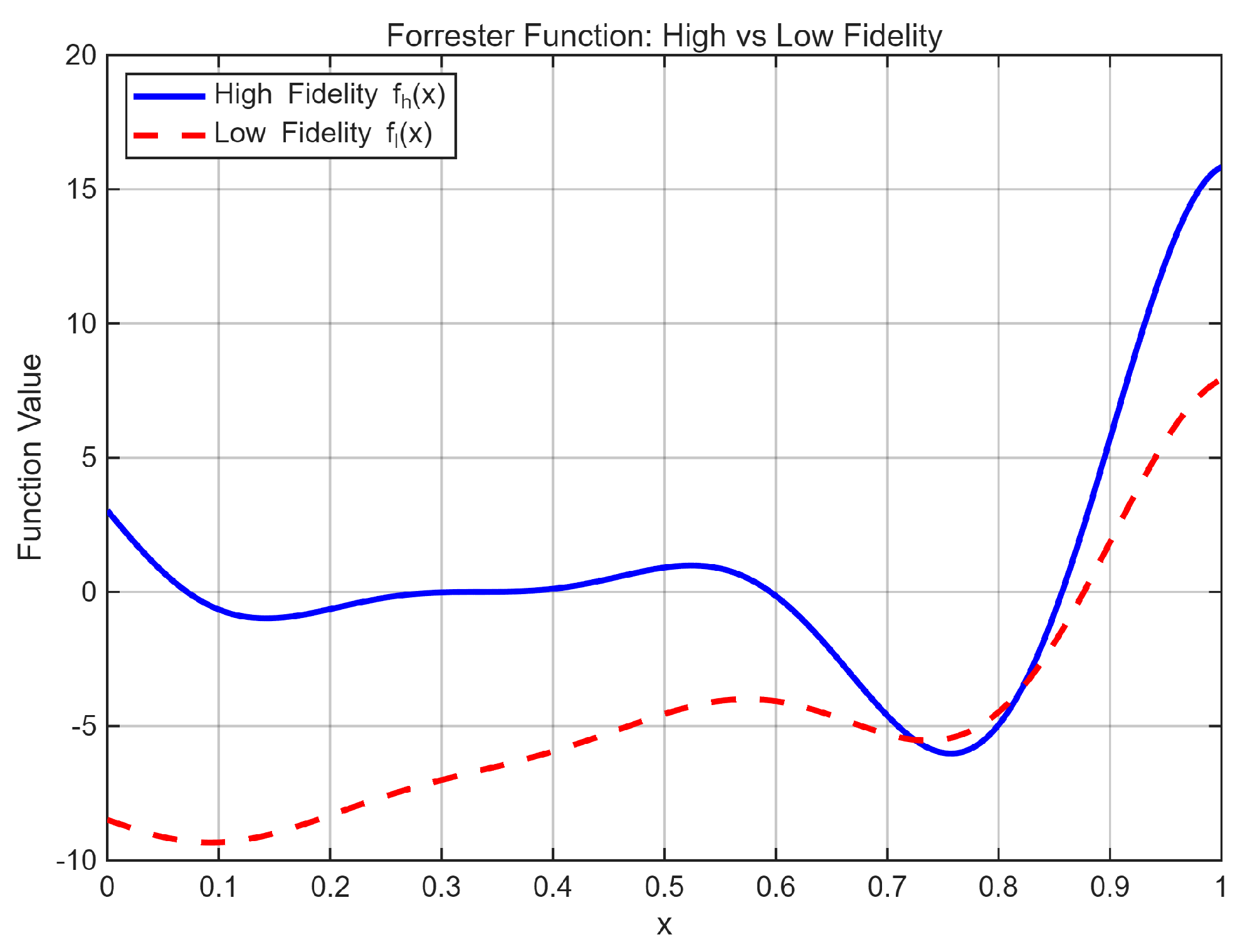
The Forrester function [36] is a classical one-dimensional multi-fidelity benchmark problem. Its high-fidelity and low-fidelity formulations are defined as follows (see the corresponding figure). The two models exhibit similar overall trends but differ significantly in local distribution characteristics, making the Forrester function widely used for validating multi-fidelity surrogate modeling methods.
f L ( x ) = ( 6 x 2 ) 2 sin ( 12 x 4 ) , f H ( x ) = f L ( x ) + 0.5 ( x 0.5 ) + ϵ ,
where x [ 0 , 1 ] and ϵ is a Gaussian noise term with zero mean.The low and high fidelity of the Forrester function is shown in Figure 2.
(2)
Airfoil Analysis Case
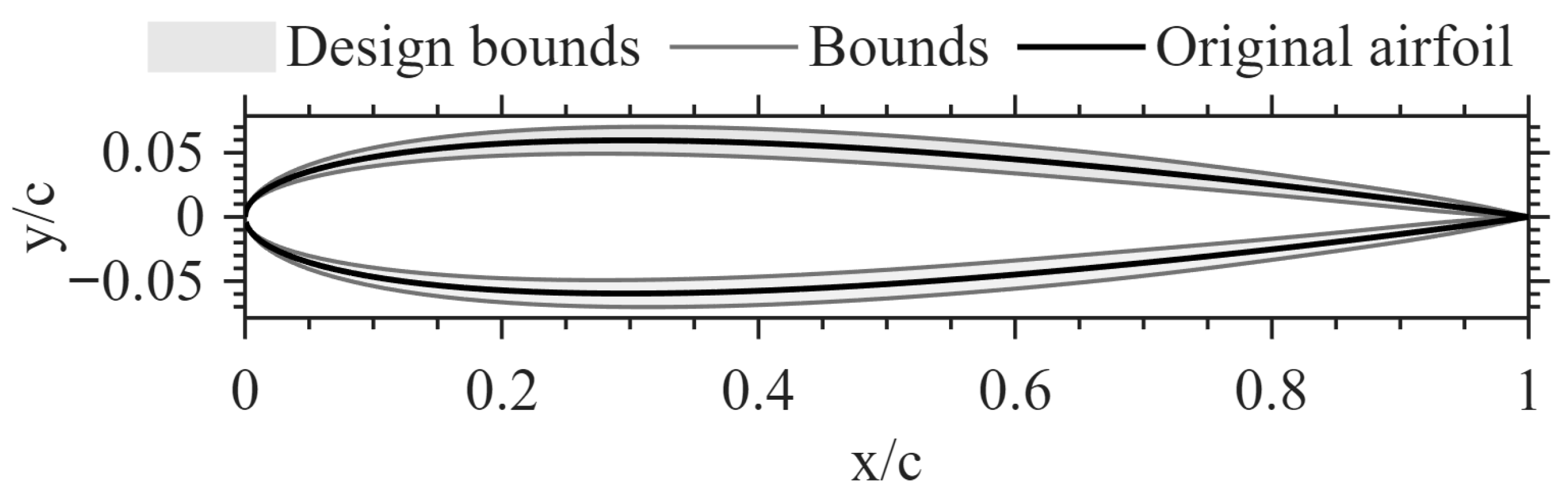
To further evaluate the prediction accuracy and engineering applicability of the proposed model, an airfoil aerodynamic analysis problem is selected as a representative example. Airfoil aerodynamic modeling is a typical task in aerospace engineering. In this study, the NACA 0012 airfoil is used as the baseline geometry, and shape variations are introduced using the Class–Shape Transformation (CST) perturbation method. Six CST control points are selected to modify the airfoil profile.
The lift coefficient ( C L ) and drag coefficient ( C D ) are chosen as model outputs. The baseline NACA 0012 geometry and the perturbation ranges of the CST [37] control points are shown in Figure 3. For aerodynamic analysis, a representative operating condition of angle of attack α = 5 deg and Reynolds number R e = 600,000 is adopted.
(3)
UAV with Strut-braced Wing Analysis Case
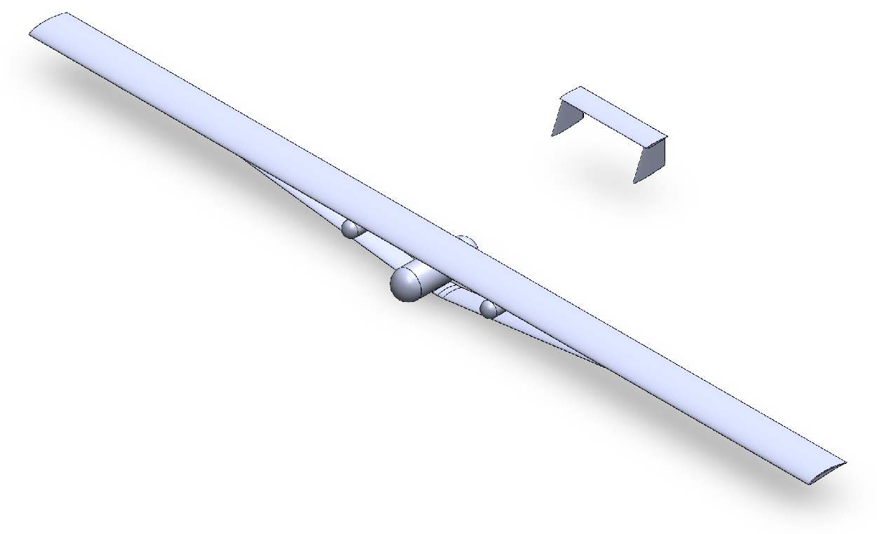
To further examine the proposed framework under a realistic three-dimensional aircraft configuration, a strut-braced wing UAV is selected as the engineering test case. The baseline aircraft configuration is adapted from the conceptual design study reported in [38], which developed an integrated scheme for a hybrid solar–hydrogen–lithium-battery UAV using a multi-attribute decision-making process. That study provides a consistent set of configuration parameters and performance-level information, forming a practical foundation for endurance-oriented UAV conceptual design and subsystem trade-off analysis.
Building upon this baseline configuration, the present work focuses on the aerodynamic evaluation and surrogate construction aspect and establishes a two-level aerodynamic analysis pipeline. Specifically, a low-fidelity (LF) aerodynamic model is constructed using a fast potential-flow-based method (e.g., vortex lattice/panel formulation) to enable large-scale sampling at a low computational cost, while a high-fidelity (HF) aerodynamic model is constructed using CFD based on RANS equations to provide reference-quality aerodynamic responses. Compared with the two-dimensional airfoil case, this three-dimensional strut-braced wing configuration introduces stronger geometric nonlinearity and interference effects (wing–strut junction, lift distribution changes, and drag penalties), making it a more stringent benchmark for evaluating transfer reliability and generalization in HF-scarce regimes. The aerodynamic outputs of interest are defined as the key performance indicators required by subsequent design optimization, including the lift coefficient ( C L ) and drag coefficient ( C D ).
The configuration of the UAV with strut-braced wing is shown in Figure 4.

5.1.2. Network Construction

All models were trained on the same workstation equipped with an Intel(R) Core i7-12700 CPU @ 2.1 GHz and an NVIDIA RTX 3060 Ti GPU with 24 GB RAM. Data were initialized using standard score normalization, and parameters were optimized via gradient descent using the Adam optimizer. To ensure fairness, all models were trained under identical hyperparameter settings.
A multilayer perceptron (MLP) was adopted as the surrogate network to capture knowledge in both the source and target domains. The typical form of the MLP is given by
f s ( x ) = W L σ W L 1 σ σ W 1 x + b 1 + + b L
where W i and b i represent the weight matrix and bias vector of the layer respectively, i = 1 , 2 , , L . To activate the function, the ReLU function is selected as the activation function. During the training process, mean square error was used as the loss function for the source domain network, and MSD loss was used as the loss function for the target domain network. The hyperparameters of the model were optimized to obtain the hyperparameters for the backbone network and low reliability mapping layer, achieving training for both the backbone network and low reliability mapping layer.
The structures of the source domain network and target domain network used are shown in Table 1.
To verify the effectiveness of the proposed active sampling strategy and transfer learning training approach, four algorithms were designed for comparison, combining different sampling and training strategies as summarized in Table 2. A conventional approach, known as the Hierarchical Kriging (HK) modeling method, is also adopted in this paper to demonstrate the superiority and advanced nature of the proposed method.
The definitions of the sampling and training strategies used in Table 2 are as follows:
1.
Random sampling: No active learning is applied. During initialization, 20 high-fidelity samples are randomly selected using the Latin Hypercube Sampling (LHS) method to retrain the model.
2.
Active sampling: New samples are selected by minimizing the proposed scoring criterion, as described in Section 3.1.
3.
GPR-assisted: A GPR surrogate model is built to approximate the scoring function and guide the selection of new samples, as detailed in Section 3.1.
4.
MSE loss: The network is trained using the Mean Squared Error (MSE) as the loss function.
5.
MSD loss: The proposed MSD composite loss is used for network training, as defined in Section 3.2.
To improve training efficiency and convergence stability, all source domain input data are normalized using min–max normalization as follows, scaling each feature into a comparable numerical range:
x i = x i min ( X ) max ( X ) min ( X ) , x i X
To enhance the robustness and generalization ability of the neural network, a dropout-based approximate Bayesian inference strategy is adopted in this study. Specifically, dropout layers are used both as a regularization mechanism during training and as the stochastic source for Monte Carlo (MC) inference during uncertainty estimation. In the source domain network, two fixed dropout layers are inserted after the first and second hidden layers, with dropout rates both set to 0.2. In the target domain fine-tuning stage, an additional dropout layer is dynamically introduced after the second hidden activation layer (i.e., between relu2 and fc3). Its dropout rate is adaptively updated during training according to a decay schedule, starting from 0.10 and gradually decreasing with the iteration stage, with a lower bound of 0.03.
For uncertainty estimation in active sample selection, MC inference is performed by keeping the dropout layers active at inference time. Each candidate sample is passed through the current surrogate network for T = 30 stochastic forward passes, and the corresponding predictive mean and predictive standard deviation are computed from these repeated evaluations. For multi-output regression problems, the standard deviation is averaged over all output dimensions to obtain a scalar uncertainty measure for each candidate point. This value is denoted as u i in the active learning criterion, then normalized to U i , and finally combined with the diversity term and the transfer consistency term to form the overall sample selection score. In contrast, during conventional deterministic prediction and final performance evaluation, standard inference is used without MC sampling.
During model transfer, a model-based transfer strategy is adopted: the parameters of the first four feature layers of the source network are frozen and transferred to the target domain network, while newly added target domain layers are randomly initialized. For performance evaluation, the coefficient of determination ( R 2 ) and the root mean squared error ( R M S E ) are used to assess model prediction accuracy, while training time is recorded as an indicator of computational efficiency. The performance indicators are calculated as follows:
R 2 = 1 ( y i y ^ i ) 2 ( y i y ¯ ) 2
R M S E = ( y i y ^ i ) 2 n
where y i is the actual value, y ^ i is the predicted value, and y ¯ is the mean of the actual values; n is the quantity of samples.

6. Numerical Studies and UAV Aerodynamic Analysis

To validate the effectiveness of the proposed active transfer learning-based multi-fidelity surrogate modeling approach, comprehensive numerical studies are conducted in this section. Generic benchmark problems, NACA 0012 airfoil aerodynamic analysis, and UAV with strut-braced wing aerodynamic analysis are employed to assess model accuracy, convergence behavior, and data efficiency under limited high-fidelity sampling conditions.
Through systematic comparisons with conventional surrogate modeling and multi-fidelity approaches, the experimental results demonstrate the advantages of the proposed method in terms of prediction accuracy, convergence speed, and robustness, highlighting its practical applicability to UAV aerodynamic analysis and design optimization tasks.

6.1. Case I: Forrester’s Function

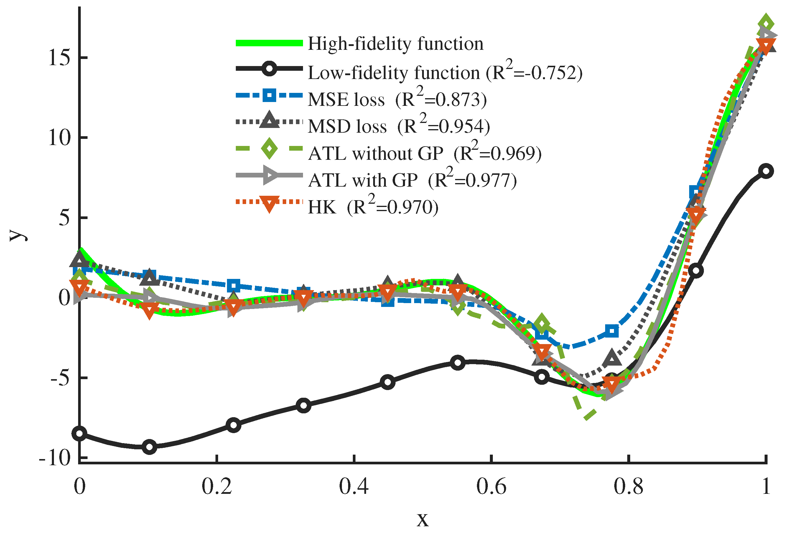
This section compares the surrogate model accuracy obtained in the Forrester function case. A total of 500 low-fidelity samples and 10 high-fidelity samples are used for model construction. During active learning, five iterations are conducted, and two samples per iteration are selected as new high-fidelity data points, forming the final surrogate model. The validation results are shown in Figure 5; the green solid line represents the actual high-fidelity model output, while the square, triangle, diamond, and arrow markers correspond to the predictions from Methods 1, 2, 3, and 4, respectively, as defined in Table 2.
From Figure 5, it can be observed that the proposed Gaussian process regression-assisted active transfer learning surrogate model (GPR-ATLSM) method achieves the best prediction accuracy compared with the other approaches. Both the MSD loss function and the active learning sampling criterion contribute effectively to improving the model’s predictive performance. It is worth noting that in Method 3 (ATL without GPR), when Gaussian process assistance is not used, the number of candidate points in the sampling pool is kept equal to that of the GPR-assisted case to ensure a comparable computational cost. A detailed sensitivity analysis of the GPR parameters and a runtime comparison are presented later in Section 6.6.
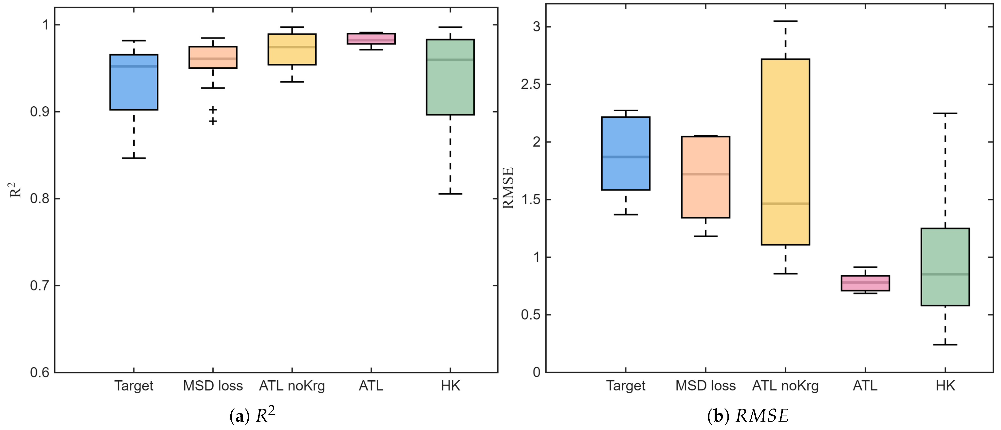
To eliminate experimental randomness, each algorithm was tested 20 times, and boxplots summarizing median, interquartile range, and outliers are shown in Figure 6. It can be observed that compared with other methods, GPR-ATLSM exhibits a higher median, indicating superior prediction accuracy, and a narrower interquartile range, indicating better robustness. The Hierarchical Kriging (HK) baseline exhibits an overall intermediate accuracy but noticeably weaker robustness compared with the proposed ATL-based models. Specifically, HK achieves a relatively high median R 2 and a moderate median R M S E , indicating that it can benefit from multi-fidelity information to improve prediction quality over the direct target-only baseline in many runs. However, the interquartile range (IQR) of HK is substantially wider, and the whiskers span a much larger range (especially in R M S E ), suggesting a pronounced sensitivity to training set realizations and occasional failure cases. This variability implies that the hierarchical correlation assumed by HK may become unstable under small-sample conditions or when the low-to-high fidelity discrepancy is non-stationary, leading to an inconsistent generalization performance. In contrast, the ATL framework (particularly with GPR assistance) yields a higher median performance with a tighter IQR, demonstrating superior stability and reliability.

6.2. Case II: Airfoil Aerodynamic Surrogate Modeling

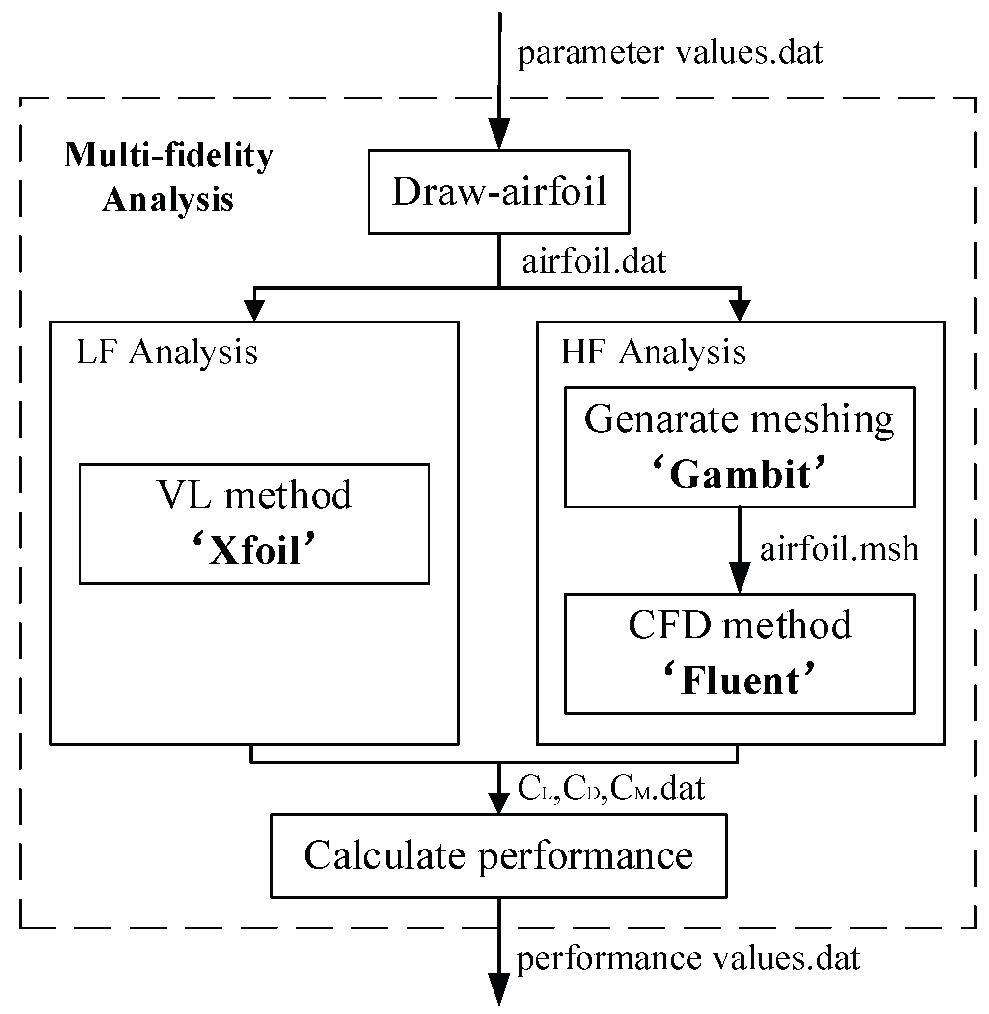
In this experiment, XFOIL is used for the rapid aerodynamic estimation of airfoil parameters, serving as the low-fidelity analysis model. A computational fluid dynamics (CFD) mesh suitable for airfoil analysis is then constructed, and numerical simulations are performed based on the RANS equations to serve as the high-fidelity analysis model.
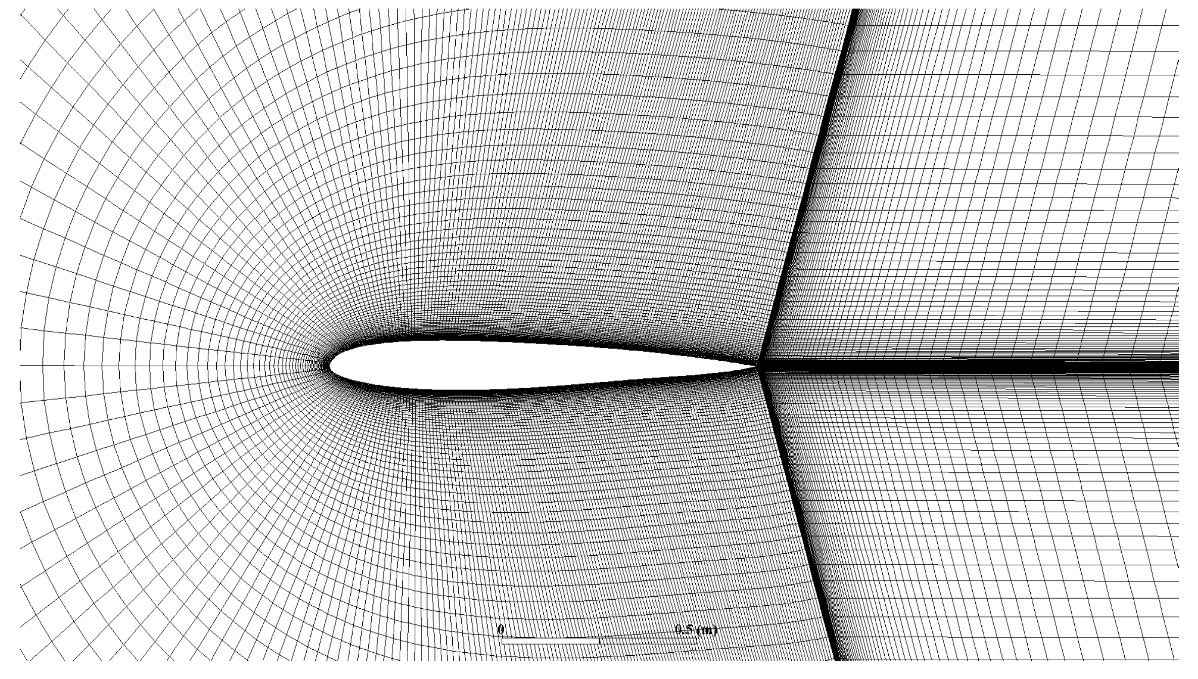
The workflow of the high- and low-fidelity aerodynamic analysis used in this study is illustrated in Figure 7, and the CFD airfoil mesh adopted for the high-fidelity simulations is also shown in Figure 8. Details of the analysis settings are provided in Appendix A.
Using the Latin Hypercube Sampling (LHS) method, 100 sample points were selected for low-fidelity analysis to form the source domain training set, while 15 sample points were used for high-fidelity analysis to construct the high-fidelity training set. The proposed GPR-ATLSM method was then applied to build the surrogate model, and its prediction accuracy was compared with that of other algorithms.
To eliminate experimental randomness, each algorithm was tested 20 times, and the results were statistically analyzed. The box plots of prediction accuracy for different algorithms are shown in Figure 9.
When comparing the airfoil surrogate models, the R 2 of the learning-based approaches are all close to unity, making R 2 alone less discriminative for ranking performance. Therefore, the mean relative error (MRE) is additionally reported as a complementary indicator to quantify relative deviations and to better reflect the practical prediction quality under repeated evaluations. As shown in the MRE, R 2 , and R M S E box plots in Figure 9, GPR-ATLSM provides a consistently favorable accuracy–robustness trade-off. Specifically, GPR-ATLSM achieves a mean R 2 of 0.9952 with a small dispersion (std 0.0007), while attaining the lowest mean R M S E (0.0162) and MRE (0.0667) among the compared methods. Relative to the target-only baseline, GPR-ATLSM reduces R M S E by 23.7 % and MRE by 43.3 % , and it yields a 55.0 % lower R M S E than the Hierarchical Kriging (HK) baseline, indicating improved predictive fidelity in both absolute and relative error metrics.
The ablation result further supports the contribution of the GPR-assisted component: removing it (ATL without Krg) leads to higher errors (mean R M S E 0.0197 and mean MRE 0.0815), suggesting that the proposed transfer mechanism improves generalization stability. Although the MRE distribution of GPR-ATLSM can occasionally exhibit outliers, this is consistent with the higher sensitivity of relative error measures. The R 2 and R M S E box plots show a tighter interquartile range, implying reduced variability across evaluation conditions. Overall, these results indicate that GPR-ATLSM is a reliable surrogate modeling strategy for airfoil aerodynamic analysis, and it is well suited for downstream tasks such as aerodynamic optimization where both accuracy and robustness are required.

6.3. Case III: UAV with Strut-Braced Wing Analysis Surrogate Model

The experimental settings follow those adopted in the NACA 0012 airfoil case to ensure consistency across case studies. In this SBW (strut-braced wing) UAV aerodynamic problem, a set of geometric sizing parameters is selected as the design variables, while the lift and drag coefficients, denoted by C L and C D , are used as model outputs. The considered design variables and their bounds are summarized in Table 3.
To construct the surrogate models, Latin Hypercube Sampling (LHS) is employed throughout the experiment. During initialization, 100 samples are evaluated using the low-fidelity (LF) aerodynamic model and five samples are evaluated using the high-fidelity (HF) model. The learning process then proceeds for five iterations. At each iteration, the proposed active sampling strategy selects two additional samples for model refinement, until the final surrogate model is obtained.
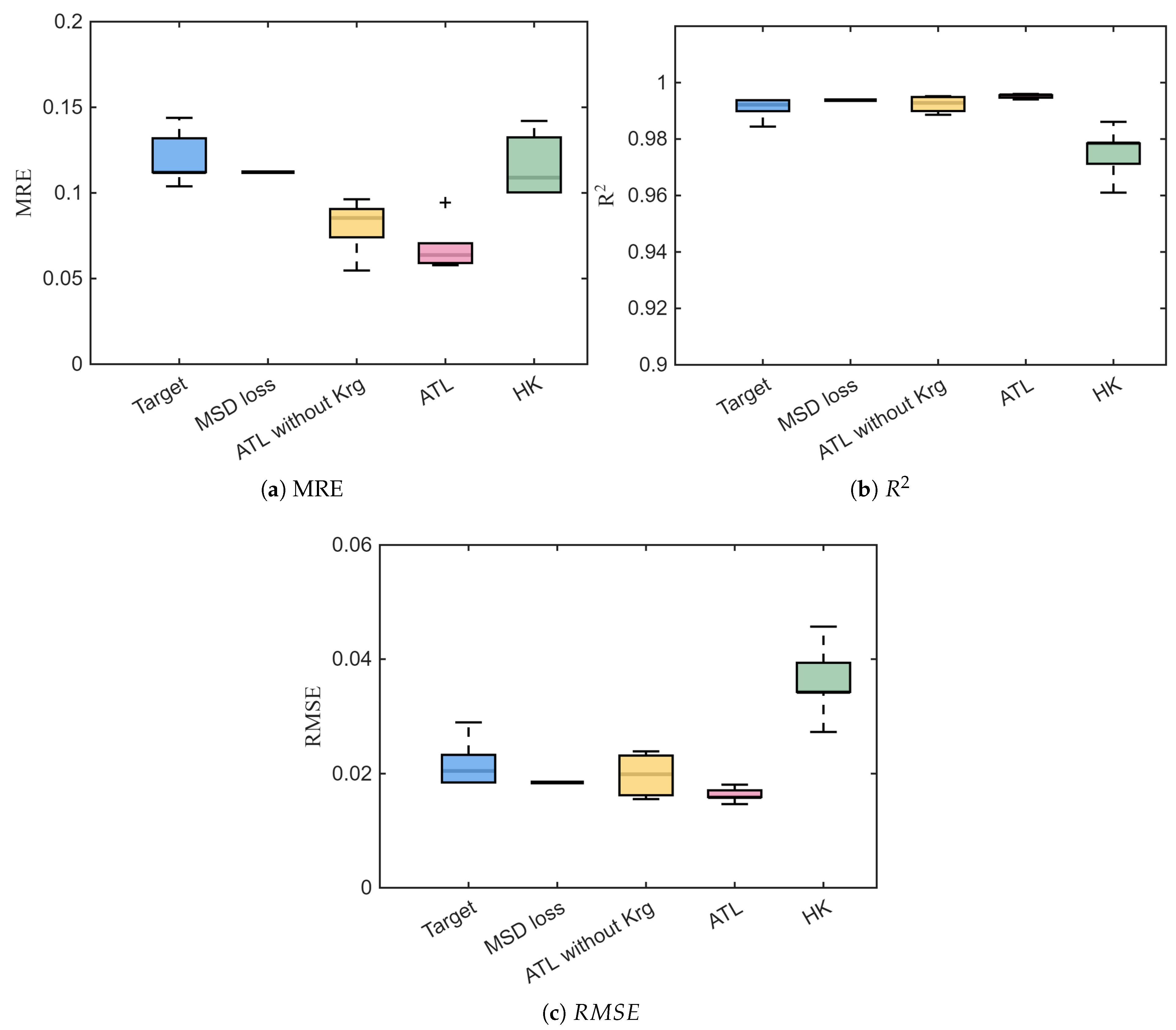
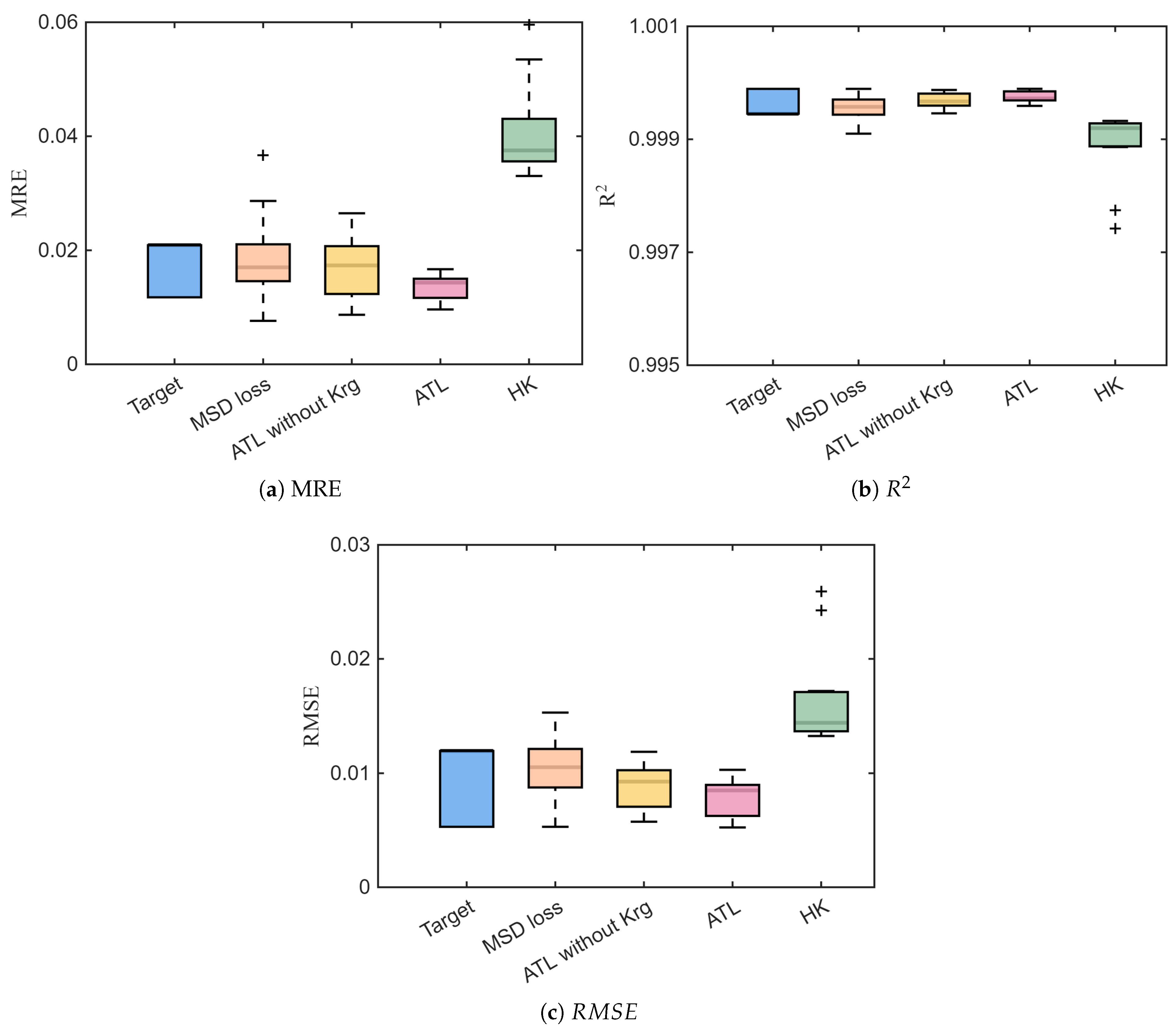
Model performance is assessed using three complementary metrics: mean relative error (MRE), root mean square error ( R M S E ), and the coefficient of determination ( R 2 ). To mitigate randomness induced by sampling and training variability, each competing method is independently repeated 15 times, and the resulting statistics are reported using boxplots (Figure 10).
Figure 10 compares the prediction error distributions of different surrogate construction strategies on the SBW UAV aerodynamic problem in terms of MRE, R M S E , and R 2 . The compared approaches include the target-only baseline (Target), a transfer method based on MSD loss, an ablated variant without Kriging correction (ATL without Krg), the complete active transfer learning approach (ATL), and the conventional Hierarchical Kriging (HK) model.
In terms of MRE and R M S E , the proposed ATL achieves the lowest median errors and exhibits a notably smaller interquartile range than the other methods, indicating not only superior average predictive accuracy but also improved robustness across repeated trials. In contrast, ATL without Krg shows a clear degradation in error levels, suggesting that relying solely on transfer learning without explicitly modeling the high-fidelity residuals is insufficient to capture the strong nonlinearity and coupling effects inherent in SBW aerodynamic responses.
The MSD-loss-based transfer method improves upon the Target baseline to some extent; however, its error distributions remain relatively dispersed with visible outliers, implying limited adaptability to structural discrepancies between the source and target domains. The HK model yields the weakest performance across all three metrics; in particular, its MRE and R M S E are substantially higher than those of the active transfer learning approaches, highlighting the limitations of purely hierarchical co-kriging under scarce HF data and pronounced configuration differences.
For R 2 , ATL maintains values close to unity with the smallest dispersion among all methods, further confirming a favorable balance between global trend learning and local high-fidelity correction. By comparison, HK not only presents a lower average R 2 but also produces pronounced abnormal points, indicating an inadequate generalization capability for this high-dimensional, strongly coupled SBW aerodynamic design task.
Overall, these results demonstrate that the proposed active transfer learning framework with Kriging-based correction can significantly enhance both predictive accuracy and stability, making it particularly suitable for SBW UAV aerodynamic modeling problems characterized by high dimensionality and strong nonlinearity.

6.4. Ablation Experiment Design

To further investigate how different components of the proposed method affect network performance, we conduct an ablation analysis using Test Case I. Key factors are selected and compared to assess their impact on the model.

The Impact of Loss Function Weights

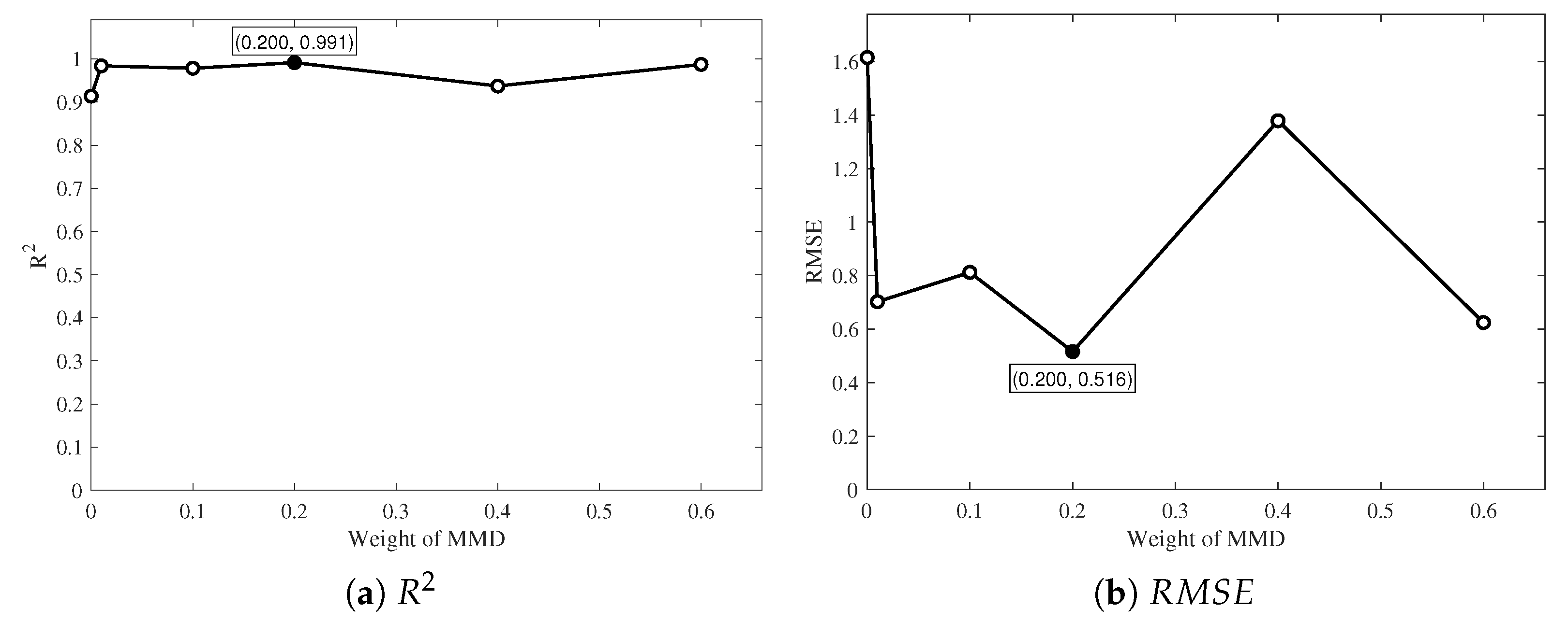
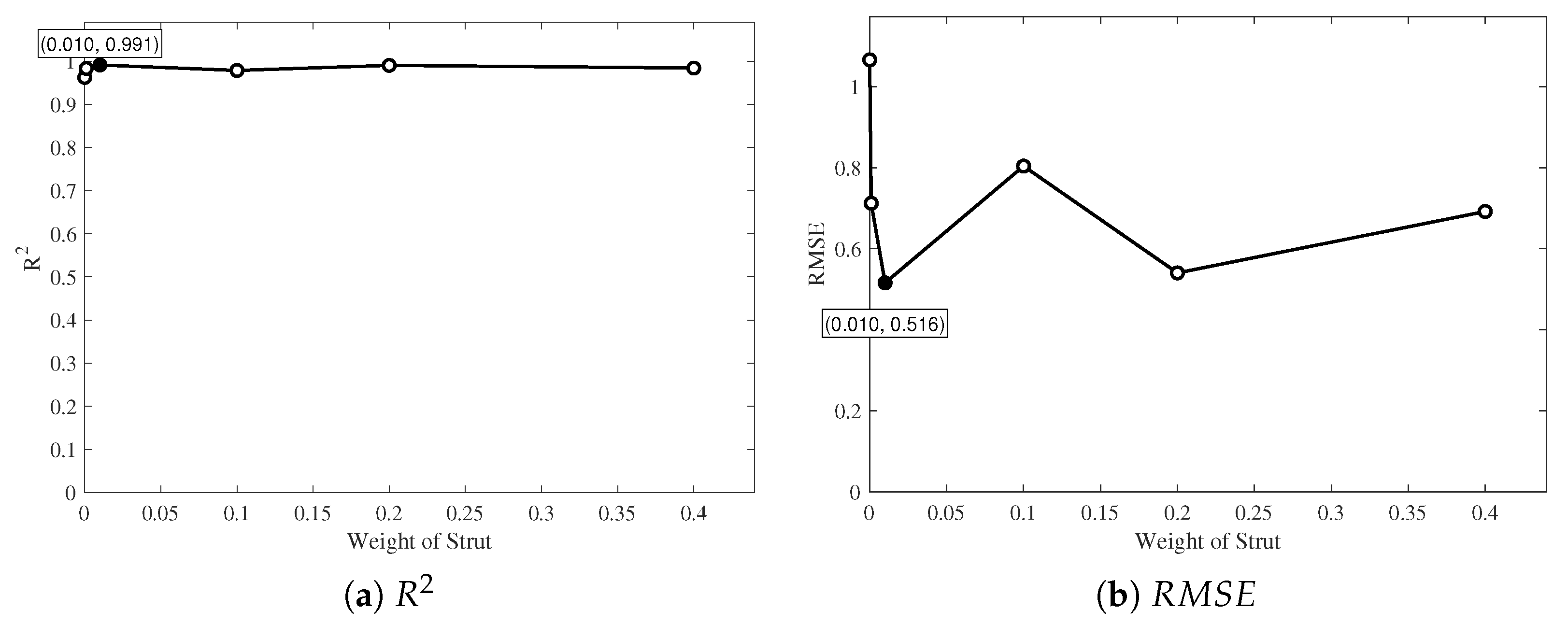
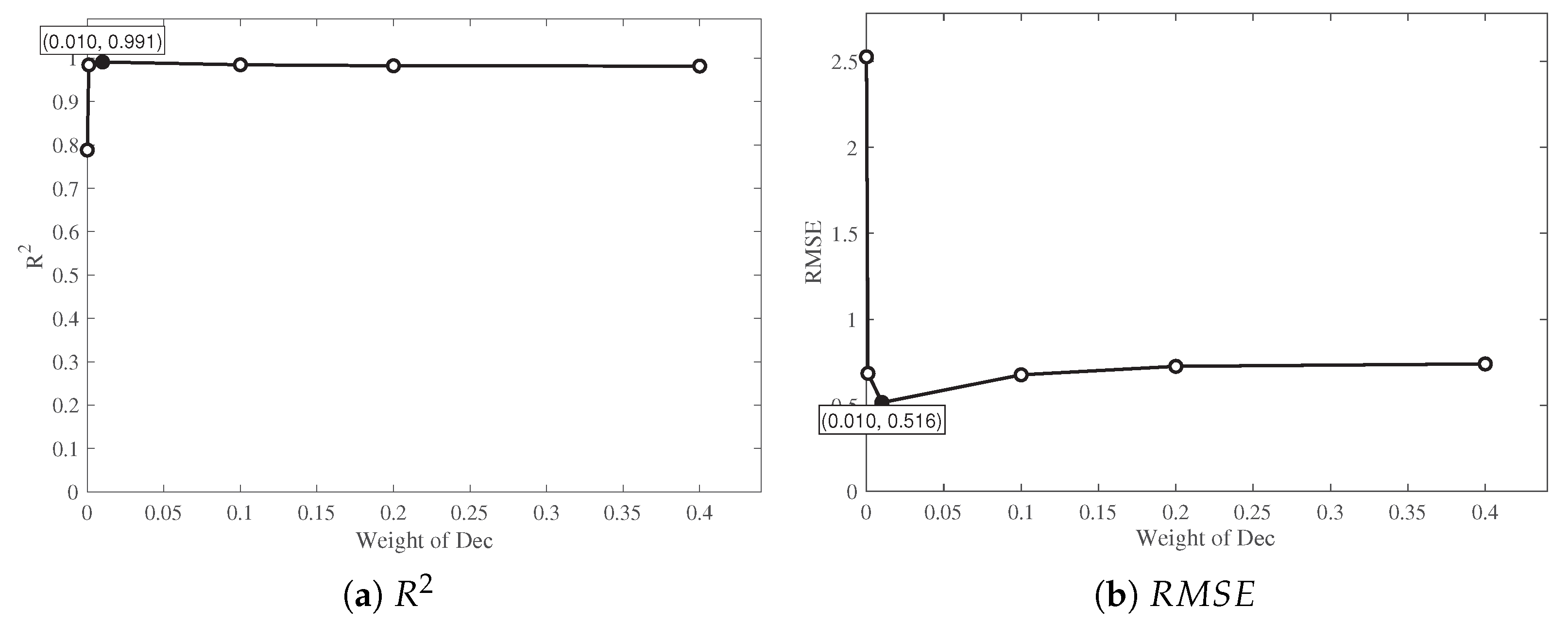
In this subsection, we design ablation experiments based on the loss function in Equation (20) and analyze the R 2 and R M S E performance. The computed results are presented in Figure 11, Figure 12 and Figure 13.
It can be seen in Figure 11 that when the weight of MMD is 0 (i.e., without MMD loss), the R 2 and R M S E performance indicators of the model are significantly inferior to those with MMD loss. However, when MMD loss is introduced, even with a smaller weight, the prediction accuracy of the model can be significantly improved. When the MMD loss weight is 0.2, the performance of the model is optimal.
When introducing structural loss, the performance of the model also improves to a certain extent, especially when focusing on the R M S E performance indicator; the mean square error of the model is reduced by 50 % compared with the case where the structural loss weight is 0. When the structural loss weight is 0.01, the performance of the model is optimal.
From Figure 13, it can be seen that the performance of the model is significantly improved when feature decoupling loss is introduced. The main reason is that this loss focuses on the cross-domain generalization ability from the source domain to the target domain, enhancing the effectiveness of transfer learning. When the feature decoupling loss weight is 0.01, the model performance is optimal.

6.5. The Impact of Active Learning Function Weights

In the active learning stage, a new criterion for adding points to active learning was proposed. This section designs ablation experiments and analyzes R 2 and R M S E . The calculation results are shown in Figure 14.
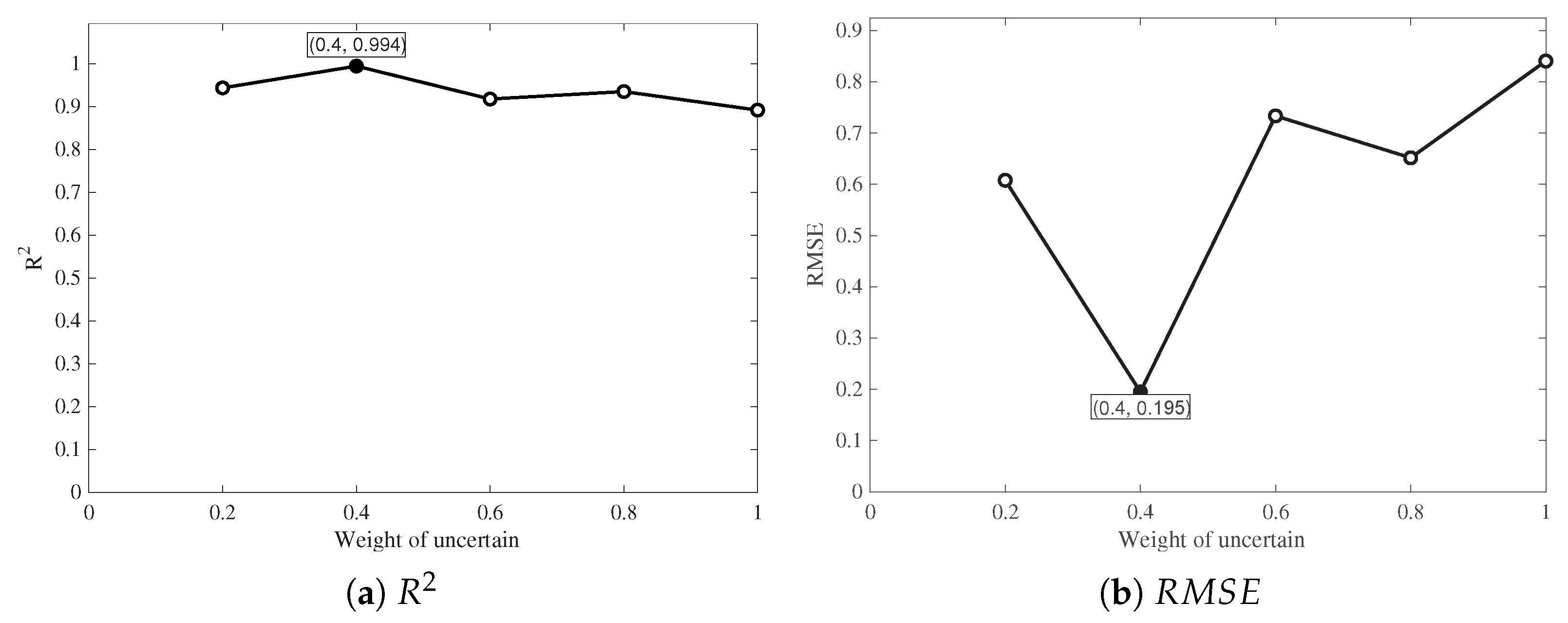
It can be observed from Figure 14 that when the uncertainty weight is small, the robustness of the model is low. Appropriately increasing the uncertainty weight improves the model’s robustness; however, when the uncertainty weight is excessively large, a phenomenon occurs during the iteration process: when updating training points, the training points cluster in areas with high uncertainty, ignoring the overall performance, which further leads to a decline in model accuracy.
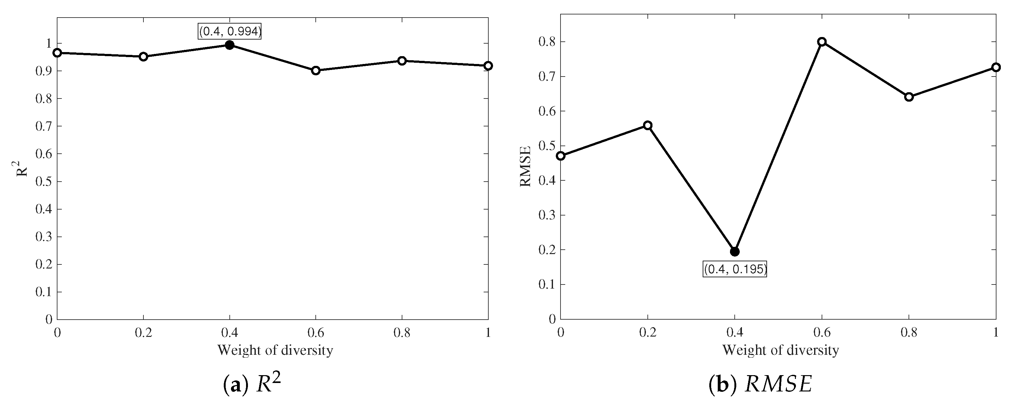
When diversity is introduced, it can be observed from Figure 15 that the performance of the model increases. However, when the diversity weight is excessively large, the model also exhibits a problem of performance degradation. This is mainly because an excessive focus on diversity prevents more sample point updates in areas with poor accuracy.
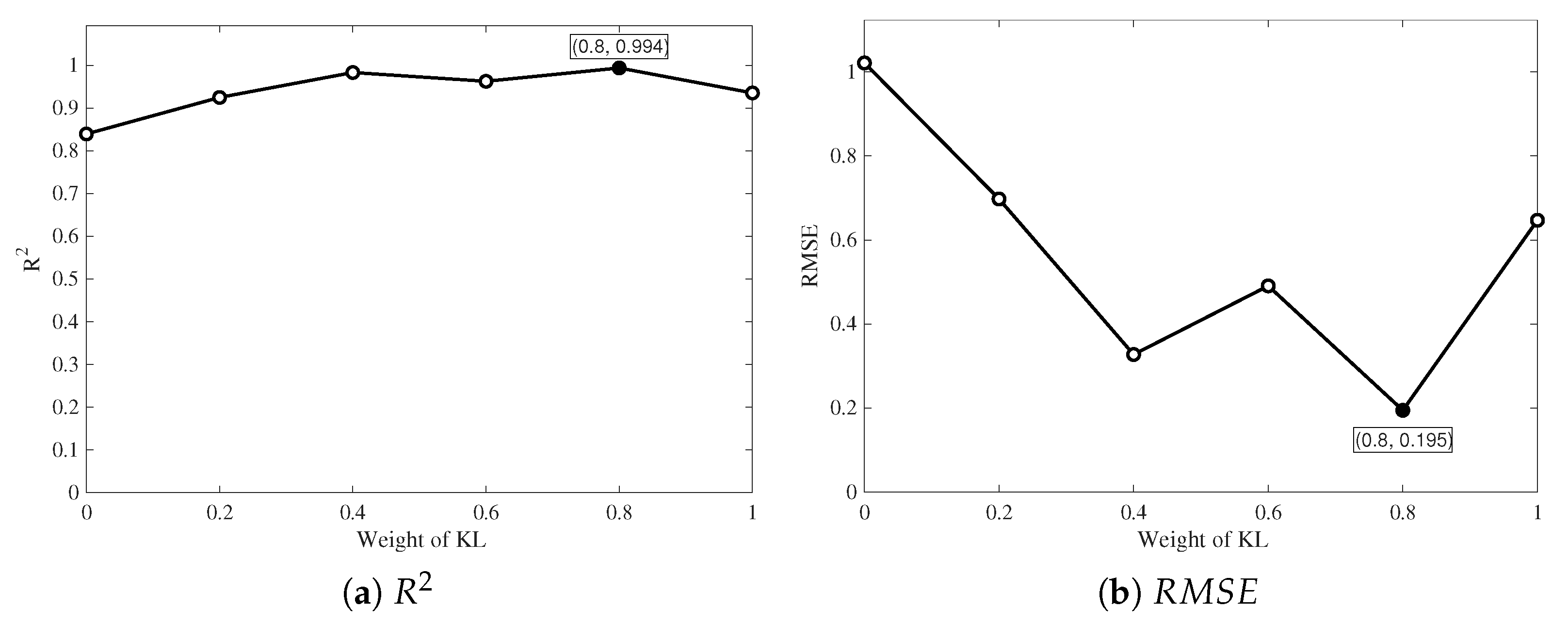
When focusing on the KL divergence weight, it can be observed from Figure 16 that the overall performance improves as the KL weight increases, reflected by higher R 2 and generally lower R M S E . This is mainly because KL divergence enables better exploration of the similarity relationships between the source domain and the target domain, thereby guiding the active learning model to select new sample points. The model achieves an optimal performance when the KL divergence weight is set to 0.8.

6.6. The Impact of Gaussian Process Regression Assistance

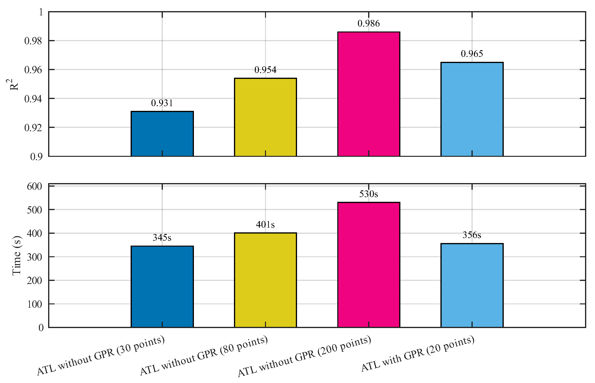
This subsection primarily explores the impact of the active learning method assisted by GPR on model performance. GPR can effectively reduce the computational load during the active sample addition process and improve computational efficiency. The model establishment accuracy under different numbers of candidate points was analyzed. To calculate uncertainty and KL divergence, the number of uncertainty predictions was set to 10,000. The average value was obtained after 10 calculations, and the performance indicators under various working conditions are presented in Table 4 and Figure 17.
As can be observed from Table 4 and Figure 17, when the Gaussian process is employed to assist active transfer learning, the R 2 performance is higher than that of active transfer learning without Gaussian process assistance when only small candidate pools are affordable. This is mainly because Gaussian process-assisted active learning enables the selection and calculation of optimal candidate points on a global scale, rather than being limited to a small number of points in the candidate pool. With GPR assistance, ATL achieves better accuracy than ATL without GPR when only small candidate pools are affordable (e.g., 20 vs. 30/80 points), while maintaining a lower computational burden than using a much larger candidate pool without GPR. Although ATL without GPR can reach a higher R 2 when the pool size is expanded to 200, its computation time rises to about 1.5 times that of the GPR-assisted setting. The above data verifies the effectiveness of the proposed Gaussian process-assisted active learning method in the process of active sample addition.


7. Conclusions and Future Work

This paper presents an ATL-based multi-fidelity surrogate modeling method that combines GPR-assisted active sampling and a multi-term transfer. Through numerical and aerodynamic analysis benchmarks, the proposed approach demonstrates superior modeling efficiency and accuracy under HF data conditions. The main conclusions are summarized as follows:
1.
A multi-fidelity surrogate modeling method based on active transfer learning is proposed, in which low-fidelity and high-fidelity analysis data are treated as the source domain and target domain datasets, respectively. This approach enables an efficient modeling process under small-sample conditions.
2.
The proposed transfer learning loss function effectively captures the implicit relationships between the source and target domains, thereby improving training efficiency. Moreover, the model update strategy maintains feature consistency and accelerates model convergence during the transfer process, further enhancing the stability and accuracy of the surrogate model.
3.
The engineering applicability of the proposed method is validated on airfoil and UAV with strut-braced wing aerodynamic surrogate modeling cases. Under a highly HF-limited setting (only 15 HF samples), the proposed approach achieves an MRE below 5%, demonstrating strong sample efficiency and practical accuracy for aerodynamic analysis and optimization.
4.
Ablation experiments were designed to evaluate the contributions of each proposed performance metric during both the transfer learning and active learning stages. Comparative results indicate that the inclusion of these metrics consistently improves performance, yielding higher R 2 values and lower R M S E compared with models that omit them.
5.
The integration of GPR into the active learning stage enables the efficient computation of sample performance metrics, using the EI as the selection criterion. The experimental results demonstrate that this GPR-assisted sampling strategy enhances model accuracy under the same computational cost.
Future work will focus on scaling the ATL framework to UAV-level applications, where aerodynamics and structural responses are tightly coupled and the design space is high-dimensional. We plan to develop multi-fidelity surrogates for integrated aerodynamic and structural evaluations and to embed physics-informed constraints, thereby supporting efficient multidisciplinary design optimization for full-airframe UAV configurations.

Author Contributions

D.Y.: Conceptualization, Methodology, Formal analysis, Visualization, Writing—Original Draft, Writing—Review and Editing. L.L.: Validation, Writing—Review and Editing, Supervision. B.Y.: Methodology (Optimization Guidance), Validation, Writing—Review and Editing. All authors have read and agreed to the published version of the manuscript.
Funding

The authors did not receive support from any organization for the submitted work.

Data Availability Statement

The code and data supporting the findings of this study are available from the corresponding author upon reasonable request. Specifically, the following materials can be provided: the implementation of the proposed active transfer learning framework, including network architecture definition, training procedure, and active learning strategy; the aerodynamic analysis codes used for airfoil evaluation, including both low-fidelity and high-fidelity models; the UAV aerodynamic analysis scripts used for generating simulation data in this study; the processed datasets used for model training and testing, as well as instructions for reproducing the experimental workflow. Due to computational environment dependencies and project organization constraints, the code is not publicly released at this stage but can be shared upon request for research purposes.

Acknowledgments

The authors would like to thank the anonymous reviewers for their valuable comments and suggestions, which helped to improve the quality of this manuscript.

Conflicts of Interest

The authors declare that they have no competing interests to declare that are relevant to the content of this article.

Appendix A. Multi-Fidelity Analysis Setting for UAV Cases

Reproducibility Details for the Airfoil CFD Case

To strengthen the reproducibility of the airfoil CFD case, this appendix summarizes the complete solver setup, boundary conditions, mesh parameters (including near-wall y + targets), convergence criteria, and key neural network (NN) training hyperparameters used in this study.
(1)
CFD software and workflow
The airfoil simulations were conducted using ANSYS Fluent (v17.0) with mesh generation performed in GAMBIT (v2.3.16). The entire CFD workflow was automated via journal files for repeatable meshing and solving (e.g., airfoil_Gambit.jou and airfoil_Fluent.jou), enabling batch evaluation of CST-perturbed airfoil geometries.
(2)
Governing equations, turbulence model, and material properties
A steady RANS formulation was adopted for the airfoil analyses. Since the operating Reynolds number is on the order of 10 5 10 6 , the flow was treated as subsonic and (effectively) incompressible in a pressure-based steady solver. Air properties were set to standard sea-level values, with density and viscosity specified consistently (e.g., ρ = 1.225   kg / m 3 and μ = 1.789 × 10 5   Pa · s ). The turbulence closure employed the SST k ω model to balance near-wall accuracy and separation prediction, with a near-wall resolution target of y + 1 .
(3)
Computational domain and boundary conditions
A 2D C-type outer domain was adopted to minimize far-field interference. The far-field boundary was placed sufficiently far from the airfoil (typical extents: upstream 10 c , downstream 15 c , and normal directions 15 c ) to ensure negligible boundary impact on the near-field solution. Boundary conditions were specified as follows:
  • Inlet (freestream): velocity inlet with prescribed V and angle of attack α ;
  • Outlet: pressure outlet (gauge pressure = 0 );
  • Upper/lower far-field boundaries: symmetry (or equivalent freestream/symmetry treatment);
  • Airfoil surface: no-slip wall.
Turbulence quantities at the inlet were specified using a standard turbulence viscosity ratio (e.g., μ t / μ = 10 ) when needed.
(4)
Mesh parameters and y + control
A structured quadrilateral mesh was generated around the airfoil and mapped to the domain blocks. The mesh seeding strategy was as follows:
  • Airfoil surface (upper/lower): 150 intervals (uniform ratio);
  • Normal direction (near-airfoil block edges): 100 intervals with geometric stretching toward the wall;
  • Outer arc boundary: 300 intervals with double-sided stretching (denser near junctions);
  • Remaining outer edges: 100 intervals with mild stretching.
To satisfy the near-wall modeling requirement of SST k ω , an inflation layer was applied near solid walls with eight prism layers and a first-layer height of 0.01 mm, targeting y + 1 . Mesh quality was verified using standard checks (e.g., positive cell volumes and reasonable skewness). A mesh independence check was performed to confirm that increasing grid size beyond the selected mesh does not significantly change C L and C D .
(5)
Numerical schemes and convergence criteria
The pressure–velocity coupling used SIMPLE (s pressure-based steady solver). Spatial discretization employed second-order schemes (e.g., second-order upwind for convection terms) to improve accuracy. Convergence was declared when
1.
Residual criterion: all governing equation residuals dropped below 10 3 ;
2.
Force stability: monitored aerodynamic coefficients ( C L , C D ) reached a statistically steady plateau (change below 10 4 over at least 100 iterations).
In practice, a maximum of 250 iterations was allowed per case, and most cases converged within ∼200 iterations. Aerodynamic coefficients were obtained via Fluent’s built-in force integration on the airfoil wall boundaries.
Table A1. Summary of CFD solver setup for the airfoil case (for reproducibility).
ItemSetting
SoftwareANSYS Fluent v17.0; GAMBIT v2.3.16; automated journal-based workflow
Flow modelSteady RANS; pressure-based steady solver; subsonic/incompressible assumption
Turbulence modelSST k ω ; near-wall target y + 1
Fluid propertiesSea-level air (e.g., ρ = 1.225   kg / m 3 , μ = 1.789 × 10 5   Pa · s )
Domain2D C-type far-field; typical extents ( 10 c , + 15 c ) streamwise and ± 15 c normal
BCsVelocity inlet ( V , α ); pressure outlet; symmetry far-field; no-slip wall on airfoil
MeshStructured quads; 150 intervals on airfoil; 100 normal; 300 far-field arc; stretching toward wall
Near-wall mesh8 inflation layers; first-layer height 0.01 mm; y + 1
SchemesSIMPLE; second-order spatial discretization
ConvergenceResiduals < 10 3 and C L / C D stable (< 10 4 change over 100 iterations)

Appendix B. Multi-Fidelity Analysis Setting for UAV Cases

Building upon the strut-braced wing configuration, the present study develops both high-fidelity and low-fidelity aerodynamic analysis models to perform hierarchical aerodynamic evaluation and comparative assessment.

Appendix B.1. High-Fidelity Aerodynamic Analysis Method

Considering that the cruise Mach number of the investigated low-speed UAV is well below 0.3, the flow is assumed to be steady, incompressible, and subsonic. The incompressible RANS equations are solved using ANSYS Fluent; all of the workflow are constructed on the Workbench platform.
(1)
Geometry Modeling and Computational Domain
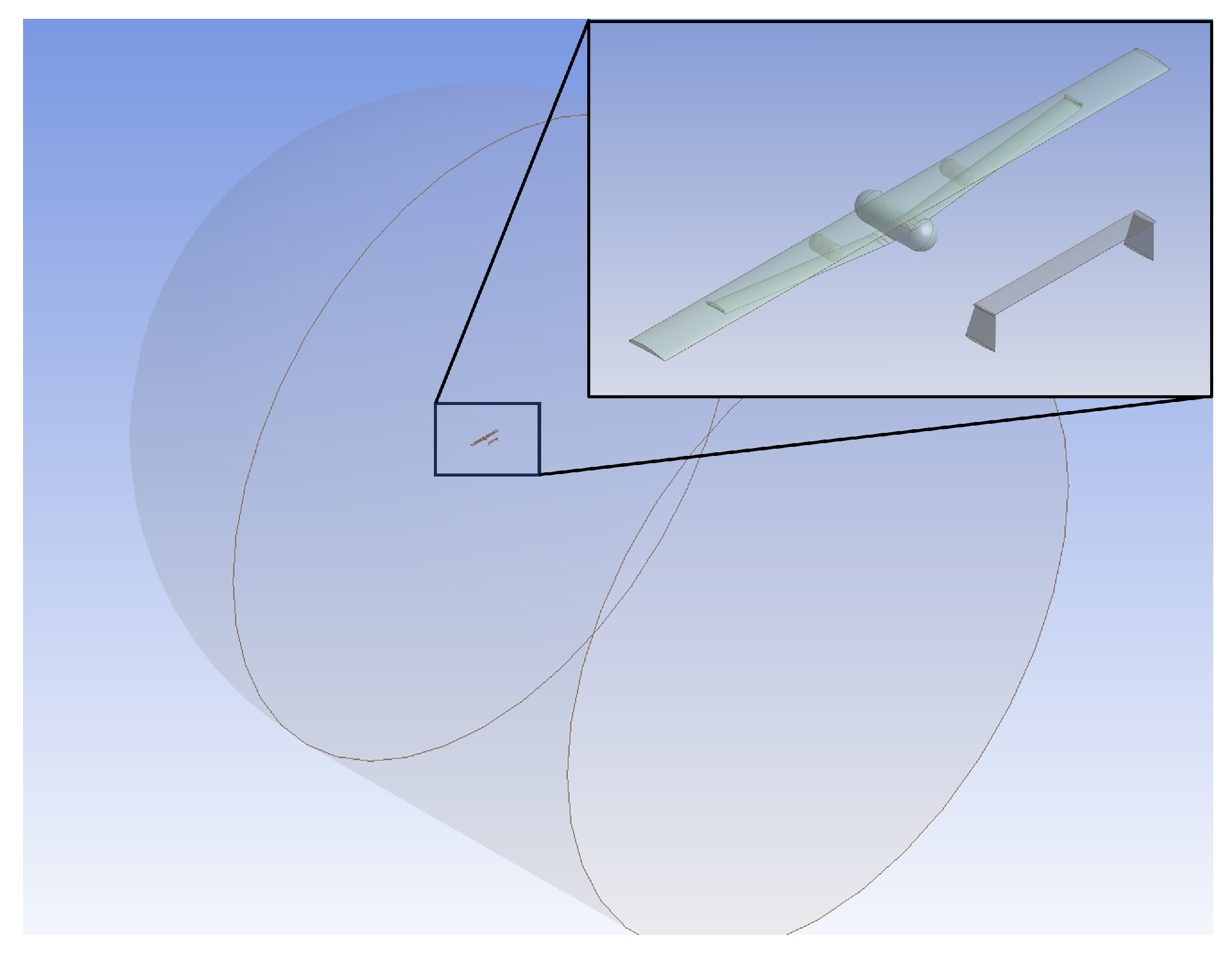
A full external configuration model was established, including the main wing, strut wing, horizontal and vertical tails, fuselage, and external hydrogen tanks. To improve numerical stability and convergence, rotating components such as propellers were neglected, allowing the analysis to focus on the intrinsic aerodynamic characteristics of the airframe.The computational domain was defined as a far-field external flow region, ensuring that boundary effects do not influence the flow solution around the UAV. The computational domain used in this case study is shown in Figure A1.
Figure A1. The computational domain of UAV.
Drones 10 00290 g0a1
(2)
Mesh Generation and Grid Independence Study
An unstructured tetrahedral mesh was employed for spatial discretization. To accurately resolve near-wall flow features, eight layers of prism boundary layer elements were generated adjacent to solid surfaces, with a first-layer height of 0.01 mm. Given the adoption of the SST k ω turbulence model, the near-wall resolution was controlled to maintain y + 1 .
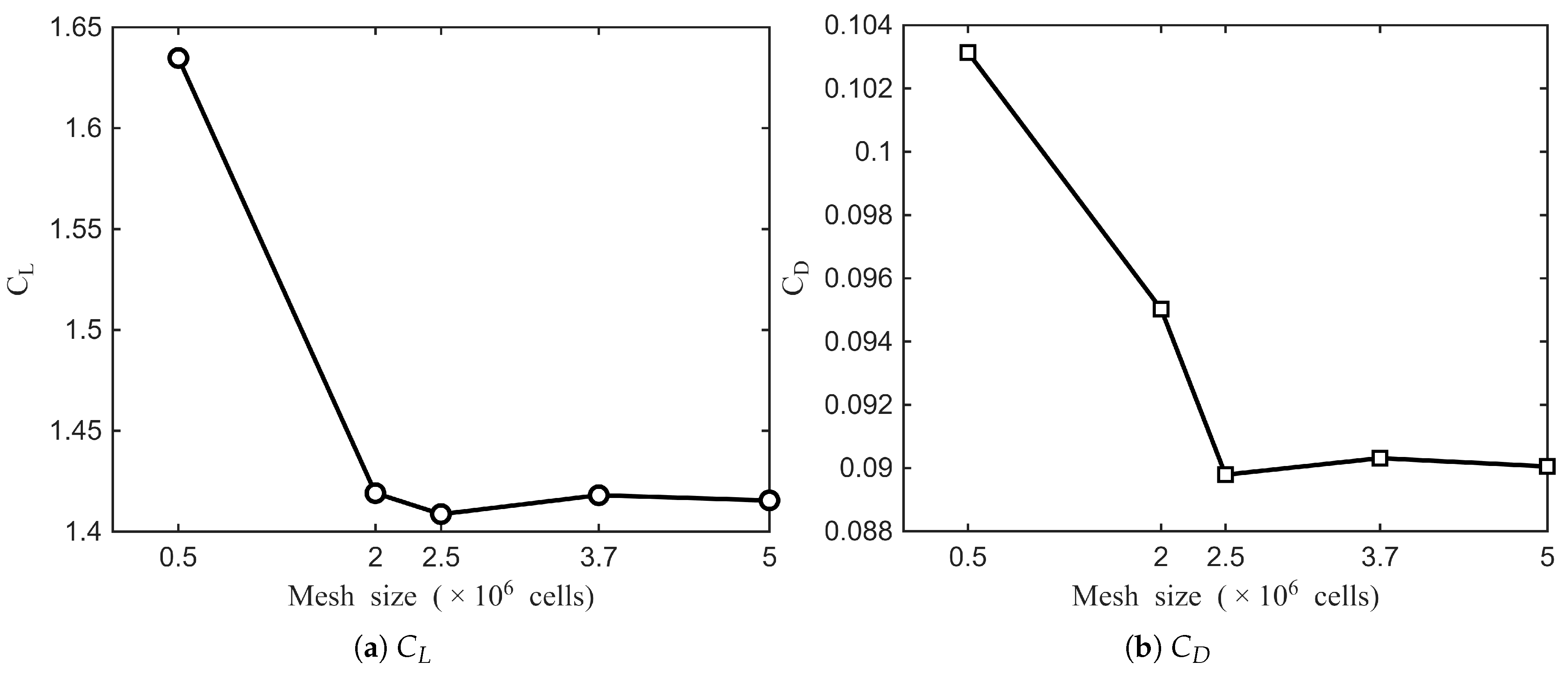
A grid independence study was performed at α = 5 , V = 15   m / s . As shown in Figure A2, the variations in the lift coefficient C L and drag coefficient C D with respect to mesh density were evaluated.
Figure A2. Variations in C L and C D with respect to mesh density.
Drones 10 00290 g0a2
It was observed that C L converges satisfactorily at approximately 2 million cells; C D exhibits higher sensitivity to mesh resolution; and both coefficients become nearly invariant when the mesh exceeds 2.5 million cells. Accordingly, a mesh size of approximately 2.5 million cells was selected for subsequent high-fidelity simulations.
(3)
Boundary Conditions and Solver Settings
The boundary conditions were specified as follows:
  • Velocity inlet with prescribed freestream velocity V = 15  m/s and corresponding angle of attack;
  • Pressure outlet;
  • Far-field symmetry boundaries for lateral and vertical outer surfaces;
  • No-slip wall condition on all solid surfaces.
Air properties were defined under standard sea-level conditions as follows:
ρ = 1.225   kg / m 3 , μ = 1.789 × 10 5   Pa · s
A pressure-based steady-state solver was adopted. Given a Reynolds number range of 10 5 10 6 , the flow remains subsonic and incompressible.
The SST k ω turbulence model was selected for its robustness in predicting both near-wall shear flows and boundary layer separation. Pressure–velocity coupling was handled using the SIMPLE algorithm. Second-order spatial discretization schemes were employed, and the convergence criterion for residuals was set to 10 3 .
(4)
Post-Processing
The lift coefficient C L and drag coefficient C D were obtained via surface force integration within Fluent.

Appendix B.2. Low-Fidelity Aerodynamic Analysis Method

NASA [39] indicates that a decomposition-based methodology is suitable for low-fidelity drag estimation of strut-/truss-braced wing configurations. Following this guidance, this study develops a low-fidelity drag correction strategy on top of the VLM/AVL-predicted induced drag to compensate for the limited capability of VLM in predicting viscous zero-lift drag and interference drag. The UAV is decomposed into major lifting components (main wing, strut wing, horizontal tail, and vertical tail), while additional drag contributions from the fuselage and external hydrogen tanks are incorporated as additive terms to obtain an engineering-level total drag estimate.
(1)
Total Drag Decomposition
Since VLM provides reliable lift distribution and induced drag, the total drag coefficient is decomposed as
C D = C D i + C D 0 .
where C D is the total drag coefficient; C D i is the induced drag coefficient (obtained from AVL); and C D 0 is the zero-lift drag coefficient requiring viscous/interference correction.
Accordingly, the corrected total drag coefficient is defined as
C D corr = C D i + C D 0 corr .
where C D 0 corr denotes the corrected zero-lift drag coefficient. The corrected zero-lift drag is decomposed into
C D 0 corr = C D , f + C D , p + C D , i n t + C D , b a s e .
where C D , f is skin friction drag, C D , p is pressure/form drag, C D , i n t is interference drag, and C D , b a s e is base drag.
(2)
Engineering Estimation of Friction and Form Drag
Following the drag build-up concept, friction/form drag can be categorized into skin friction drag, pressure (form) drag, and lift-dependent drag. The lift-dependent term is often negligible for the low-speed cruise and small angles of attack of interest and is ignored in this work. The combined friction and form drag of a given component is estimated using
C D , f p = C f · F F · S w e t S r e f .
where C D , f p is the component drag coefficient due to friction and form effects; C f is the equivalent flat-plate skin friction coefficient; F F is the form factor; S w e t is the wetted area of the component; and S r e f is the reference area (typically the wing reference area).
(3)
Form Factor Model Selection
Gur [40] compared several empirical drag estimation methods (Hoerner [41], Torenbeek, Jobe, Shevell, Nicolai, and Raymer) and reported that Hoerner’s approach can provide higher accuracy for low-speed, unswept wings when the maximum thickness location is known. Therefore, Hoerner’s form factor for wing-like components is adopted as follows:
F F = 1 + 2.7 t c + 100 t c 4 .
where t / c is the thickness-to-chord ratio of the airfoil section. For low-fineness-ratio bodies such as the fuselage and external hydrogen tanks, Hoerner-type correlations are also adopted.

Appendix B.3. Interference Drag Modeling via Local Accumulation

SBW configurations contain multiple junctions, resulting in non-negligible interference drag. Since robust interference factors are not universally available for SBW layouts, a local accumulation approach is employed by considering key junctions: wing–fuselage, wing–strut, strut–fuselage, wing–tank, and horizontal–vertical tail. Thus,
C D , i n t = C D , w m + C D , w s + C D , s m + C D , w t + C D , h t .
where subscripts w m , w s , s m , w t , and h t denote wing–fuselage, wing–strut, strut–fuselage, wing–tank, and horizontal–vertical tail junctions, respectively.
NASA [39] provides a wing–fuselage interference model that can be written as
C D , w - f = 0.8 t w c w 3 0.0003 c w 2 S r e f
Similarly, the wing–hydrogen tank interference drag coefficient C D , w - t can be calculated using the same formulation.
In the NASA study on strut-braced wing configurations (truss-braced wing code) [39], it is specified that Hoerner’s method can be used to estimate the wing–strut interference drag as follows:
C D , w - s = 17 t w - s c w - s 4 0.05 t w - s c w - s 2 c w - s 2 S r e f
where t w - s / c w - s and c w - s denote the averaged characteristic thickness ratio and characteristic chord between the wing and strut, respectively.
Similarly, the strut–fuselage interference drag is expressed as
C D , s - f = 0.8 t s c s 3 0.0003 c s 2 S r e f
where t s / c s and c s are the thickness ratio and characteristic chord of the strut, respectively.
Hoerner pointed out that the interference drag between the horizontal tail and vertical tail mainly arises from the corner junction formed between them. The total interference drag can therefore be estimated by assuming equal contribution from each corner using
C D , h - v = N c o r n e r 17 t h - v c h - v 4 0.05 t h - v c h - v 2 c h - v 2 S r e f
where N c o r n e r is the number of junction corners. For a twin vertical tail configuration, N c o r n e r = 4 , the terms t h - v / c h - v and c h - v represent the averaged characteristic thickness ratio and chord between the horizontal and vertical tails.
(4)
Wetted Area Estimation
The wetted area ratio for wing and tail components is approximated by
η w e t = S w e t S r e f = P   S p a n C c h o r d   S p a n = P C c h o r d
where η w e t is the wetted-to-projected area ratio, P is the airfoil perimeter, and C c h o r d is the characteristic chord length.
For the fuselage and hydrogen tank, they are simplified as a capsule (cylindrical body with hemispherical ends). The wetted area is expressed as
S = 2 π r L + 4 π r 2 = 2 π r L t o t
where r is the equivalent radius, L is the cylindrical section length, and L t o t is the total capsule length.
(5)
Skin Friction Coefficient
The turbulent skin friction coefficient is estimated using the empirical formula provided by Raymer [42]:
C F , t u r b = 0.455 log 10 R e L 2.58
where R e L is the Reynolds number based on the characteristic length.
(6)
Validation Strategy
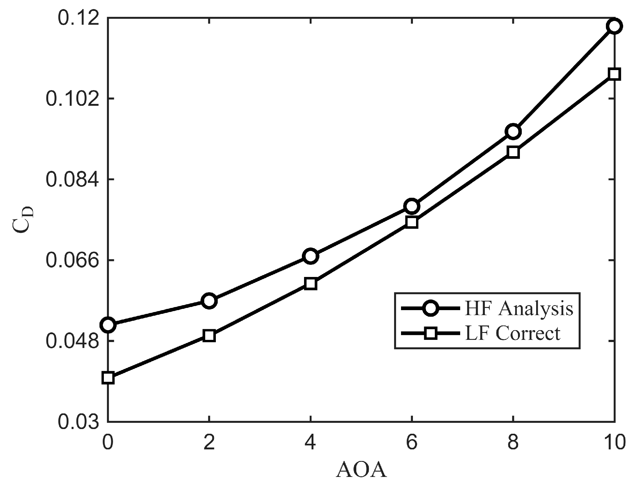
To further verify the effectiveness of the proposed drag estimation method, we consider the same geometric configuration and vary the angle of attack to generate a set of operating conditions. The corresponding corrected low-fidelity and high-fidelity drag coefficients and their comparison are shown in Figure A3.
The comparisons demonstrate that the corrected low-fidelity drag model yields satisfactory performance for subsequent multi-fidelity surrogate modeling and optimization.
Figure A3. The comparison between corrected low-fidelity and high-fidelity drag coefficients.
Drones 10 00290 g0a3

Appendix C. Neural Network Training Hyperparameters

To improve the reproducibility of the proposed active transfer learning framework, the main neural network training hyperparameters are summarized here according to the implementation used in this study.
(1)
Source domain pre-training
The source domain surrogate is a multilayer perceptron with the architecture Input-FC(64)-ReLU-Dropout(0.2)-FC(32)-ReLU-Dropout(0.2)-FC(16)-ReLU-FC. The model is trained using the Adam optimizer on a GPU with a mini-batch size of 16, a maximum of 80 epochs, and an initial learning rate of 0.01. A piecewise learning rate schedule is used, with a drop period of 100 epochs and a drop factor of 0.5. The L 2 regularization coefficient is set to 1 × 10 4 , and the training data are shuffled at every epoch.
(2)
Initial target domain fine-tuning
After transfer, the first two fully connected layers (fc1 and fc2) are frozen. The target domain model is then fine-tuned using Adam with a mini-batch size of 8, a maximum of 40 epochs, and an initial learning rate of 0.005. The same piecewise learning rate schedule is adopted, with a drop period of 80 epochs and a drop factor of 0.5.
(3)
Iterative active transfer stage
In the subsequent active learning iterations, the fc2 layer is gradually unfrozen. A dynamic dropout layer is inserted after relu2, with an initial dropout rate of 0.10. This dropout rate decays as
p drop = max ( 0.10 × 0 . 8 k ,   0.03 ) ,
where k = ( iter 1 ) / 3 . Meanwhile, the learning rate factor of the unfrozen fc2 layer is initialized as 0.1 and decays by a factor of two every three active learning iterations.
(4)
Custom optimization parameters
For the custom target network updating stage, the batch size is set to 12, the maximum number of epochs is 160, and the learning rate is 0.05. The optimizer uses first- and second-moment decay factors of 0.75 and 0.99, respectively.
(5)
Loss function weights
The transfer-related loss weights are set as follows: λ OT = 0.2 , λ Struct = 0.01 , λ Disent = 0.01 , with λ recon = 1 , λ confuse = 1 , and λ spec = 1 .
(6)
Uncertainty estimation
Monte Carlo stochastic forward inference is performed with T MC = 30 random forward passes. To improve robustness, a Gaussian perturbation with standard deviation 10 3 is added to the input during uncertainty evaluation.
(7)
Early stopping
No explicit early stopping strategy is used in the present implementation. Instead, training is terminated according to the predefined maximum number of epochs in each stage.

References

  1. Xu, C.; Yang, Y.; Kuang, M.; Zhuang, X.; Guo, H.; Han, Z.; Jia, L.; Zhu, J. Improved data-driven surrogate models by incorporating variable sensitivity for aerodynamic data modeling. Eng. Appl. Comput. Fluid Mech. 2025, 19, 2564830. [Google Scholar] [CrossRef]
  2. Leng, J.X.; Feng, Y.; Huang, W.; Shen, Y.; Wang, Z.G. Variable-fidelity surrogate model based on transfer learning and its application in multidisciplinary design optimization of aircraft. Phys. Fluids 2024, 36, 017131. [Google Scholar] [CrossRef]
  3. Esfahanian, V.; Izadi, M.J.; Bashi, H.; Ansari, M.; Tavakoli, A.; Kordi, M. Aerodynamic Shape Optimization of Gas Turbines: A Deep Learning Surrogate Model Approach. Struct. Multidiscip. Optim. 2024, 67, 2. [Google Scholar] [CrossRef]
  4. Espinosa Barcenas, O.U.; Quijada Pioquinto, J.G.; Kurkina, E.; Lukyanov, O. Multidisciplinary Analysis and Optimization Method for Conceptually Designing of Electric Flying-Wing Unmanned Aerial Vehicles. Drones 2022, 6, 307. [Google Scholar] [CrossRef]
  5. Wang, Y.; Huo, Y.; Zhong, Z.; Ji, R.; Chen, Y.; Wang, B.; Ma, X. A Robust Aerodynamic Design Optimization Methodology for UAV Airfoils Based on Stochastic Surrogate Model and PPO-Clip Algorithm. Drones 2025, 9, 607. [Google Scholar] [CrossRef]
  6. Wong, B.Y.J.; Damodaran, M.; Khoo, B.C. Physics-Informed Machine Learning Using Low-Fidelity Flowfields for Inverse Airfoil Shape Design. AIAA J. 2024, 62, 2846–2861. [Google Scholar] [CrossRef]
  7. Sun, Y.; Sengupta, U.; Juniper, M. Physics-informed Deep Learning for Simultaneous Surrogate Modeling and PDE-Constrained Optimization of an Airfoil Geometry. Comput. Methods Appl. Mech. Eng. 2023, 411, 116042. [Google Scholar] [CrossRef]
  8. Hai, C.; Mei, L. Hierarchical multi-fidelity surrogate modeling with curvature-and uncertainty-driven sampling for fluid flow prediction. Phys. Fluids 2025, 37, 097159. [Google Scholar] [CrossRef]
  9. Tao, J.; Sun, G. Application of Deep Learning Based Multi-Fidelity Surrogate Model to Robust Aerodynamic Design Optimization. Aerosp. Sci. Technol. 2019, 92, 722–737. [Google Scholar] [CrossRef]
  10. Le Gratiet, L. Bayesian Analysis of Hierarchical Multifidelity Codes. SIAM/ASA J. Uncertain. Quantif. 2013, 1, 244–269. [Google Scholar] [CrossRef]
  11. Han, Z.; Gortz, S.; Zimmermann, R. Hierarchical Kriging Model for Variable-fidelity Surrogate Modeling. AIAA J. 2012, 50, 1885–1896. [Google Scholar] [CrossRef]
  12. Zhang, M.; Jiao, J.; Zhang, J.; Zhang, Z. High-Efficiency Data Fusion Aerodynamic Performance Modeling Method for High-Altitude Propellers. Drones 2024, 8, 229. [Google Scholar] [CrossRef]
  13. Zhang, X.; Xie, F.; Ji, T.; Zhu, Z.; Zheng, Y. Multi-fidelity Deep Neural Network Surrogate Model for Aerodynamic Shape Optimization. Comput. Methods Appl. Mech. Eng. 2021, 373, 113485. [Google Scholar] [CrossRef]
  14. Meliani, M.; Bartoli, N.; Morlier, J.; Lefebvre, T.; Bouhlel, M.A.; Martins, J.R.R.A. Multi-fidelity Efficient Global Optimization: Methodology and Application to Airfoil Shape Design. In Proceedings of the AIAA AVIATION 2019 Forum, Dallas, TX, USA, 17–21 June 2019; AIAA: Reston, VA, USA, 2019; AIAA Paper 2019-3236. [Google Scholar] [CrossRef]
  15. Aye, C.M.; Wansaseub, K.; Kumar, S.; Tejani, G.G.; Bureerat, S.; Yildiz, A.R.; Pholdee, N. Airfoil Shape Optimisation Using a Multi-Fidelity Surrogate-Assisted Metaheuristic with a New Multi-Objective Infill Sampling Technique. CMES—Comput. Model. Eng. Sci. 2023, 137, 2111–2128. [Google Scholar] [CrossRef]
  16. Yang, A.; Li, J.; Liem, R.P. Multifidelity Data-driven Aerodynamic Shape Optimization of Wings with Composite Neural Networks. In Proceedings of the AIAA AVIATION 2023 Forum, San Diego, CA, USA, 12–16 June 2023; AIAA: Reston, VA, USA, 2023; AIAA Paper 2023-3470. [Google Scholar] [CrossRef]
  17. Pan, S.J.; Yang, Q. A Survey on Transfer Learning. IEEE Trans. Knowl. Data Eng. 2010, 22, 1345–1359. [Google Scholar] [CrossRef]
  18. Lu, D.; Ren, F.; Li, C.; Ming, H.; Cui, N. Fusing Coupled Degradation Mechanisms with Machine Learning: A Multi-fidelity Framework for Lithium-ion Battery Lifespan Prediction. Green Energy Intell. Transp. 2025, 5, 100367. [Google Scholar] [CrossRef]
  19. Settles, B. Active Learning Literature Survey; Technical Report 1648; Computer Sciences Department, University of Wisconsin–Madison: Madison, WI, USA, 2009. [Google Scholar]
  20. Ren, P.; Xiao, Y.; Chang, X.; Huang, P.; Li, Z.; Chen, X.; Wang, X.; Zhang, X. A Survey of Deep Active Learning. ACM Comput. Surv. 2021, 54, 1–40. [Google Scholar] [CrossRef]
  21. Ghazi, Y.; Alhazmi, N.; Tezaur, R.; Farhat, C. Training a Neural-Network-Based Surrogate Model for Aerodynamic Optimisation Using a Gaussian Process. Int. J. Comput. Fluid Dyn. 2022, 36, 538–554. [Google Scholar] [CrossRef]
  22. Liu, J.; Jiang, Y.; Tao, J.; Wu, G. Aerodynamic Shape Optimization via Active Learning-Driven Design Space Refinement. Aerosp. Sci. Technol. 2025, 166, 110606. [Google Scholar] [CrossRef]
  23. Wang, K.; Zhang, D.; Li, Y.; Zhang, R.; Lin, L. Cost-Effective Active Learning for Deep Image Classification. IEEE Trans. Circuits Syst. Video Technol. 2016, 27, 2591–2600. [Google Scholar] [CrossRef]
  24. Zhang, Y.; Zheng, X.; Gong, Z.; Yao, W.; Zhao, X. Towards sparse sensor annotations: Uncertainty-based active transfer learning for airfoil flow field prediction. Chin. J. Aeronaut. 2024, 37, 87–98. [Google Scholar] [CrossRef]
  25. Garbo, A.; Parekh, J.; Rischmann, T.; Bekemeyer, P. Multi-Fidelity Adaptive Sampling for Surrogate-Based Optimization and Uncertainty Quantification. Aerospace 2024, 11, 448. [Google Scholar] [CrossRef]
  26. Do, B.; Zhang, R. Multifidelity Bayesian Optimization: A Review. AIAA J. 2025, 63, 2286–2322. [Google Scholar] [CrossRef]
  27. Veiga-Piñeiro, G.; Aldao-Pensado, E.; Martín-Ortega, E. Hybrid CFD-Deep Learning Approach for Urban Wind Flow Predictions and Risk-Aware UAV Path Planning. Drones 2025, 9, 791. [Google Scholar] [CrossRef]
  28. Damianou, A.; Lawrence, N.D. Deep Gaussian Processes. In Proceedings of the 16th International Conference on Artificial Intelligence and Statistics (AISTATS); Proceedings of Machine Learning Research; PMLR: New York, NY, USA, 2013; Volume 31, pp. 207–215. [Google Scholar]
  29. Neal, R.M. Bayesian Learning for Neural Networks; Lecture Notes in Statistics; Springer: Berlin/Heidelberg, Germany, 1996; Volume 118. [Google Scholar] [CrossRef]
  30. Devlin, J.; Chang, M.W.; Lee, K.; Toutanova, K. BERT: Pre-training of Deep Bidirectional Transformers for Language Understanding. In Proceedings of the 2019 Conference of the North American Chapter of the Association for Computational Linguistics: Human Language Technologies (NAACL-HLT); Association for Computational Linguistics: Stroudsburg, PA, USA, 2019; Volume 1, pp. 4171–4186. [Google Scholar]
  31. McKay, M.D.; Beckman, R.J.; Conover, W.J. A Comparison of Three Methods for Selecting Values of Input Variables in the Analysis of Output from a Computer Code. Technometrics 1979, 21, 239–245. [Google Scholar] [CrossRef] [PubMed]
  32. Gal, Y.; Ghahramani, Z. Dropout as a Bayesian Approximation: Representing Model Uncertainty in Deep Learning. In Proceedings of the 33rd International Conference on Machine Learning (ICML); Proceedings of Machine Learning Research; PMLR: New York, NY, USA, 2016; Volume 48, pp. 1050–1059. [Google Scholar]
  33. Kullback, S.; Leibler, R.A. On Information and Sufficiency. Ann. Math. Stat. 1951, 22, 79–86. [Google Scholar] [CrossRef]
  34. Gretton, A.; Borgwardt, K.M.; Rasch, M.J.; Schölkopf, B.; Smola, A. A Kernel Two-Sample Test. J. Mach. Learn. Res. 2012, 13, 723–773. [Google Scholar]
  35. Ganin, Y.; Lempitsky, V. Unsupervised domain adaptation by backpropagation. J. Mach. Learn. Res. 2015, 17, 1–35. [Google Scholar]
  36. Forrester, A.I.J.; Sóbester, A.; Keane, A.J. Multi-fidelity optimization via surrogate modelling. Proc. R. Soc. A 2007, 463, 3251–3269. [Google Scholar] [CrossRef]
  37. Kulfan, B.M. Universal Parametric Geometry Representation Method. J. Aircr. 2007, 45, 142–158. [Google Scholar] [CrossRef]
  38. Yang, D.; Liu, L.; Bai, W.; Tian, W. Conceptual design and configurations selection of S/H-UAVs based on Q-rung dual hesitant double layer FQFD. Chin. J. Aeronaut. 2024, 37, 193–205. [Google Scholar] [CrossRef]
  39. Grasmeyer, J. Truss-Braced Wing Code Description and User’s Manual; Technical Report VPI-AOE-255; Department of Aerospace and Ocean Engineering, Virginia Polytechnic Institute and State University: Blacksburg, VA, USA, 1998. [Google Scholar]
  40. Gur, O.; Mason, W.H.; Schetz, J.A. Full-Configuration Drag Estimation. J. Aircr. 2010, 47, 1356–1367. [Google Scholar] [CrossRef]
  41. Hoerner, S.F. Fluid-Dynamic Drag; Hoerner Fluid Dynamics: Vancouver, WA, USA, 1965. [Google Scholar]
  42. Raymer, D.P. Aircraft Design: A Conceptual Approach; American Institute of Aeronautics and Astronautics (AIAA): Washington, DC, USA, 1992. [Google Scholar]
Figure 1. Framework of the proposed active transfer learning multi-fidelity surrogate model.
Drones 10 00290 g001
Figure 2. Low and high fidelity of Forrester’s function.
Drones 10 00290 g002
Figure 3. Baseline and design area of the NACA0012 case.
Drones 10 00290 g003
Figure 4. The configuration of the UAV with strut-braced wing.
Drones 10 00290 g004
Figure 5. Result comparison of different algorithms with Forrester’s function.
Drones 10 00290 g005
Figure 6. Model performance indicators under 20 calculation conditions.
Drones 10 00290 g006
Figure 7. Workflow and dataflow of multi-fidelity analysis.
Drones 10 00290 g007
Figure 8. CFD airfoil mesh adopted for the high-fidelity simulations.
Drones 10 00290 g008
Figure 9. Result comparison of different algorithms in airfoil aerodynamic analysis.
Drones 10 00290 g009
Figure 10. Result comparison of different algorithms in UAV aerodynamic analysis.
Drones 10 00290 g010
Figure 11. The impact of MMD loss on performance.
Drones 10 00290 g011
Figure 12. The impact of structural loss on performance.
Drones 10 00290 g012
Figure 13. The impact of feature decoupling loss on performance.
Drones 10 00290 g013
Figure 14. The impact of uncertainty weight on performance.
Drones 10 00290 g014
Figure 15. The impact of diversity weight on performance.
Drones 10 00290 g015
Figure 16. The impact of KL divergence weight on performance.
Drones 10 00290 g016
Figure 17. Bar comparison of performance indicators and computation time.
Drones 10 00290 g017
Table 1. Network architectures of source and target domains.
Source NetOperationTarget Net
Input Layer Input Layer
Fully Connection Layer (64)→Freeze→Fully Connection Layer (64)
ReLu ReLu
Dropout LayerDelete Dropout Layer↓Connect
Fully Connection Layer (32)→Gradually unfreeze→Fully Connection Layer (32)
ReLu ReLu
Dropout LayerUpdated Dropout Layer↓Adaptively updated
Fully Connection Layer (16)→Gradually unfreeze→Fully Connection Layer (16)
ReLu ReLu
Fully Connection Layer (num of feature) Fully Connection Layer (of feature)
Table 2. Introduction to comparative algorithms.
AlgorithmActive Learning SamplingGPR-AssistedTransfer TrainingLoss Function
Method 1 (MSE Loss)Random sampling/Standard trainingMSE
Method 2 (MSD Loss)Random sampling/Transfer learningMSD
Method 3 (ATL without GPR)Active sampling/Transfer learningMSD
Method 4 (ATL with GPR)Active samplingTransfer learningMSD
Method 5 (HK)////
Table 3. Design variables and bounds for the SBW UAV aerodynamic analysis.
IndexDesign VariableDescriptionLower BoundsUpper Bounds
1bMain-wing span (m)6.010.0
2 b sbw SBW spanwise length (m)2.06.0
3 L sbw SBW bottom length (m)0.42.0
4 h pyl Pylon/strut height (m)0.040.20
5 l tail Tail moment arm (m)1.53.0
6 b ht Horizontal-tail span (m)0.81.5
7 h vt Vertical-tail height (m)0.30.6
Table 4. Performance indicators and computation time under different conditions.
ATL Without GPRATL with GPR
Number of Candidate Pool Points308020020
R 2 0.9310.9540.9860.965
Computation time345 s401 s530 s356 s
Disclaimer/Publisher’s Note: The statements, opinions and data contained in all publications are solely those of the individual author(s) and contributor(s) and not of MDPI and/or the editor(s). MDPI and/or the editor(s) disclaim responsibility for any injury to people or property resulting from any ideas, methods, instructions or products referred to in the content.