Active Acoustic Sensing of Ground Surface Condition Using a Drone-Mounted Speaker–Microphone Array

Highlights

What are the main findings?

• A MUSIC-based active acoustic sensing framework using a drone-mounted speaker-microphone array is proposed, demonstrating the capability to detect ground surface anomalies such as depressions and cracks, and clarifying its fundamental performance and sensing coverage.
• The simultaneous execution of active acoustic sensing and sound source localization (SSL) for victim search in search and rescue (SAR) missions is experimentally evaluated, and the conditions under which both tasks can be effectively performed are identified.

What are the implications of the main findings?

• The proposed framework enables ground surface sensing and victim search to share hardware and signal processing components on a single drone platform without increasing system complexity.
• A fundamental trade-off between active acoustic sensing and SSL performance is revealed, highlighting the necessity of joint optimization of sensing signal design and drone operation in practical SAR missions.

Abstract

Rapid assessment of ground surface conditions is essential in disaster response and search-and-rescue operations, where drones are increasingly deployed for aerial inspection and victim localization. This paper proposes an active acoustic sensing method for estimating ground surface conditions using a drone-mounted speaker and microphone array. The method is based on the multiple signal classification framework and enables three-dimensional localization of reflection points according to the principle of echolocation. A key feature of the proposed approach is that it shares both hardware and signal processing components with acoustic-based victim search, allowing simultaneous execution of surface sensing and sound source localization (SSL) on a single drone platform without increasing system complexity. Outdoor experiments were conducted to evaluate sensing performance for ground surface anomalies, specifically ground surface depressions and cracks. The experimental results clarify the achievable sensing performance and coverage in real environments and reveal key factors affecting detection performance. The feasibility of simultaneous execution of active acoustic sensing and SSL was also investigated, and the mutual interactions between sensing and localization performance were clarified. These findings highlight both the potential and the practical limitations of integrating environmental sensing and victim localization on a single drone platform.

1. Introduction

Natural disasters such as earthquakes, landslides, floods, and large-scale urban collapses occur frequently worldwide and often result in severe human casualties and extensive damage to infrastructure. For example, the 2023 Türkiye–Syria earthquake caused more than fifty thousand fatalities [1,2], highlighting the devastating impact of large-scale disasters and the urgent need for effective response strategies. In such situations, search and rescue (SAR) operations play a crucial role in saving lives, as the survival probability of trapped victims strongly depends on the speed and effectiveness of rescue activities. It is widely recognized that survival rates decrease significantly after approximately 72 h following a disaster, a period commonly referred to as the “Golden 72 h” [3], emphasizing the importance of prompt victim detection and situational awareness during SAR operations.

Traditionally, SAR operations have relied heavily on human responders and trained rescue dogs to search for and locate trapped or buried victims. While these approaches have been widely used in many disaster scenarios, they often suffer from limited search efficiency and incomplete coverage, resulting in difficulties in reliably locating all trapped victims within a limited time window. In addition, these operations impose a high physical burden on responders and involve significant safety risks, particularly in unstable or hazardous environments such as collapsed buildings or landslide areas. These limitations have motivated extensive research into robotic technologies for SAR, aiming to support or replace human responders in dangerous or inaccessible locations. Various types of disaster-response robots have been developed and deployed for SAR applications [4,5]. For example, ground-based mobile robots have been designed to navigate through debris-filled environments and provide information about trapped victims and surrounding conditions to support rescue operations [6]. In addition, snake-like or articulated robots have been proposed to penetrate narrow voids and confined spaces where conventional robots or human rescuers cannot enter [7]. These robotic systems have demonstrated the potential to enhance situational awareness while reducing the risk to human rescuers.

Among these robotic platforms, unmanned aerial vehicles (UAVs), commonly referred to as drones, have attracted increasing attention in recent years [8]. Unlike ground-based robots, drones can be rapidly deployed without requiring ground access routes, enabling immediate observation of large-scale disaster areas. Their ability to operate above rubble, flooded regions, or collapsed infrastructure allows for efficient wide-area surveillance and information collection. As a result, drones have become an essential tool in modern SAR operations, complementing ground-based robotic systems and human rescue teams in post-disaster environments. Most existing drone-based SAR systems primarily depend on vision-based sensing [9,10,11]. While vision-based approaches are effective under favorable conditions, they face inherent difficulties in low-visibility environments, such as darkness, smoke, dust, or adverse weather conditions. Moreover, they are fundamentally limited when victims are buried under rubble or debris and are not directly visible. Historical disaster records indicate that a large proportion of fatalities were caused by people being trapped or crushed under collapsed structures [12,13], underscoring the need for sensing modalities that do not rely solely on visual information.

To address these limitations of vision-based approaches, acoustic-based victim search using drones has been studied. By mounting microphones on drones, it becomes possible to detect human-related sounds, such as voices, or emergency whistles, even when visual information is unavailable. In this research area, referred to as “drone audition”, sound source localization (SSL) and sound source separation/enhancement (SSS/SSE) are often addressed. A comprehensive review of drone audition technologies is presented by Chevtchenko et al. [14]. For example, Hoshiba et al. proposed an SSL method based on multiple signal classification (MUSIC) [15] to localize a sound source on the ground using a spherical microphone array mounted on the front of a drone [16,17,18]. Wang et al. mounted a microphone array to the top of a drone and proposed a deep neural network (DNN)-based speech enhancement method [19]. Strauss et al. produced and published a dataset of acoustic signals recorded via a drone-embedded microphone array to advance drone audition research [20]. These studies have shown that acoustic sensing can complement vision-based methods and significantly enhance SAR capabilities in challenging environments. However, existing acoustic-based SAR studies have primarily focused on localizing victims, aiming to estimate the direction or position of sound sources. In practical SAR scenarios, locating victims alone is not sufficient. Rescue teams must also understand the surrounding environment, including ground surface conditions, debris distribution, and potential hazards, in order to determine safe rescue routes and appropriate rescue strategies. The lack of information about ground surface conditions can lead to inefficient rescue planning or even secondary accidents. Therefore, acquiring environmental information around victims, in addition to their estimated locations, is essential for effective and safe SAR operations.

In parallel with victim detection and localization, environmental sensing using drones has been widely studied to acquire information about disaster environments. In particular, vision-based sensing using RGB cameras and LiDAR (Light Detection and Ranging)-based mapping techniques have been widely employed to reconstruct three-dimensional structures of damaged areas, assess terrain geometry, and identify obstacles or hazardous regions. For example, Cheng et al. propose a method for reconstructing three-dimensional land surfaces using sequential images captured by a drone-mounted camera [21]. Suzuki et al. developed a drone equipped with a LiDAR sensor and multiple GNSS (Global Navigation Satellite System) antennas and generated a three-dimensional map [22]. Such techniques have shown strong potential for applications including infrastructure inspection, terrain assessment, and navigation planning in disaster-response scenarios. However, these environmental sensing approaches are predominantly reliant on visual or laser-based sensing modalities, which inherently suffer from several limitations in SAR contexts. Vision-based sensing is vulnerable to poor visibility caused by darkness, smoke, dust, or adverse weather conditions, as in vision-based victim search. In addition, vision-based sensing often provides limited accuracy in the vertical direction, making it difficult to reliably capture height variations and subtle surface irregularities of the ground. While LiDAR-based approaches can provide more accurate geometric measurements, their performance may be degraded by reflective surfaces or occlusions in cluttered environments. Moreover, both vision- and LiDAR-based approaches often require the deployment of multiple sensors, which increases payload weight, power consumption, and system complexity of drones. Although these issues could be alleviated by using multiple drones equipped with different sensors, such configurations tend to reduce real-time capabilities and operational efficiency. This limitation becomes particularly critical in time-sensitive SAR missions, where rapid and integrated situational awareness is required. Therefore, there is a need for a novel sensing modality that can be used simultaneously with acoustic-based victim search to provide complementary environmental information, without imposing additional hardware or operational burdens. In addition to these vision- and LiDAR-based approaches, acoustic-based environmental sensing has also been investigated. For example, Afriansyah et al. and Su et al. developed drone systems that use ultrasonic sensors to measure the distance between the drone and the ground surface for navigation purposes [23,24]. However, these systems are primarily designed for altitude measurement and provide limited information about surrounding environments. Moreover, ultrasonic sensing requires dedicated transmitters and receivers operating in a different frequency range from those used for acoustic victim search, which increases system complexity. Other studies have explored environmental sensing using drone ego-noise. For example, Nilsson et al., Wilshin et al., and Yano et al. proposed sensing systems that utilize drone-generated acoustic noise to detect obstacles, other drones, or surface materials [25,26,27]. Since these approaches operate in a similar frequency range to that used for acoustic victim search, they have the advantage that sensing hardware can potentially be shared. However, these systems mainly focus on obstacle detection or situational awareness and do not explicitly address detailed sensing of ground surface structures. Furthermore, recent studies have actively investigated techniques for reducing drone ego-noise [28]. As drone noise levels decrease, the performance of sensing methods relying on ego-noise may also be degraded. Therefore, there is a need for a sensing method that can perform environmental sensing while sharing hardware and signal processing with acoustic victim search, without relying on drone ego-noise. In practical SAR operations, sensing systems must also satisfy strict operational constraints. Sensors mounted on drones should be compact and lightweight to ensure rapid deployment and stable flight performance. Large or complex sensing systems increase payload weight and may degrade flight stability, which can limit operational efficiency in disaster environments. Therefore, developing sensing methods that can operate with compact sensor configurations while maintaining practical sensing capability is an important requirement for drone-based SAR systems.

In this paper, we propose an active acoustic sensing method for ground surface condition estimation that can be performed simultaneously with acoustic-based victim search using a single drone platform. The proposed approach relies primarily on a drone-mounted speaker and a microphone array. By actively emitting acoustic signals from the speaker and analyzing the reflected signals from the ground surface, the method estimates both the propagation time and the direction of arrival (DOA) of the reflected signals using a MUSIC-based algorithm. This enables the three-dimensional localization of reflection points, allowing spatial sensing of ground surface conditions based on the principle of echolocation. The proposed method is designed to share both the microphone array and the MUSIC-based signal processing framework with acoustic-based victim search. This commonality allows the hardware configuration and signal processing pipeline to be simplified. The proposed framework is expected to enable the simultaneous execution of victim localization and ground surface condition estimation using a single drone platform, without increasing system complexity. Active acoustic sensing of surrounding conditions in indoor or outdoor environments has been reported in various studies [29,30,31,32,33], demonstrating its potential for extracting environmental information from acoustic reflections. These findings suggest that the proposed drone-based active acoustic sensing framework is a promising approach for acquiring environmental information around victims in SAR scenarios. The remainder of this paper is organized as follows: Section 2 describes the SSL and active acoustic sensing methods. Section 3 evaluates and discusses the performance of the proposed method and the potential of simultaneous execution of victim localization and ground surface condition estimation through numerical simulations and real outdoor experiments. Section 4 presents the conclusions.

2. Methods

This section describes the SSL method used for acoustic-based victim search and the proposed active acoustic sensing method for ground surface condition estimation.

2.1. Sound Source Localization Method

In this study, SSL is performed using a MUSIC-based method, SEVD-MUSIC (MUSIC based on Standard EigenValue Decomposition) [15], adopted in our previous studies. The algorithm is described below.

The M-channel acoustic input signal, $x(t,m)$, is transformed into the frequency domain by applying the short-time Fourier transform (STFT), resulting in $Z(\omega ,f,m)$, where $\omega$ denotes the frequency bin index, f denotes the frame number, and m denotes the channel number. Based on $Z(\omega ,f,m)$, the correlation matrix $R(\omega ,f)$ is defined as

$$R(\omega ,f)={\displaystyle \frac{1}{T_R}}\sum _{\tau =f}^{f+T_R-1}{\left\{Z(\omega ,\tau ,m)\right\}}_m{\left\{Z^{*}(\omega ,\tau ,m)\right\}}_m.$$

(1)

Here, $T_R$ represents the number of frames used for temporal averaging of the correlation matrix, ${(·)}^{*}$ denotes the complex conjugate transpose, and ${\left\{Z(\omega ,\tau ,m)\right\}}_m$ denotes an M-dimensional column vector whose elements are $Z(\omega ,\tau ,m)$ for $m=1,\dots ,M$. In SEVD-MUSIC, the eigenvectors are obtained by performing eigenvalue decomposition of the correlation matrix $R(\omega ,f)$ as

$$R(\omega ,f)=E(\omega ,f)\Lambda (\omega ,f)E^{*}(\omega ,f).$$

(2)

In this formulation, $\Lambda (\omega ,f)$ is a diagonal matrix whose elements are eigenvalues sorted in descending order, and $E(\omega ,f)$ consists of the corresponding eigenvectors. The correlation matrix $R(\omega ,f)$ is thus decomposed into signal and noise subspaces through eigenvalue decomposition. The MUSIC algorithm exploits the orthogonality between the array manifold vector corresponding to the signal direction and the noise subspace. Using the array manifold vector $G(\omega ,\psi )$, which represents the transfer function from a sound source at direction $\psi$ to each microphone, and the eigenvectors corresponding to the noise subspace, the MUSIC spatial spectrum $P(\omega ,\psi ,f)$ is calculated as

$$P(\omega ,\psi ,f)={\displaystyle \frac{|G^{*}(\omega ,\psi )G(\omega ,\psi )|}{{\sum }_{m=L+1}^M\left|G^{*}(\omega ,\psi )e_m(\omega ,f)\right|}}.$$

(3)

Here, L denotes the assumed number of sound sources, and $e_m(\omega ,f)$ is the m-th eigenvector corresponding to the noise subspace. The direction parameter $\psi$ is defined as $\psi =(\theta ,\varphi )$, where $\theta$ and $\varphi$ indicate the azimuth and elevation angles in the drone coordinate system, respectively. When the candidate direction $\psi$ coincides with the true sound source direction, the array manifold vector becomes orthogonal to the noise subspace, causing the denominator of Equation (3) to approach zero and producing a sharp peak in the spatial spectrum. Therefore, the DOA can be estimated by scanning $\psi$ and identifying the peak of the spatial spectrum. To enhance robustness, the spatial spectrum is integrated over a predefined frequency range as

$$\overline{P}(\psi ,f)=\sum _{\omega ={\omega }_L}^{{\omega }_H}P(\omega ,\psi ,f)$$

(4)

Here, ${\omega }_L$ and ${\omega }_H$ correspond to the lower and upper frequency bin indices used in the summation. Both $P(\omega ,\psi ,f)$ and $\overline{P}(\psi ,f)$ represent the power of the sound arriving from direction $\psi$ at frame f. Finally, the target sound direction ${\psi }_{target}$ is estimated by identifying the peak of the integrated spatial spectrum as

$${\psi }_{target}\left(f\right)=\underset{\psi }{\mathrm{argmax}}\left(\overline{P}(\psi ,f)\right).$$

(5)

2.2. Active Acoustic Sensing Method

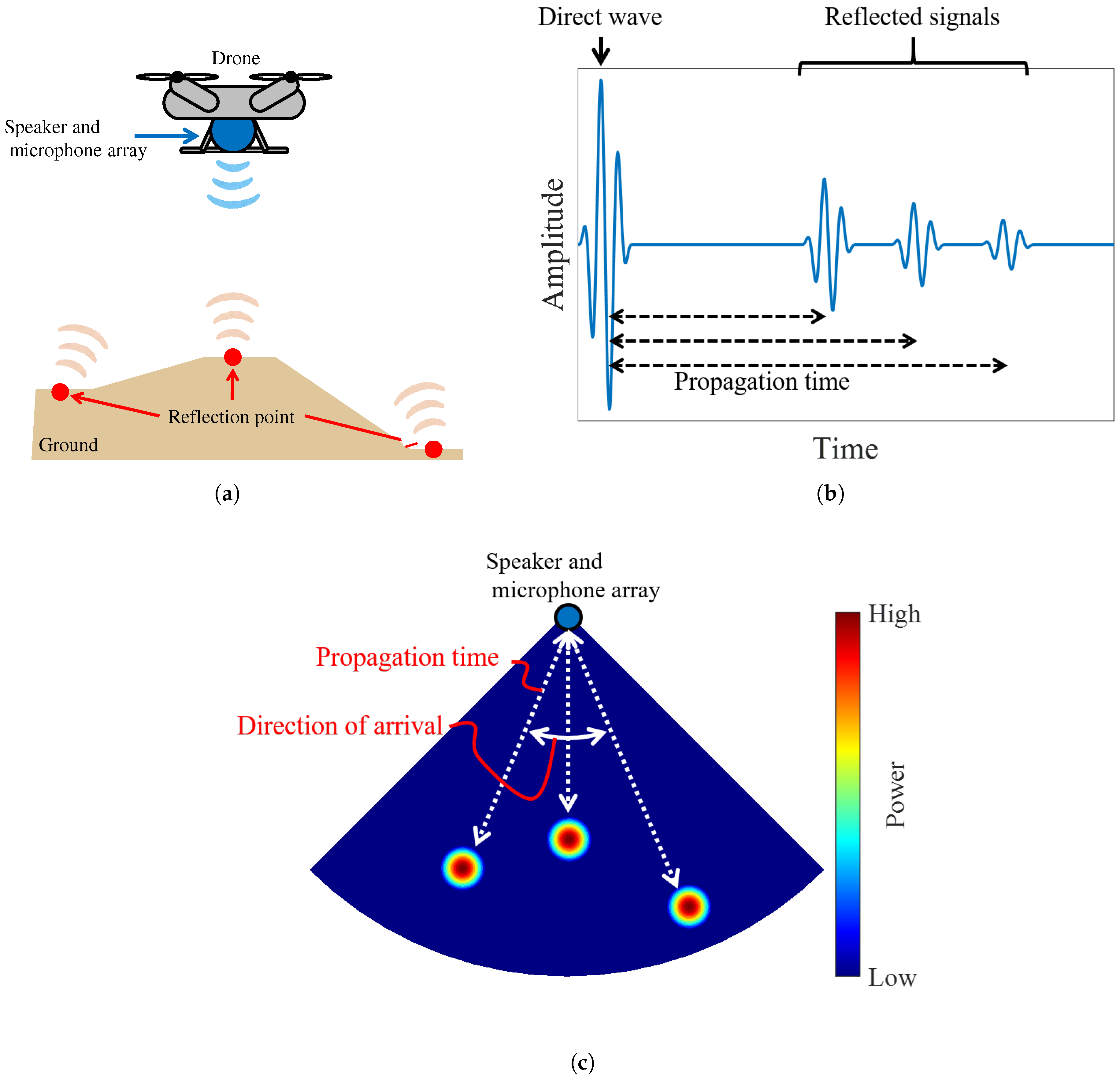
Next, the proposed active acoustic sensing method based on the MUSIC framework is described. Figure 1 illustrates the conceptual overview of the proposed approach. In this method, a speaker and a microphone array are mounted on a drone platform. As shown in Figure 1a, acoustic signals emitted from the onboard speaker toward the ground surface are reflected at multiple points on the ground, and the resulting reflected signals are recorded by the microphone array. An example of the recorded signals is shown in Figure 1b. The recorded signals consist of a direct wave that propagates directly from the speaker to the microphone array, as well as reflected signals originating from individual reflection points on the ground surface. The time difference between the arrival of the direct wave and each reflected signal corresponds to the propagation time of the reflected path, from which the propagation distance can be estimated. Furthermore, by estimating the DOA of each reflected signal, the three-dimensional positions of the reflection points can be determined from the estimated propagation distances and directions, enabling three-dimensional sensing of ground surface conditions. The details of the algorithm are described below.

In the previous subsection, $Z(\omega ,f,m)$ is calculated using the STFT, and the DOA is estimated using the MUSIC method. As a result, the DOA estimation is performed on a frame-by-frame basis, as shown in Equation (4). For example, in our previous studies, the DOA was estimated at intervals of 0.5 s. However, in the proposed method, it is necessary to estimate the propagation distance from the propagation time. Therefore, frame-based DOA estimation, as described in the previous subsection, significantly degrades the distance resolution. To address this issue, the proposed method applies quadrature demodulation [34] to obtain a complex-valued signal $Z^{\prime }(\omega ,t,m)$ as

$$Z^{\prime }(\omega ,t,m)={\mathrm{LPF}}_{\omega }\left(x(t,m)e^{-j\omega t}\right).$$

(6)

Here, ${\mathrm{LPF}}_{\omega }(·)$ denotes a low-pass filter with a cutoff frequency of $\omega$. This quadrature demodulation in Equation (6) is performed for the frequencies analyzed in this study, i.e., for the frequency range from ${\omega }_L$ to ${\omega }_H$ used in Equation (4). By applying this processing, complex-valued signals containing both amplitude and phase information, equivalent to those obtained from the STFT, can be obtained at the time-sample level. This enables the arrival time of reflected signals to be analyzed with sample-level resolution, allowing the propagation distance to be estimated with higher accuracy. Subsequently, following Equations (1)–(4), the correlation matrix $R^{\prime }(\omega ,t)$, the eigenvalues and eigenvectors ${\Lambda }^{\prime }(\omega ,t)$ and $E^{\prime }(\omega ,t)$, the MUSIC spatial spectrum $P^{\prime }(\omega ,\psi ,t)$, and the frequency-integrated spatial spectrum $\overline{P^{\prime }}(\psi ,t)$ are calculated as

$$R^{\prime }(\omega ,t)={\displaystyle \frac{1}{t_R}}\sum _{\tau =t}^{t+t_R-1}{\left\{Z^{\prime }(\omega ,\tau ,m)\right\}}_m{\left\{Z^{\prime *}(\omega ,\tau ,m)\right\}}_m,$$

(7)

$$R^{\prime }(\omega ,t)=E^{\prime }(\omega ,t){\Lambda }^{\prime }(\omega ,t)E^{\prime *}(\omega ,t),$$

(8)

$$P^{\prime }(\omega ,\psi ,t)={\displaystyle \frac{|G^{*}(\omega ,\psi )G(\omega ,\psi )|}{{\sum }_{m=L+1}^M\left|G^{*}(\omega ,\psi )e_m^{\prime }(\omega ,t)\right|}},$$

(9)

$$\overline{P^{\prime }}(\psi ,t)=\sum _{\omega ={\omega }_L^{\prime }}^{{\omega }_H^{\prime }}{P}^{\prime }(\omega ,\psi ,t).$$

(10)

Here, $t_R$ denotes the number of time samples used for temporal averaging of the correlation matrix, $e_m^{\prime }(\omega ,t)$ represents the m-th eigenvector corresponding to the noise subspace, and ${\omega }_L^{\prime }$ and ${\omega }_H^{\prime }$ denote the lower and upper frequency limits used in the summation, respectively. In this manner, a spatial spectrum is obtained on a time-sample basis.

A conceptual illustration of the resulting spatial spectrum $\overline{P^{\prime }}(\psi ,t)$ is shown in Figure 1c. For simplicity, the spatial spectrum is illustrated in two dimensions, although $\overline{P^{\prime }}(\psi ,t)$ is obtained as a three-dimensional distribution. When the origin of the fan-shaped representation is defined as the position of the speaker and the microphone array, the radial direction corresponds to the propagation time t, while the angular direction represents the DOA $\psi$, and the power of each reflected signal is mapped accordingly. That is, the presence of reflection points can be inferred from regions with high power in the spatial spectrum. Finally, by converting the spatial spectrum into a Cartesian coordinate representation $\overline{P^{\prime }}(x,y,z)$ using the speed of sound and the coordinates of the speaker and microphone array, three-dimensional sensing of ground surface conditions is achieved. In this paper, the frequency-integrated MUSIC spatial spectrum $\overline{P^{\prime }}(x,y,z)$ is used as the sensing result for ground surface condition estimation.

In acoustic sensing, conventional methods such as synthetic aperture techniques [35] provide a theoretical beamwidth (i.e., angular resolution) given by $\lambda /D$, where $\lambda$ is the wavelength of the transmitted signal and D is the aperture size of the sensor array. In contrast, the MUSIC algorithm employed in this study is a subspace-based method for high-resolution direction estimation, which can provide higher resolution than conventional synthetic aperture techniques under favorable conditions. As shown in Equation (9), when the transfer function perfectly matches the received signal under ideal conditions, the denominator becomes zero, and the MUSIC spatial spectrum theoretically diverges at the direction of the reflected signal. As a result, the spectrum exhibits an infinitely sharp peak, corresponding to ideal (i.e., theoretically zero) angular resolution. However, in practical environments, the angular resolution is limited by various factors, such as noise, variations in the speed of sound, position errors of the speaker and microphones, and synchronization inaccuracies in transmission and reception. These factors cause the peak of the MUSIC spatial spectrum to have a finite width. Therefore, in this study, the effective angular and range (i.e., distance) resolutions are defined based on the full width at half maximum (FWHM) of the peaks in the MUSIC spatial spectrum, to quantitatively evaluate the practical sensing performance.

3. Evaluation Experiments and Discussion

In this section, the performance of the proposed active acoustic sensing method alone and the potential for its simultaneous execution with SSL are evaluated through numerical simulations and real outdoor experiments.

3.1. Evaluation of Active Acoustic Sensing Performance

3.1.1. Experimental Setup

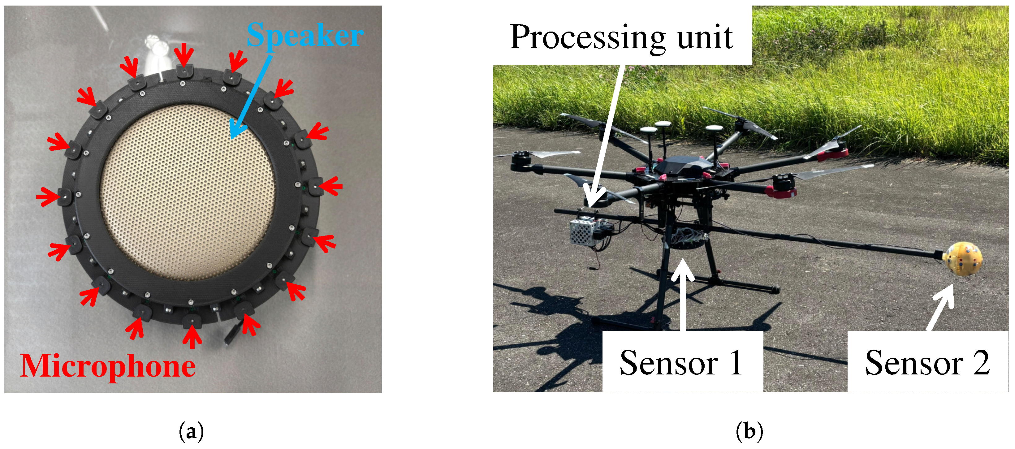
To evaluate the intrinsic performance of the proposed active acoustic sensing method independently of SSL, sensing experiments were conducted in a real outdoor environment under stable weather conditions. Figure 2a shows the integrated speaker–microphone array sensor used in the experiments (Sensor 1). In Sensor 1, a speaker is placed at the center, and 16 microphones are arranged uniformly on a circular array with a diameter of 155 mm around the speaker. The diameter of the microphone array is intentionally designed to be compact so that the sensing system can be easily mounted on a drone platform without significantly affecting flight stability. In practical SAR operations, sensing systems should be lightweight and mechanically simple to allow rapid deployment and stable flight performance in complex disaster environments. Large or heavy sensing systems increase payload weight and may degrade flight stability or operational flexibility. Therefore, the proposed sensing system employs a compact circular array configuration that can be readily integrated with drone-based victim search systems. Investigating the sensing capability achievable with such compact arrays is an important step toward developing practical drone-based sensing systems. As shown in Figure 2b, Sensor 1 is mounted downward on the lower part of the drone. In addition, a processing unit for signal recording and transmission to the ground station is installed on a pipe attached to the drone. A Matrice 600 Pro drone (DJI, Shenzhen, China) is used as the drone platform. The same pipe also carries a microphone array (Sensor 2) that has been used in previous drone audition studies for victim search and is employed in the evaluation of simultaneous execution with SSL. Details of Sensor 2 are described in Section 3.2. In the experiments, a chirp signal is transmitted from the speaker of Sensor 1 toward the ground surface to improve the signal-to-noise ratio (SNR) of reflected signals relative to drone ego-noise. The reflected signals from the ground surface are synchronously recorded at each channel with a sampling frequency of 48 kHz and a quantization resolution of 24 bit. The recorded signals are processed using pulse compression [36], and the resulting signals are analyzed using the proposed method.

Although simulation-based analysis is useful for investigating acoustic sensing performance and array configurations, accurately modeling acoustic reflections and environmental noise in complex outdoor disaster environments is challenging. Therefore, this study first focuses on experimental validation in a real outdoor environment in order to investigate the practical sensing characteristics and identify potential issues of the proposed method. Simulation-based analyses will be conducted in future work based on the insights obtained from these experimental results.

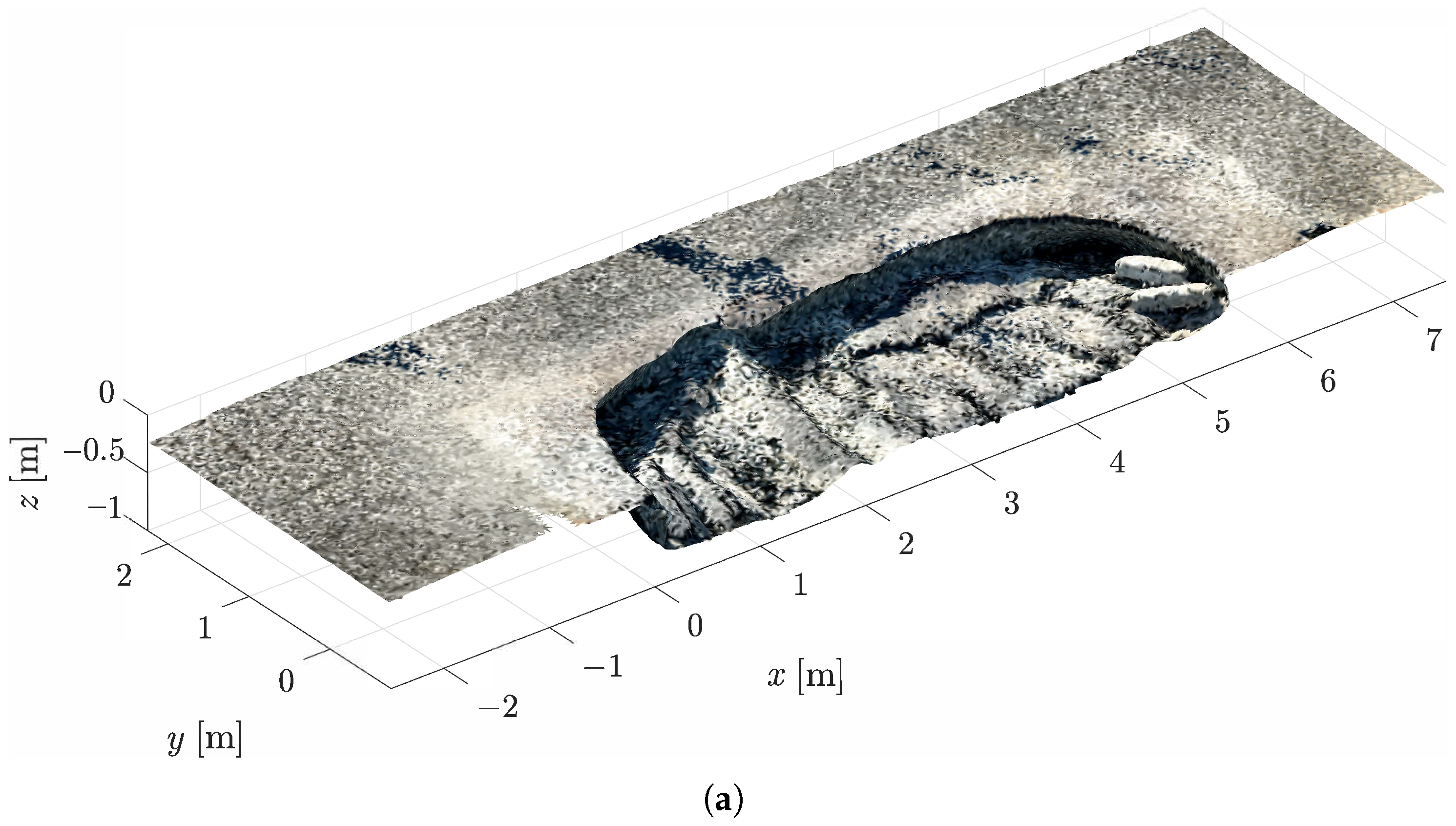
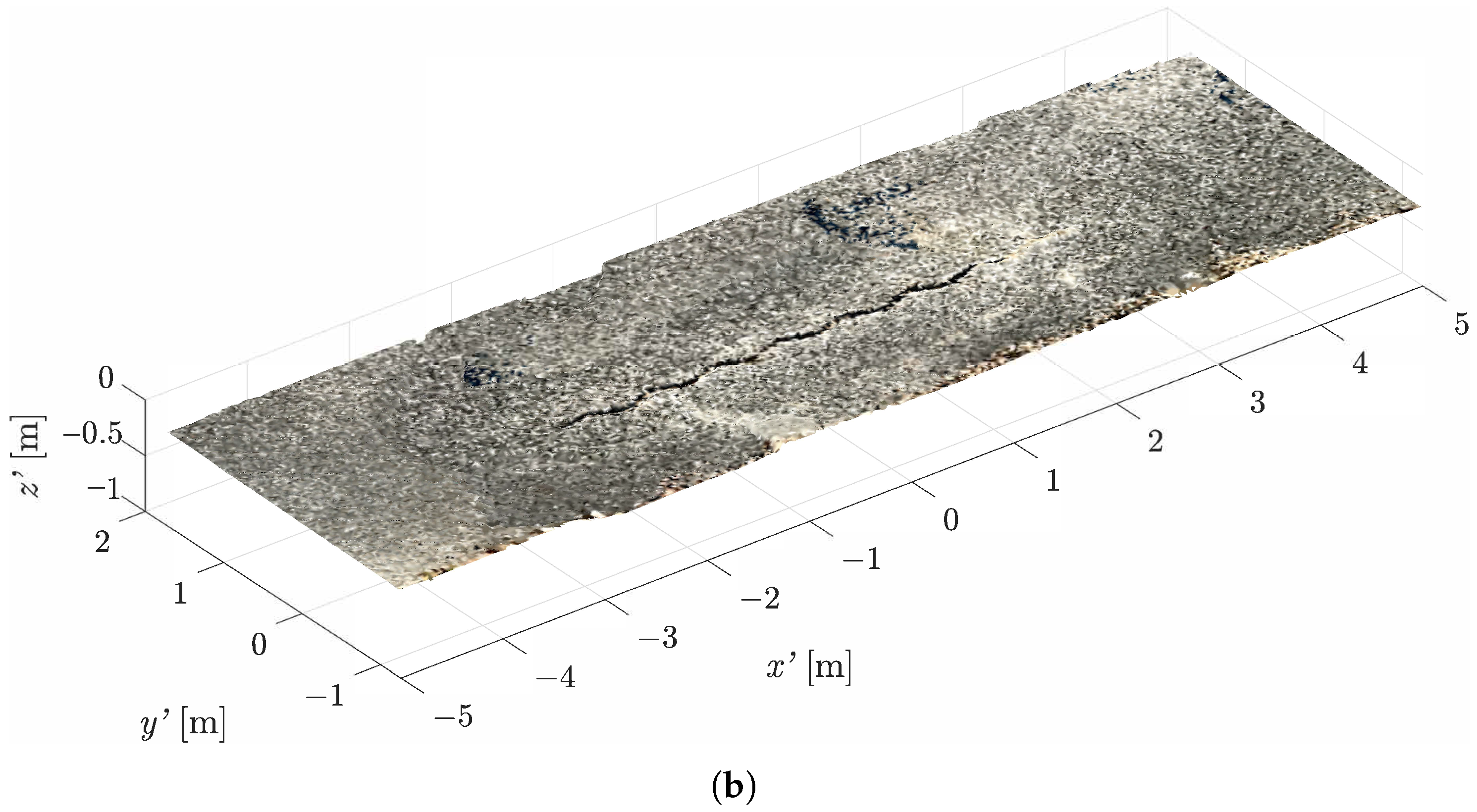
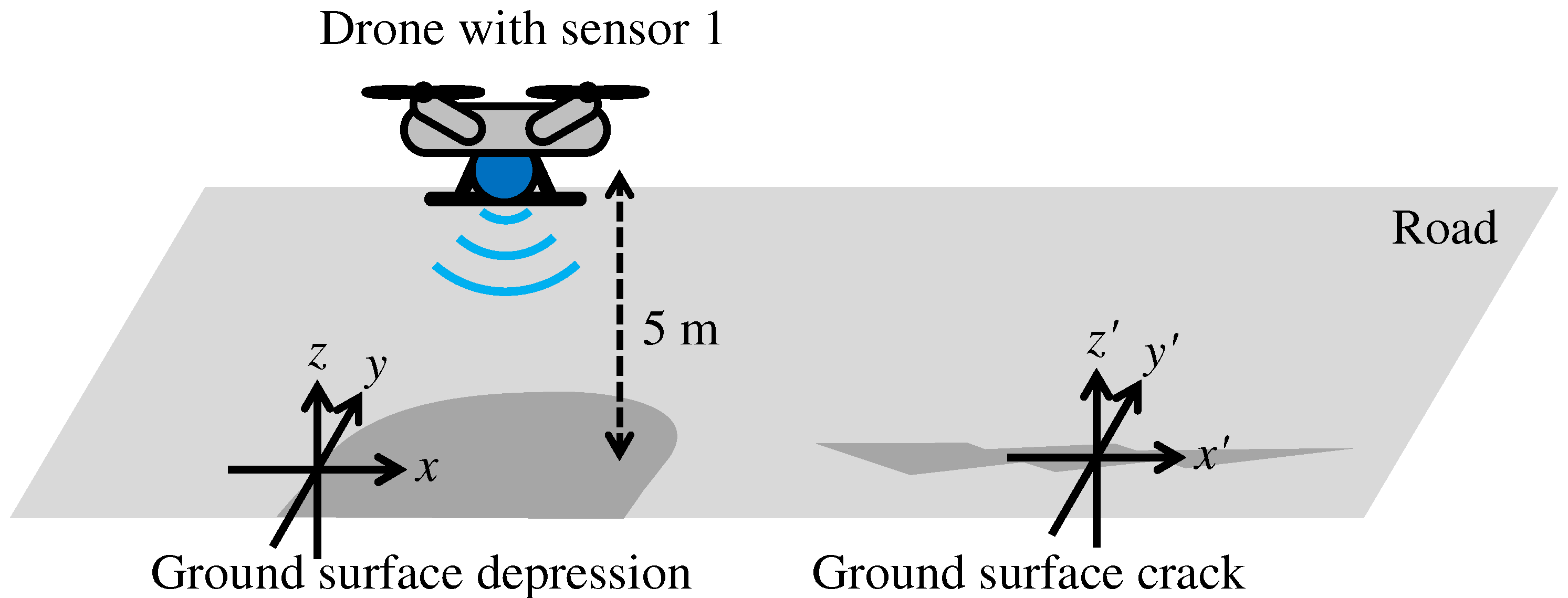
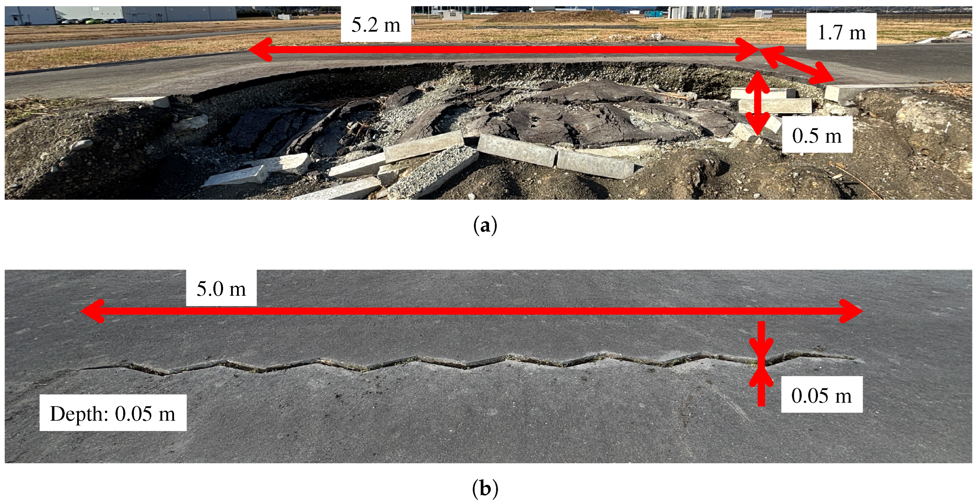
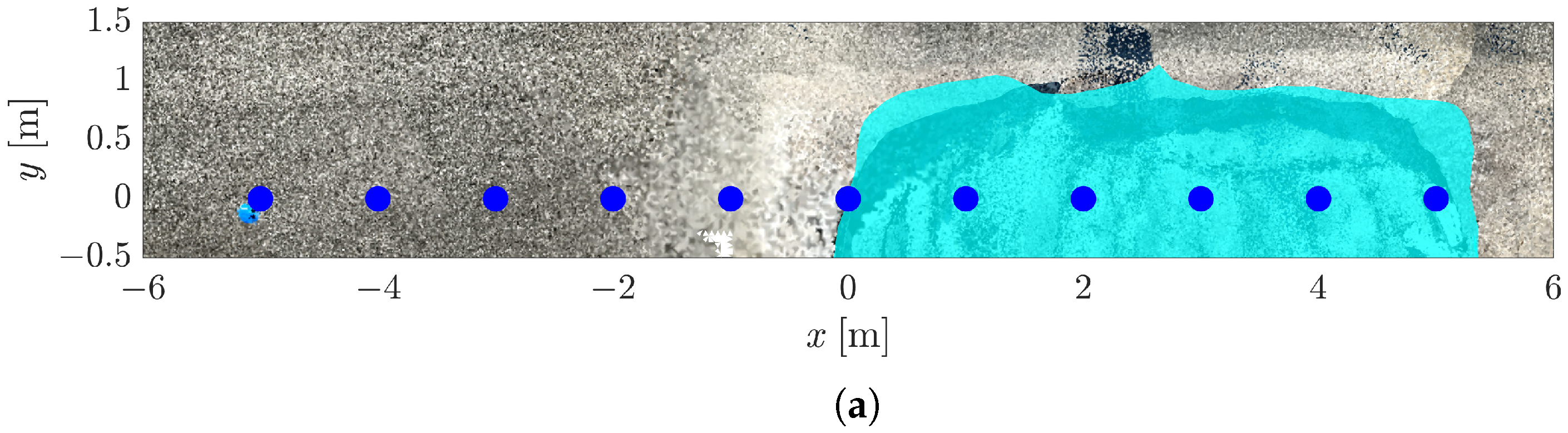
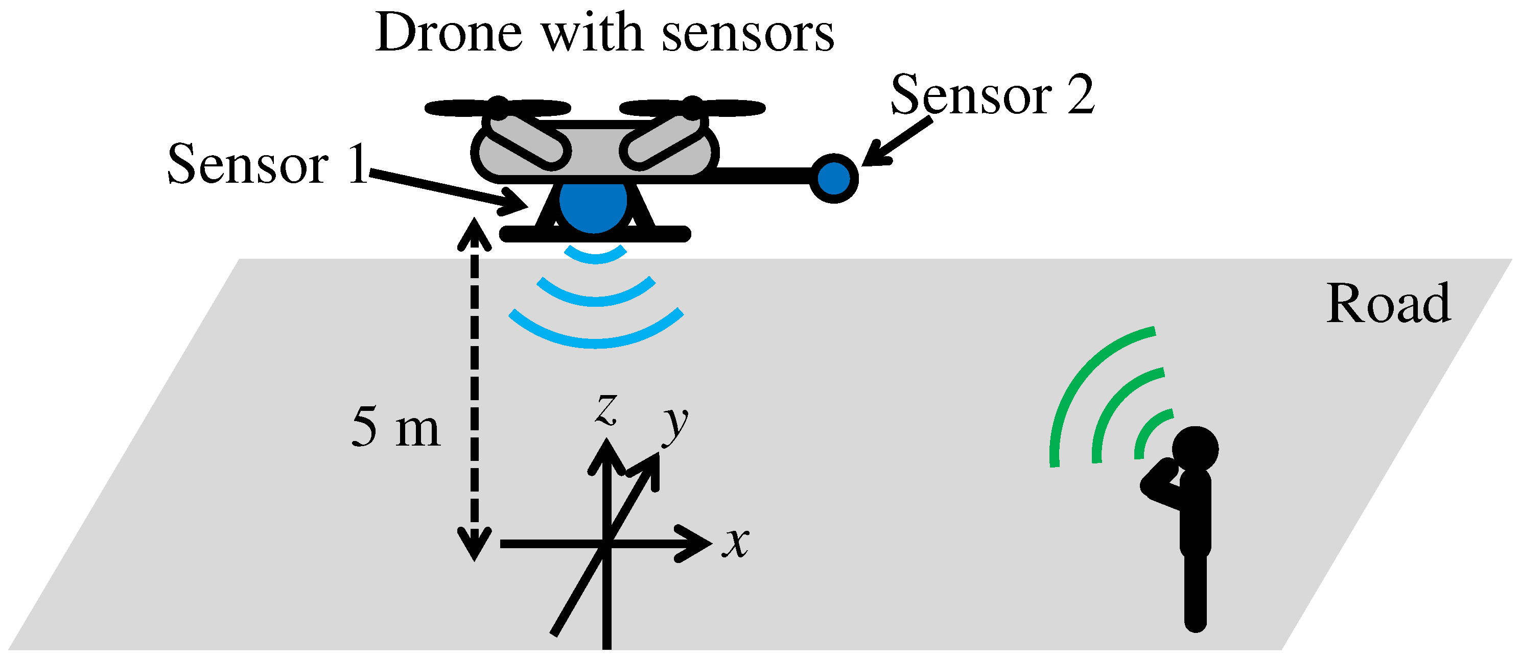
In this experiment, a ground surface depression and a ground surface crack are selected as representative examples of ground surface anomalies that may occur in disaster scenarios. The experimental configuration is shown in Figure 3. For both sensing targets, the drone hovers at an altitude of 5 m above the ground surface, and sensing is performed from above. In this study, the sensing experiments are conducted at an altitude of 5 m, which corresponds to a typical operational altitude used in our previous drone audition studies for victim search. Since the proposed sensing framework is intended to be executed simultaneously with acoustic-based victim localization, the experimental conditions are aligned with those used in victim search scenarios. In addition, this study aims to first investigate the sensing feasibility and identify practical issues under controlled experimental conditions before extending the analysis to a wider range of drone altitudes. The dimensions of the sensing targets are shown in Figure 4. The ground surface depression has a length of 5.2 m, a width of 1.7 m, and a depth of approximately 0.5 m, with a complex internal shape. The ground surface crack has a length of 5.0 m, and both its width and depth are approximately 0.05 m. In addition, as a reference for evaluation, the ground surface shapes are measured using LiDAR, as shown in Figure 5.

The experimental evaluation consists of two parts:

• Evaluation of sensing performance using different transmitted signals.
• Evaluation of the influence of sensing position on performance and sensing coverage.

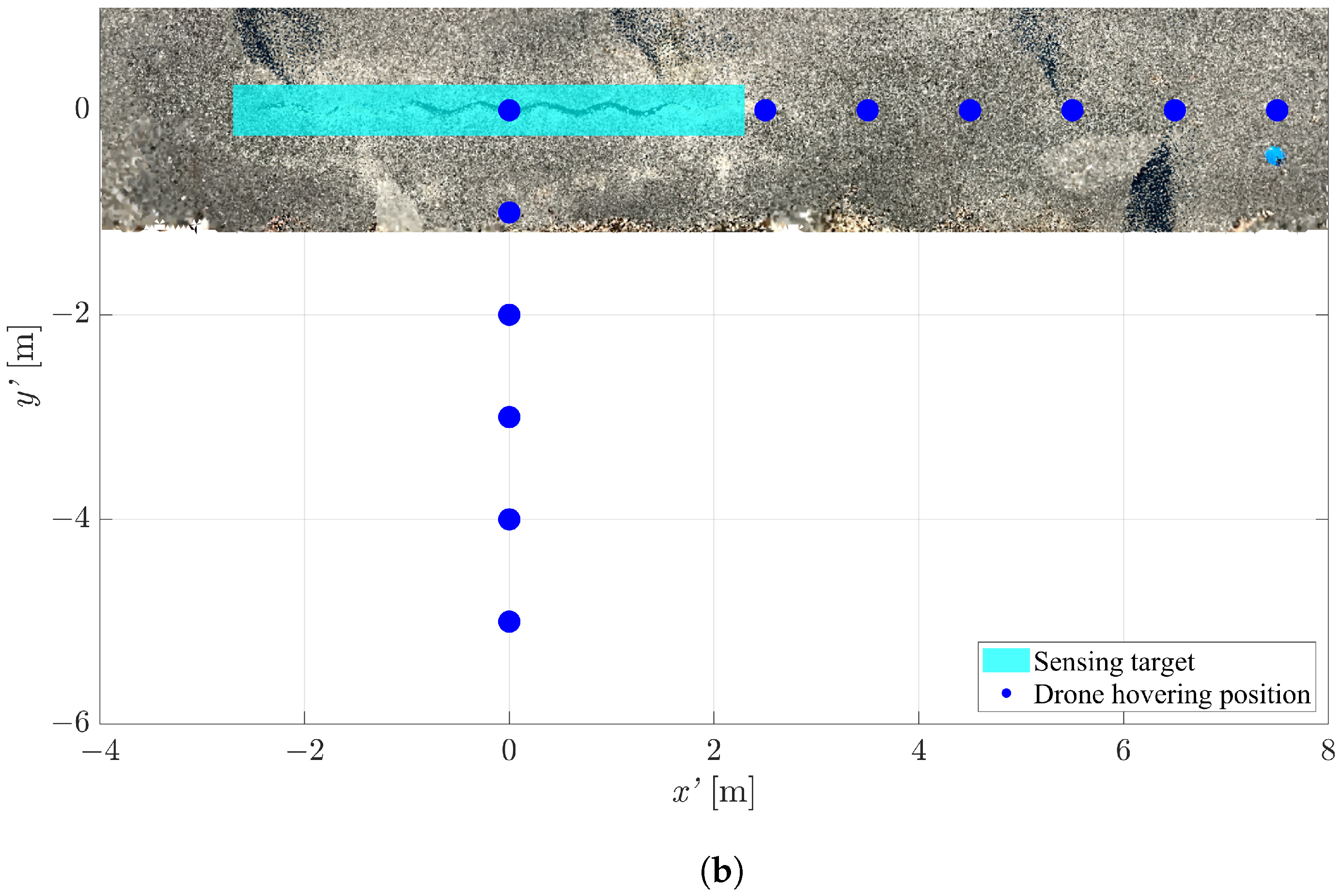
For the first evaluation, the sensing performance is investigated by varying the frequency range and duration of the transmitted chirp signals, as shown in

Table 1. Transmitted chirp signals.

	Frequency Range [kHz]	Duration [s]
Signal 1	1–5	1.0
Signal 2	1–5	0.5
Signal 3	3–5	0.5

. For the second evaluation, sensing is performed from multiple hovering positions for each sensing target, as shown in Figure 6, and the influence of sensing position and the achievable sensing coverage are evaluated. For the ground surface depression, the geometric relationship between the flat road surface and the depression remains unchanged regardless of the direction of sensor movement. Therefore, the sensing position was varied only along the x direction. In contrast, the ground surface crack has anisotropic geometric characteristics along the longitudinal ($x^{\prime }$) and transverse ($y^{\prime }$) directions. Therefore, the sensing position was varied along both directions to evaluate sensing performance with respect to these different geometrical configurations. In this evaluation, the effects of drone ego-noise and position and attitude fluctuations during hovering are also investigated.

3.1.2. Comparison of Transmitted Signals

First, the sensing performance obtained using different transmitted signals is compared. In this experiment, the effects of the chirp signal parameters, namely the frequency range and duration, on the sensing performance are evaluated in an outdoor environment. These parameters were selected because they directly influence the robustness of the sensing signal against drone ego-noise and platform motion. Narrowing the frequency range can reduce the influence of drone ego-noise, whereas a wider bandwidth improves the impulse response obtained after pulse compression. In addition, the signal duration influences the trade-off between pulse-compression gain and sensitivity to position fluctuations of the drone during transmission and reception. Therefore, multiple chirp signals with different frequency ranges and durations were tested to investigate these trade-offs.

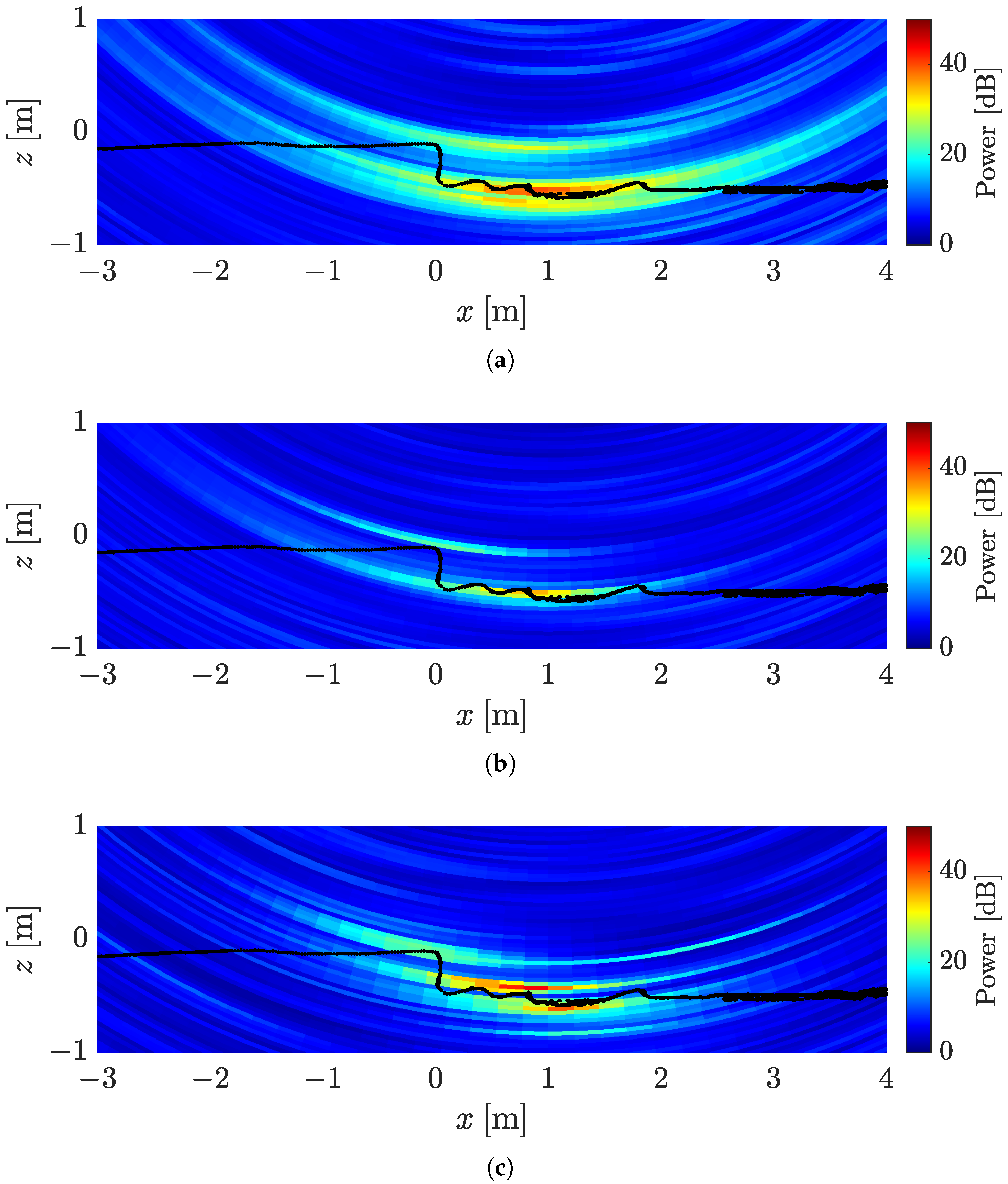
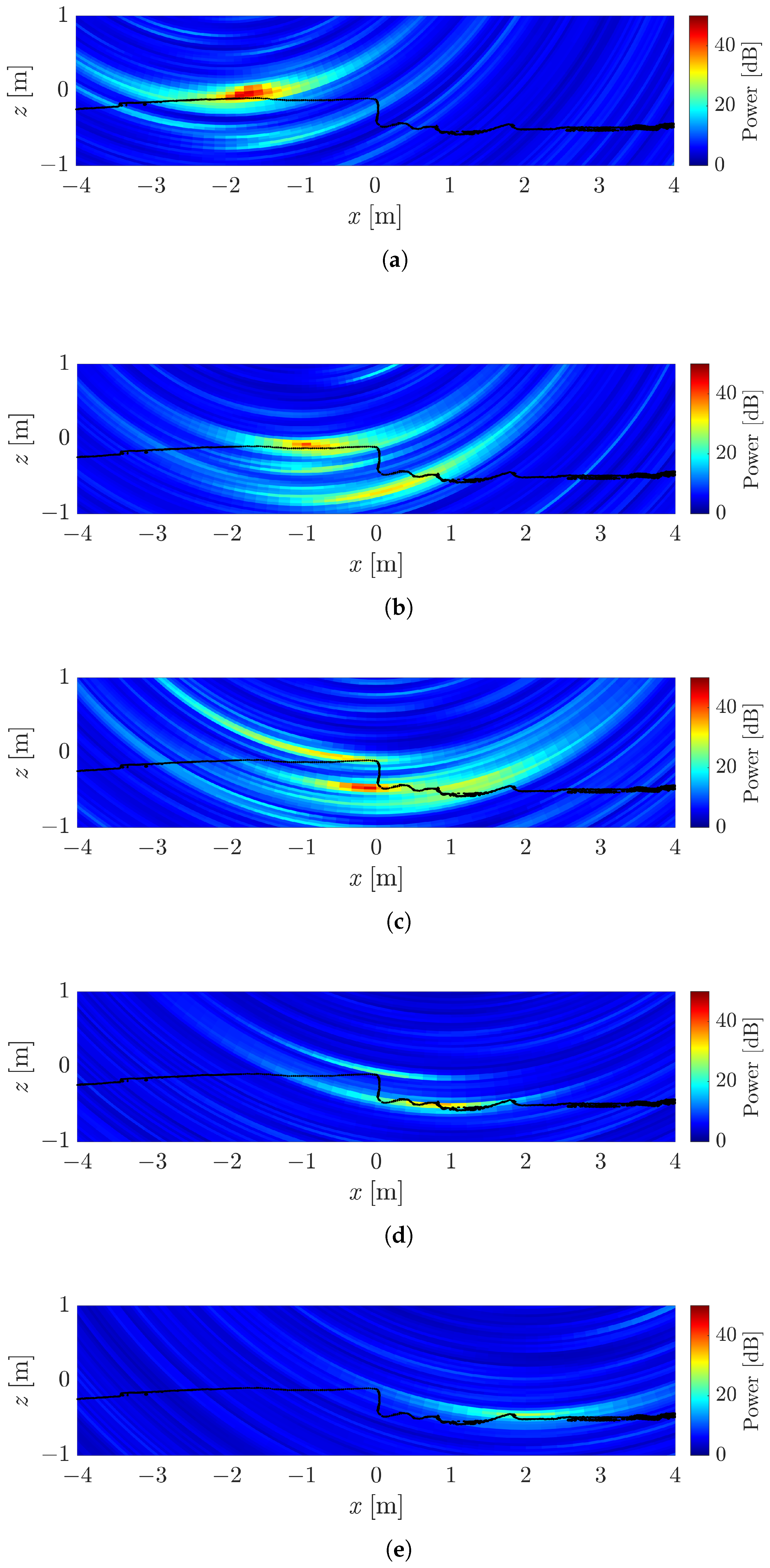
Figure 7 shows examples of two-dimensional cross-sectional sensing results for a ground surface depression, represented by the MUSIC spatial spectrum obtained using Equation (10). These results correspond to a cross section at $y=0$ m when the sensor position is $(x,y,z)=(1,0,5)$ m. The horizontal and vertical axes represent the x- and z-coordinates, respectively, and the power of the spatial spectrum is visualized using a colormap. Since the MUSIC spatial spectrum has a sharp dynamic range, it is more convenient to visualize it on a logarithmic scale rather than a linear scale. However, as shown in Equations (9) and (10), the obtained spatial spectrum values are dimensionless quantities. Therefore, a physical reference level for the logarithmic scale cannot be defined. In this paper, the reference level is set to unity, and the spatial spectrum is plotted as $20{log}_{10}\left(\overline{P^{\prime }}\right)$ [dB]. As a reference, the ground surface profile measured using LiDAR is plotted as a black line. For all transmitted signals, a high-power component can be observed directly beneath the sensor at $(x,z)=(1,-0.5)$ m. In addition, the edge of the depression located away from the sensor position at $(x,z)=(0,0)$ m can be identified for all transmitted signals.

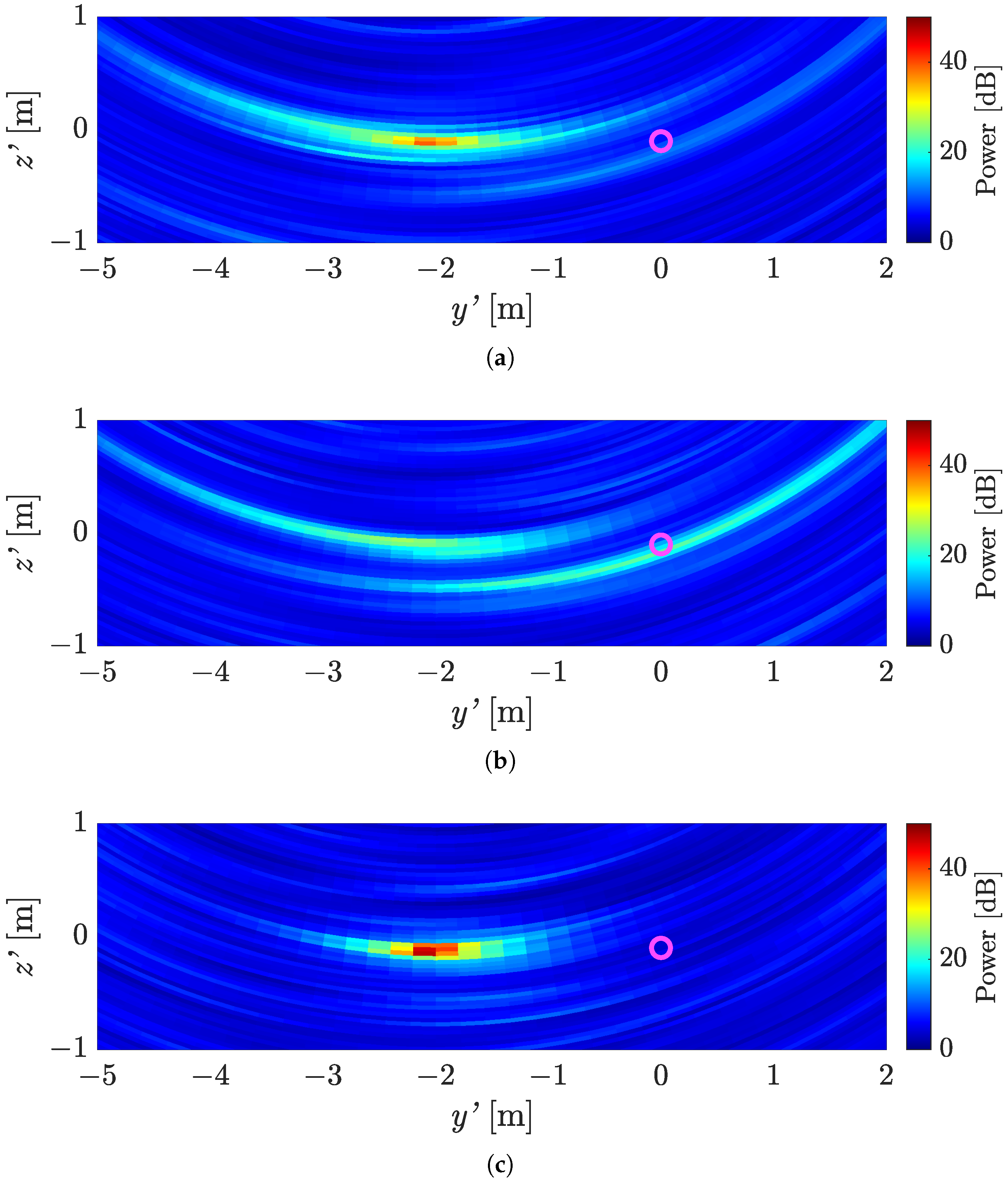
In contrast, Figure 8 shows the corresponding two-dimensional cross-sectional sensing results for a ground surface crack. These results correspond to a cross section at $x^{\prime }=0$ m when the sensor position is $(x^{\prime },y^{\prime },z^{\prime })=(0,-2,5)$ m. The horizontal and vertical axes represent the $x^{\prime }$- and $z^{\prime }$-coordinates, respectively, and the crack location is indicated by magenta circles. A high-power component can be observed directly beneath the sensor at $(y^{\prime },z^{\prime })=(-2,0)$ m. However, at the crack location $(y^{\prime },z^{\prime })=(0,0)$ m, high-power components are observed only for Signal 1 and Signal 2. This difference can be explained by the influence of the frequency bandwidth on the impulse response obtained after pulse compression. When the frequency bandwidth is narrow, the influence of drone ego-noise can be reduced. However, the impulse response becomes broader, which decreases the angular resolution of the sensing result. As a consequence, small surface anomalies such as cracks become difficult to detect when a narrow bandwidth is used. This explains why the crack location is clearly observed for Signal 1 and Signal 2 but not for Signal 3. In addition, a difference can be observed between Signal 1 and Signal 2, where Signal 2 shows higher power at the crack location. This difference is mainly related to the duration of the chirp signal. A longer chirp signal provides greater SNR improvement through pulse compression. However, it also increases the sensitivity to position and attitude fluctuations of the drone during signal transmission and reception. Such fluctuations can degrade the effective pulse-compression gain. Signal 1 has a duration of 1 s, whereas Signal 2 has a shorter duration of 0.5 s, which makes Signal 2 less sensitive to drone motion while still providing sufficient pulse-compression gain. As a result, Signal 2 provides a better balance between pulse-compression gain and robustness against drone motion in the present experimental environment. These results indicate that, for sensing targets with small surface variations such as cracks, the sensing performance strongly depends on the design of the transmitted signal, particularly the frequency bandwidth and signal duration.

To quantitatively evaluate these results,

Table 2. Power of the frequency-integrated MUSIC spatial spectrum at each target location under different transmitted signals (dB).

	Depression Edge	Crack
Signal 1	25.4	12.6
Signal 2	23.6	23.3
Signal 3	23.1	6.69

summarizes the power of the frequency-integrated MUSIC spatial spectrum at the edge of the depression and at the crack location. In addition,

Table 3. Angular and range resolutions (FWHM) at each target location under different transmitted signals.

Target	Signal	Resolution
		Angular [deg.]	Range [m]
Inside the depression	Signal 1	12.6	0.062
	Signal 2	13.8	0.072
	Signal 3	12.6	0.061
Flat road surface	Signal 1	7.3	0.064
	Signal 2	8.1	0.063
	Signal 3	2.4	0.040

presents the angular and range resolutions derived from the frequency-integrated MUSIC spatial spectrum. The resolutions are calculated based on the dominant peak corresponding to the reflection directly beneath the sensor. Specifically, for the results in Figure 7, the values are obtained from the reflection inside the depression, whereas for Figure 8, they are obtained from the reflection from the flat road surface. The values shown in the tables are averages over ten trials. At the edge of the depression, powers exceeding 20 dB are observed for all transmitted signals, whereas at the crack location, only Signal 2 achieves a power exceeding 20 dB. Regarding angular resolution, larger values are observed inside the depression for all signals due to the complex geometry and the mixture of multiple reflections. In contrast, on the flat road surface, Signal 3 achieves the smallest angular resolution, while Signals 1 and 2 show comparable performance. The range resolution is approximately 0.06 m under all conditions. These observations are physically consistent with the signal modeling of chirp signals, considering the effects of bandwidth, duration, and motion-induced phase errors in drone-mounted sensing. With respect to the frequency range, narrowing the bandwidth and shifting it toward higher frequencies improves angular resolution. However, this reduces the pulse-compression gain, making it difficult to detect small surface anomalies such as cracks. In contrast, a wider bandwidth provides higher pulse-compression gain, enabling the detection of small anomalies, although at the cost of degraded angular resolution. With respect to signal duration, a longer signal provides greater pulse-compression gain, but it also increases sensitivity to drone position and attitude fluctuations during transmission and reception. In drone-mounted sensing scenarios, shortening the duration helps suppress the influence of such fluctuations.

Based on these results, in drone-based acoustic sensing, increasing the bandwidth while shortening the signal duration improves detection performance. On the other hand, improving angular resolution requires a narrower and higher-frequency band, which introduces a trade-off with pulse-compression gain and spatial directivity. In particular, higher-frequency components lead to sharper directivity, which narrows the effective sensing area and limits spatial coverage. Under the experimental conditions of this study, Signal 2 is confirmed to be suitable for sensing both ground surface depressions and cracks. In the following experiments, only Signal 2 is used as the transmitted signal.

3.1.3. Effect of Sensing Position

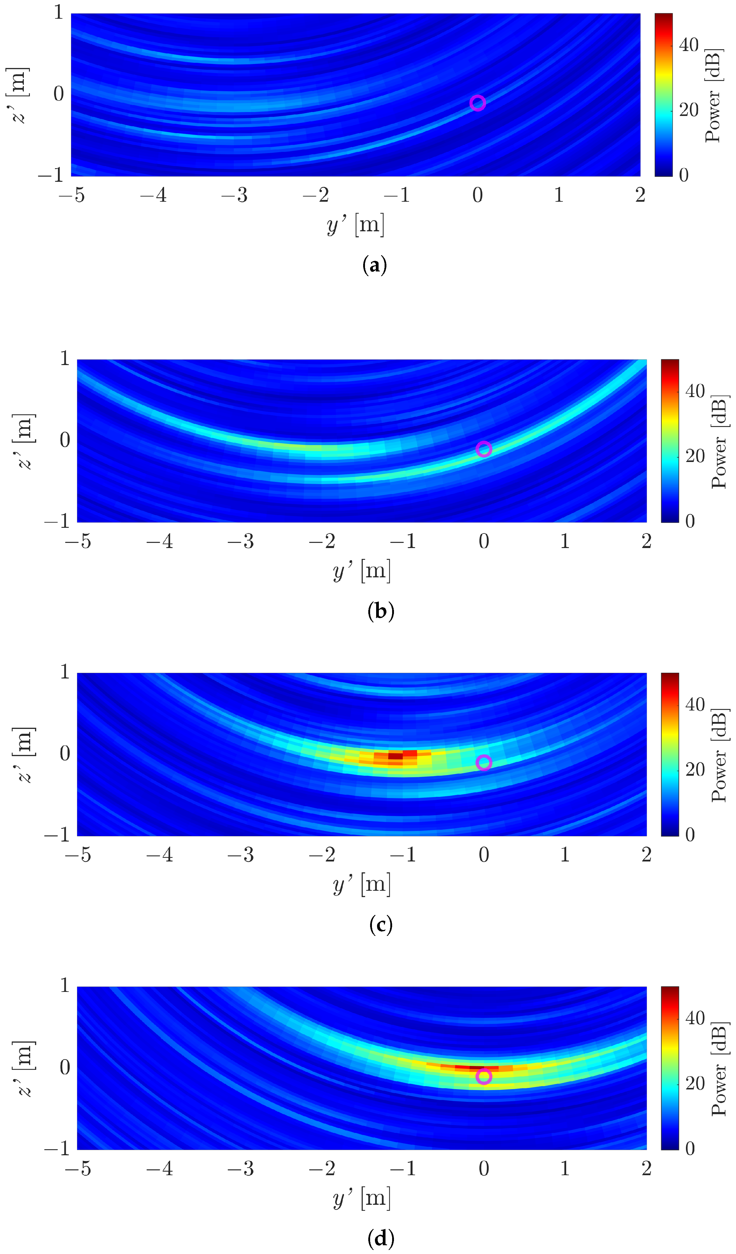
Next, the influence of sensing position on active acoustic sensing performance is evaluated. As shown in Figure 7 and Figure 8, reflections directly beneath the sensor can be readily observed. Therefore, it is important to investigate how sensing performance changes when the drone hovers away from the target location and to determine the effective horizontal sensing range. The sensing positions are shown in Figure 6. For the ground surface depression, the region $-5\le x\le 0$ m corresponds to a flat road surface, $x=0$ m corresponds to the depression edge, and $0\le x\le 5$ m corresponds to the inside of the depression. The drone hovering position was varied along the x-axis from $x=-5$ to 5 m at 1 m intervals. For the ground surface crack located at $-2.5\le x^{\prime }\le 2.5$ m and $y^{\prime }=0$ m, sensing was performed by varying the drone position in two directions: (1) along the $x^{\prime }$ direction from $x^{\prime }=2.5$ to $7.5$ m at 1 m intervals, moving away from the longitudinal end of the crack, and (2) along the $y^{\prime }$ direction from $y^{\prime }=0$ to $-5$ m at 1 m intervals, moving away in the transverse direction. In all experiments, the drone altitude was 5 m.

Figure 9 shows examples of two-dimensional cross-sectional sensing results for the depression at different drone positions. The results correspond to a two-dimensional cross section at $y=0$ m. The ground surface profile measured using LiDAR is also plotted as a black line for reference. When the drone hovers at $x=-2$ m, both the flat road surface directly beneath the sensor and the depression edge can be observed. As the drone approaches the edge ($x\to 0$ m), the power of the edge component increases, and reflections from inside the depression become visible. However, when the drone moves further inside the depression ($x>0$ m), the flat road surface component disappears. At $x=2$ m, the edge component also becomes difficult to observe. These results indicate that sensing performance strongly depends on the horizontal offset between the sensor and the target location.

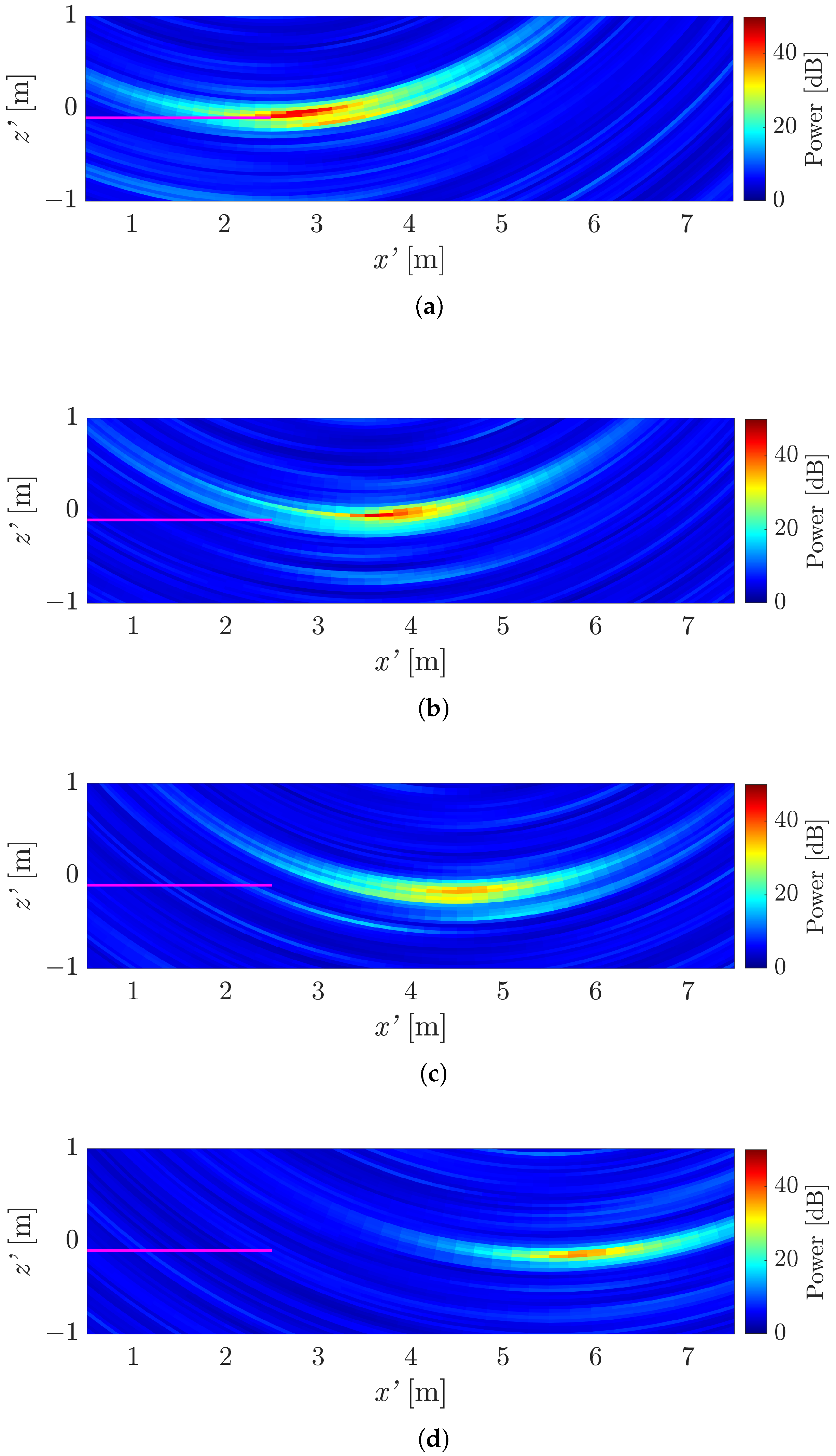
Figure 10 shows examples of two-dimensional sensing results for the crack when the drone position is varied along the $x^{\prime }$ direction. The results correspond to a two-dimensional cross section at $y^{\prime }=0$ m, and the crack location is indicated by magenta lines. Figure 11 shows the corresponding sensing results when the drone position is varied along the $y^{\prime }$ direction. The results correspond to a two-dimensional cross section at $x^{\prime }=0$ m, and the crack location is indicated by magenta circles. As the drone moves away from the crack along the $x^{\prime }$ and $y^{\prime }$ directions, the component corresponding to the crack gradually decreases in power, and becomes difficult to observe when the horizontal offset increases. When the drone hovers near the crack (e.g., $x^{\prime }=2.5$–$3.5$ m or $y^{\prime }=-1$–0 m), two components can be observed in the $z^{\prime }$ direction: reflections from the flat road surface and reflections from inside the crack. This indicates that even for a crack with a depth of approximately 0.05 m, height differences inside and outside the crack can be detected under favorable positioning conditions. However, the separation of these two components is still limited in the current results, and improving the separation between reflections from the road surface and those from inside the crack remains an important topic for future work.

To quantitatively evaluate the sensing coverage, the detection success rate was calculated for each sensing position. Detection was defined as successful when a component with power exceeding 15 dB was observed within 0.15 m of the target location. These thresholds were selected empirically to ensure robust discrimination between target reflections and background components. The success rate was computed over 10 trials. To further investigate the influence of drone ego-noise and position and attitude fluctuations, detection success rates were also calculated under three conditions:

• Signals recorded using a fixed sensor at the hovering position (no ego-noise or fluctuations),
• Signals obtained by adding separately recorded drone ego-noise to the fixed-sensor recordings (ego-noise only),
• Signals recorded using the drone-mounted sensor (ego-noise and fluctuations).

This comparison enables the separate evaluation of the influence of ego-noise alone and the combined influence of ego-noise and fluctuations.

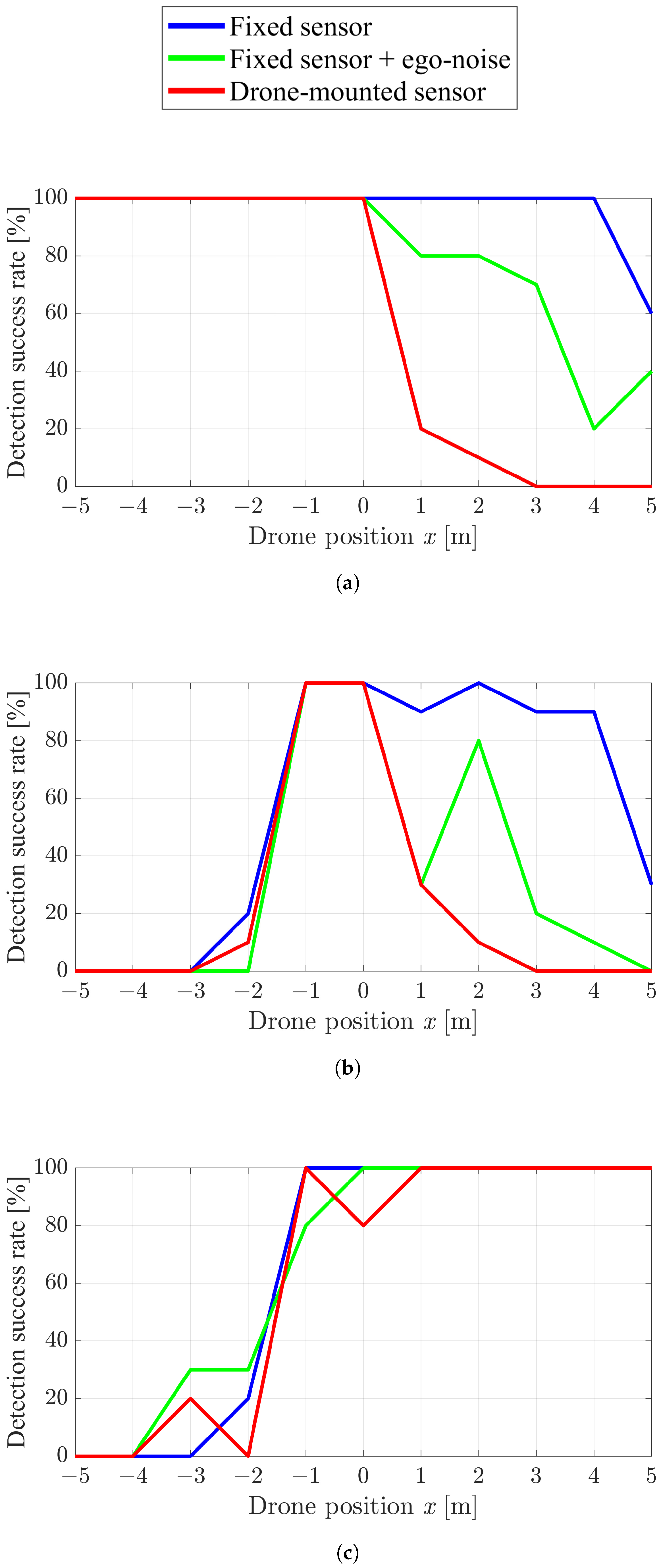
Figure 12 shows the detection success rates for the depression. In the figures, the blue line represents the results obtained using the fixed sensor, the green line represents the results obtained by adding separately recorded drone ego-noise to the fixed-sensor recordings, and the red line represents the results obtained using the drone-mounted sensor. For the flat road surface (Figure 12a), the success rate decreases as the drone moves away from the target. The addition of ego-noise and fluctuations further degrades performance. This can be explained by the specular reflection characteristics of flat surfaces: when the sensing signal is incident at oblique angles, the reflected wave does not efficiently return to the sensor, making the system more sensitive to SNR degradation and fluctuations. For the depression edge (Figure 12b), high detection success rates are maintained near $-1\le x\le 0$ m under all sensing conditions. However, the success rate drops significantly when $x\le -2$ m. On the other hand, for $x\ge 0$ m, the detection success rate is high when neither ego-noise nor fluctuations are present, however, it decreases similarly in the cases with ego-noise only and with both ego-noise and fluctuations. This indicates that the performance degradation in this region is primarily caused by ego-noise, while the additional influence of fluctuations is relatively limited. This is likely because edges scatter acoustic waves over a wider range of angles compared to flat surfaces, making detection less sensitive to incident angle variations. For the inside of the depression (Figure 12c), high success rates are observed near the edge region, but performance decreases rapidly when the drone moves further away. This is attributed to geometric constraints: as the horizontal offset increases, acoustic waves are less likely to propagate effectively into the inside region.

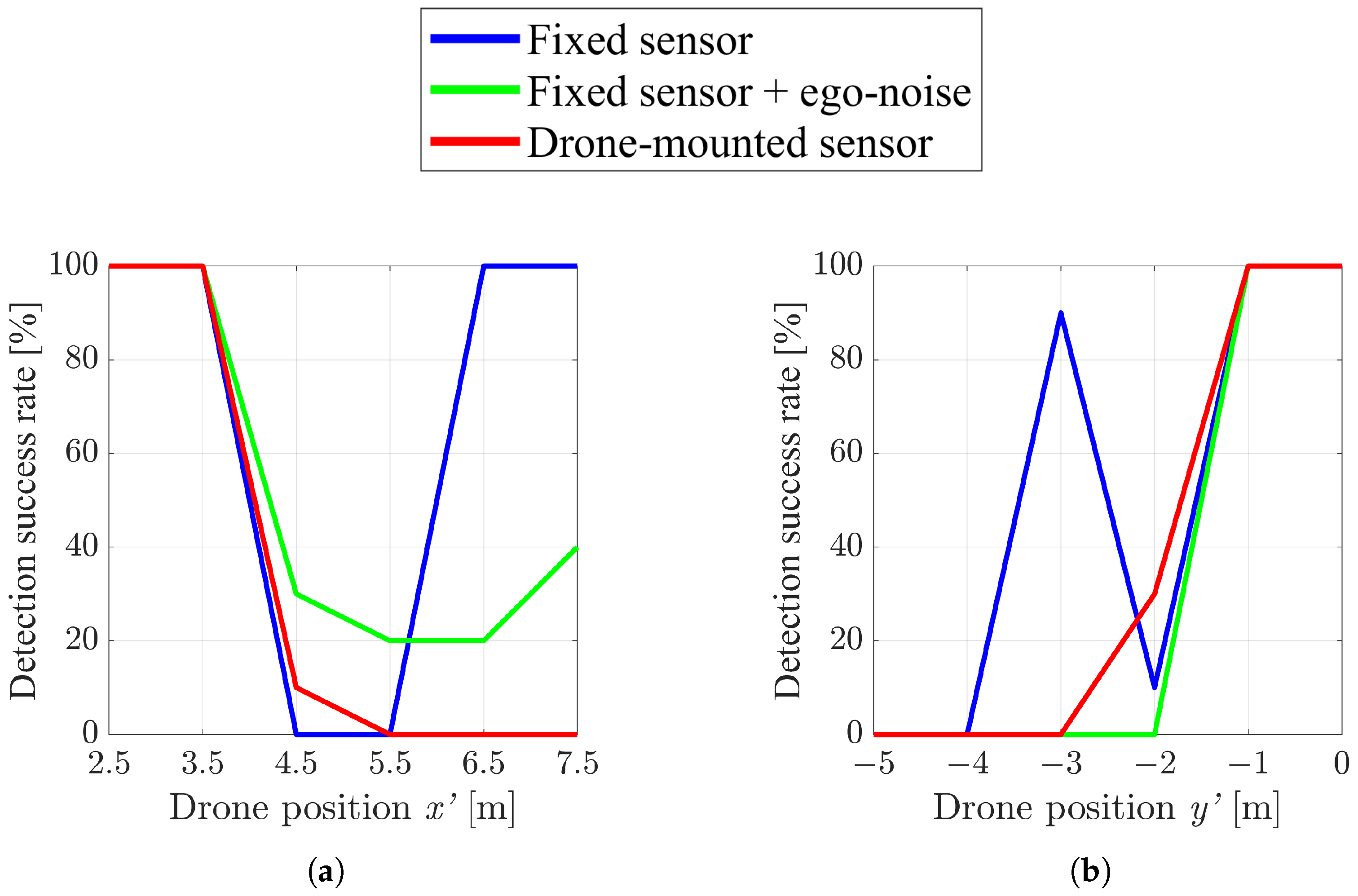
Figure 13 shows the detection success rates for the crack. For both variations along the $x^{\prime }$ and $y^{\prime }$ directions, high detection success rates are maintained within approximately 1 m from the crack. Beyond 2 m, the success rate drops significantly. The effective sensing range for the crack is therefore comparable to that of the depression, and no substantial anisotropy is observed between the longitudinal and transverse directions.

Although the overall tendency is consistent with the expected sensing geometry, some irregular variations can be observed in the detection success rates in the results obtained using the fixed sensor. These variations are likely caused by complex acoustic propagation phenomena in the real outdoor environment, such as multipath reflections from surrounding structures and surface roughness of the road surface. Because the experiments were conducted under real operating conditions, such effects are difficult to control completely and may lead to unexpected variations in the results, particularly in the fixed-sensor results where drone ego-noise is absent and the SNR is relatively high, making the influence of multipath reflections more apparent. Nevertheless, these observations provide useful insights into the practical limitations of the proposed sensing framework. A more detailed investigation of these phenomena, including controlled numerical simulations and parametric analyses, will be conducted in future work to better understand the underlying mechanisms and to improve sensing robustness.

The results clarify the current sensing coverage limitation of the proposed framework under the experimental altitude of 5 m used in this study. From a geometric viewpoint, increasing the drone altitude would enlarge the ground coverage area observable from a single sensing position. However, as the altitude increases, the propagation distance between the drone and the ground surface also becomes larger, which reduces the SNR of the reflected signals due to geometric spreading loss and atmospheric attenuation. In addition, the spatial resolution of the sensing system may degrade as the sensing distance increases. Therefore, extending the sensing range while maintaining sufficient sensing performance at higher drone altitudes remains an important challenge.

To address these limitations, further investigations are required regarding sensor configuration, sensing signal design, and signal processing methods that are robust against ego-noise and fluctuations during drone operation. In addition, future work should consider sensing scenarios in which the drone moves continuously while performing sensing. In such cases, additional factors such as variations in ego-noise, aerodynamic noise, and Doppler effects caused by drone motion may influence sensing performance and should be investigated.

3.2. Simultaneous Acoustic Sensing and Sound Source Localization

3.2.1. Experimental Setup

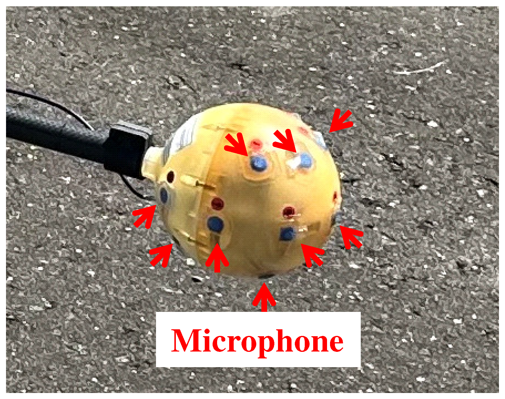
In Section 3.1, the performance of active acoustic sensing alone was evaluated. In this subsection, the feasibility and performance of the simultaneous execution of active acoustic sensing and SSL are evaluated using signals recorded in a real outdoor environment as well as signals generated by numerical simulations. It should be noted that the objective of this experiment is not to perform a detailed performance comparison between different sensor configurations. Rather, the goal is to verify the feasibility of performing active acoustic sensing and SSL simultaneously using a compact sensing system. A detailed investigation of the influence of individual design factors, such as sensor configuration, array geometry, and signal processing parameters, remains an important topic for future work. In addition to Sensor 1, a microphone array (Sensor 2) that has been used in previous drone audition studies for victim search [37] is employed as a reference. Sensor 2 is shown in Figure 14. Sensor 2 consists of 16 microphones arranged spherically with a diameter of 110 mm. As shown in Figure 2b, Sensor 2 is mounted at the end of a pipe attached to the drone.

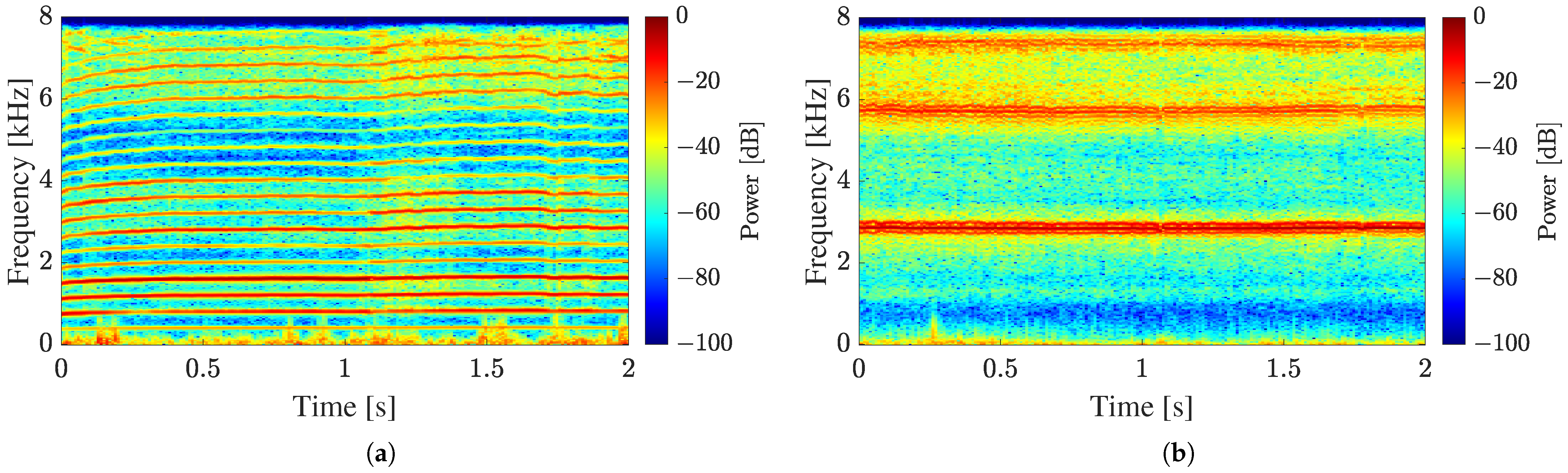
The experimental configuration is shown in Figure 15. The active acoustic sensing in this experiment targets a flat road surface. Similar to the experiments in Section 3.1, the drone hovers at an altitude of 5 m while sensing signals are transmitted from Sensor 1 and reflected signals from the ground surface are recorded. Signal 2 is used as the sensing signal. For comparison, acoustic signals are simultaneously recorded using Sensor 2 with a sampling frequency of 16 kHz and a quantization resolution of 24 bits. Furthermore, localization target sounds arriving from arbitrary directions are generated by numerical simulation and added to the signals recorded in the real environment. This evaluation method, in which simulated localization target sounds are added to noise signals recorded in real environments, has been employed in our previous studies on drone audition [16,17,18]. In those studies, the validity of this approach was confirmed by comparing localization results obtained using simulated target sounds with those obtained from real sound source experiments. By adopting the same evaluation framework in this study, the results can be directly compared with our previous findings while maintaining consistency in the evaluation methodology. By analyzing these combined signals, the feasibility of simultaneous active acoustic sensing and SSL is investigated. Figure 16 shows spectrograms of the localization target sounds used in the experiment. In this experiment, human voice and whistle sounds are used as localization targets. For the voice signal, the recorded sample does not consist of spoken sentences but rather prolonged calls for help that would realistically occur in disaster situations (e.g., sustained calls such as “Hey!” or “Help!”).

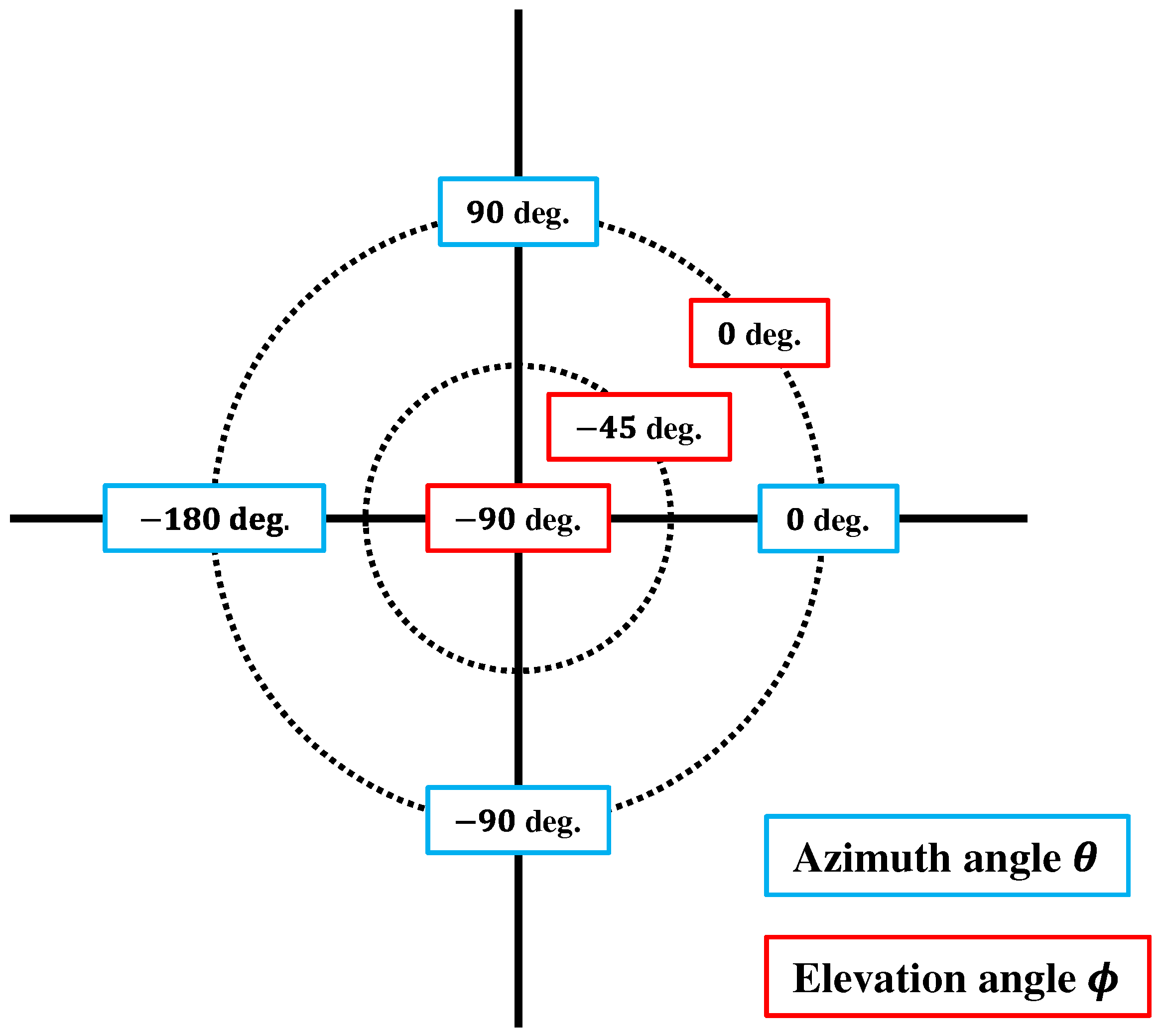
For SSL, a coordinate system is defined as shown in Figure 17, and the MUSIC spatial spectrum $\overline{P}$ in Equation (4) is plotted. The circumferential and radial directions represent the azimuth $\theta$ and elevation $\varphi$ angles, respectively. The azimuth angle is defined such that $\theta =0$ deg. corresponds to the forward direction of the drone and $\theta =-180$ deg. corresponds to the backward direction. The elevation angle is defined such that $\varphi =0$ deg. corresponds to the horizontal direction and $\varphi =-90$ deg. corresponds to the vertically downward direction of the drone.

The experimental evaluation consists of three parts:

• Evaluation of the effect of microphone array configuration on SSL performance,
• Evaluation of the influence of active acoustic sensing on SSL performance,
• Evaluation of the influence of localization target sounds on acoustic sensing performance.

For the first evaluation, the SSL performance of Sensor 1 is evaluated by comparing it with that of Sensor 2, which has been used in previous victim search studies. For the second evaluation, SSL is analyzed using signals obtained by adding numerically simulated localization target sounds to the sensing signals recorded in the real environment, and the influence of sensing signals during active acoustic sensing on localization performance is evaluated. In the first and second evaluations, SSL is performed using both Sensor 1 and Sensor 2. For the third evaluation, acoustic sensing is analyzed using the same signals, and the influence of localization target sounds on sensing performance is evaluated.

3.2.2. Effect of Microphone Array Configuration on Sound Source Localization

First, the effect of microphone array configuration on SSL performance is evaluated. In this evaluation, signals are constructed by combining drone ego-noise recorded during flight using Sensor 1 and Sensor 2 with numerically simulated localization target sounds, and are analyzed using the SSL method described in Section 2.1. These signals are recorded without transmitting sensing signals. In previous victim search studies, Sensor 2 has been installed at a position away from the drone rotors in order to reduce the influence of drone ego-noise. In contrast, Sensor 1 used in this study is mounted on the lower part of the drone body and is therefore located closer to the ego-noise sources than Sensor 2. This evaluation investigates how such differences in sensor placement affect SSL performance.

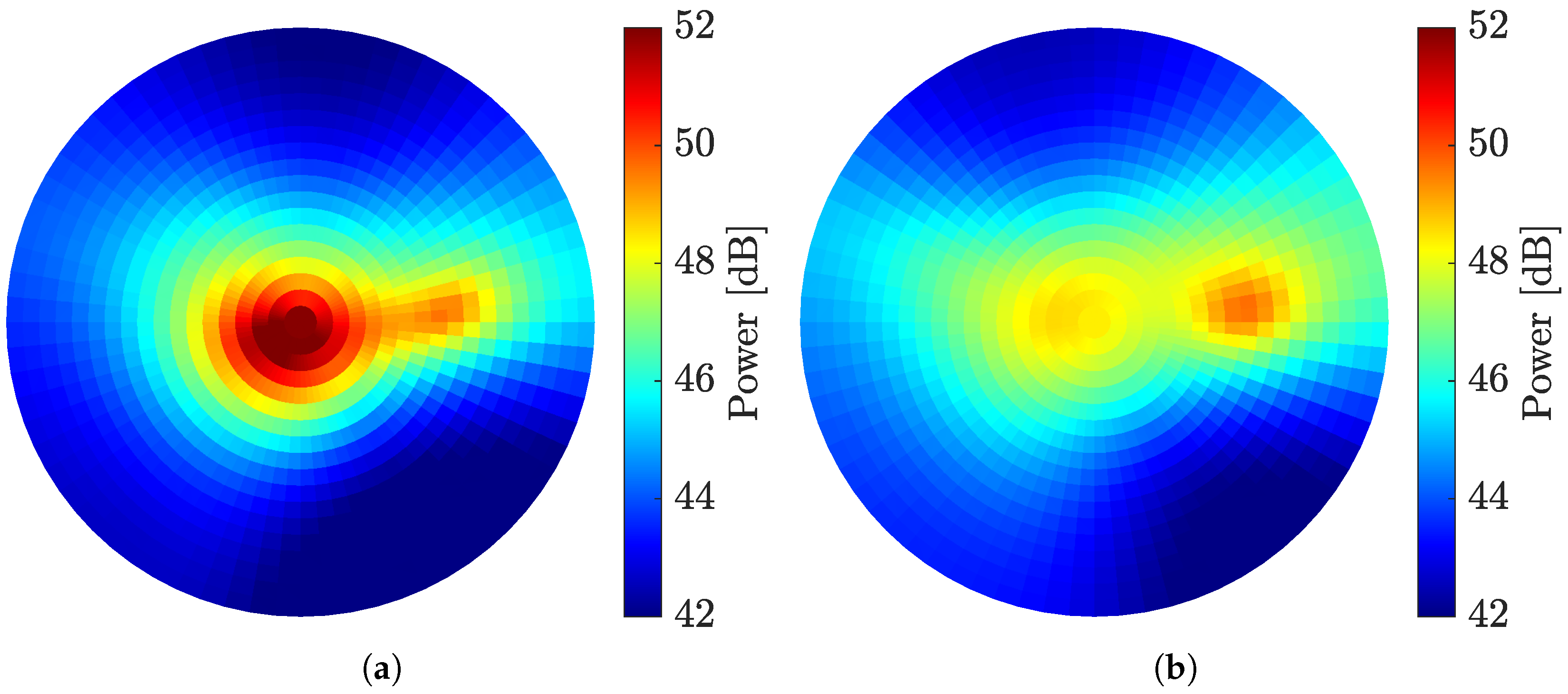
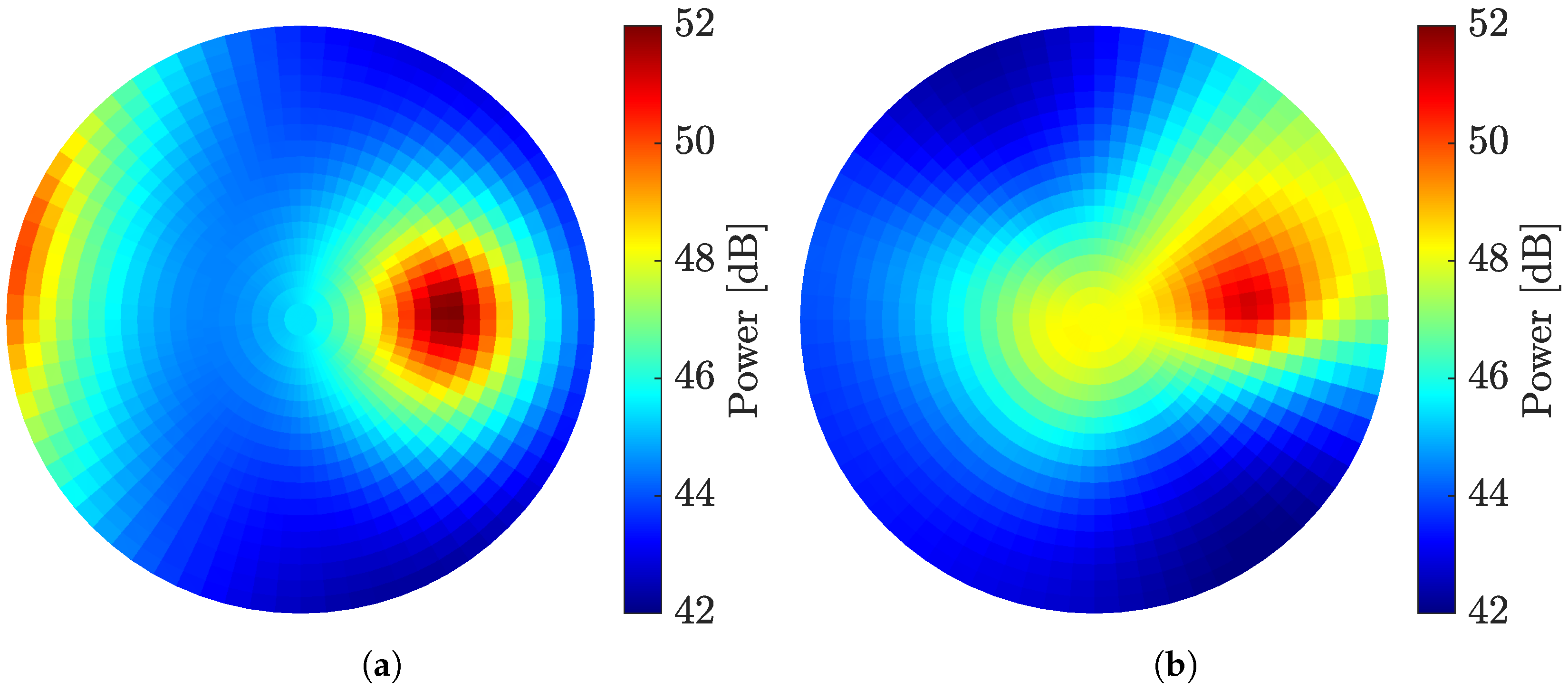
Figure 18 shows the MUSIC spatial spectrum $\overline{P}$ obtained using Equation when the localization target sound is a voice signal. Figure 18a presents the results obtained using Sensor 2, while Figure 18b presents those obtained using Sensor 1. The spatial spectrum $\overline{P}$ is plotted according to the coordinate system shown in Figure 17, where the power of sounds arriving from each direction is visualized using a colormap. Note that the spatial spectrum is visualized in dB using the same definition described in Section 3.1.2. Since the MUSIC spatial spectrum is a dimensionless quantity as shown in Equations (3) and (4), the logarithmic representation is defined with a reference value of unity, and the spectrum is plotted as $20{log}_{10}\left(\overline{P}\right)$ [dB]. The DOA of the localization target sound is set to $(\theta ,\varphi )=(0,-45)$ deg., and the signal is added such that the SNR of the localization target sound relative to drone ego-noise is $-10$ dB. For simplicity in the comparison, the SNR used in this evaluation is defined with respect to Sensor 2. The amplitude of the recorded noise signals obtained from each sensor is kept unchanged, while the amplitude of the simulated target sound is adjusted to generate signals with a specified SNR. Specifically, the target sound level is determined so that the resulting SNR corresponds to the specified value when the target sound is added to the noise signal recorded by Sensor 2. The same target sound is then added to the noise signal recorded by Sensor 1. Therefore, if Sensor 1 has higher robustness to noise than Sensor 2, the effective SNR in the Sensor 1 signals becomes higher than the specified SNR. This approach enables the evaluation of SSL performance while implicitly reflecting the noise robustness of each sensor configuration. For both sensors, a high-power component can be observed near $(\theta ,\varphi )=(0,-45)$ deg., corresponding to the localization target sound. In the result obtained using Sensor 2, an additional high-power component is observed near $\theta =-180$ deg. This component corresponds to drone ego-noise, which has been shown in previous studies to degrade SSL performance. In contrast, in the result obtained using Sensor 1, a component considered to be caused by ego-noise is observed near $\varphi =-90$ deg., however, its power is lower than that observed in Figure 18a. This difference can be attributed to the sensor placement. In the case of Sensor 2, there is no physical shielding between the ego-noise sources and the sensor, and therefore the ego-noise is received with relatively little attenuation despite the larger distance. In contrast, for Sensor 1, the drone body acts as a physical shield between the ego-noise sources and the sensor, resulting in attenuation of the ego-noise before it reaches the sensor.

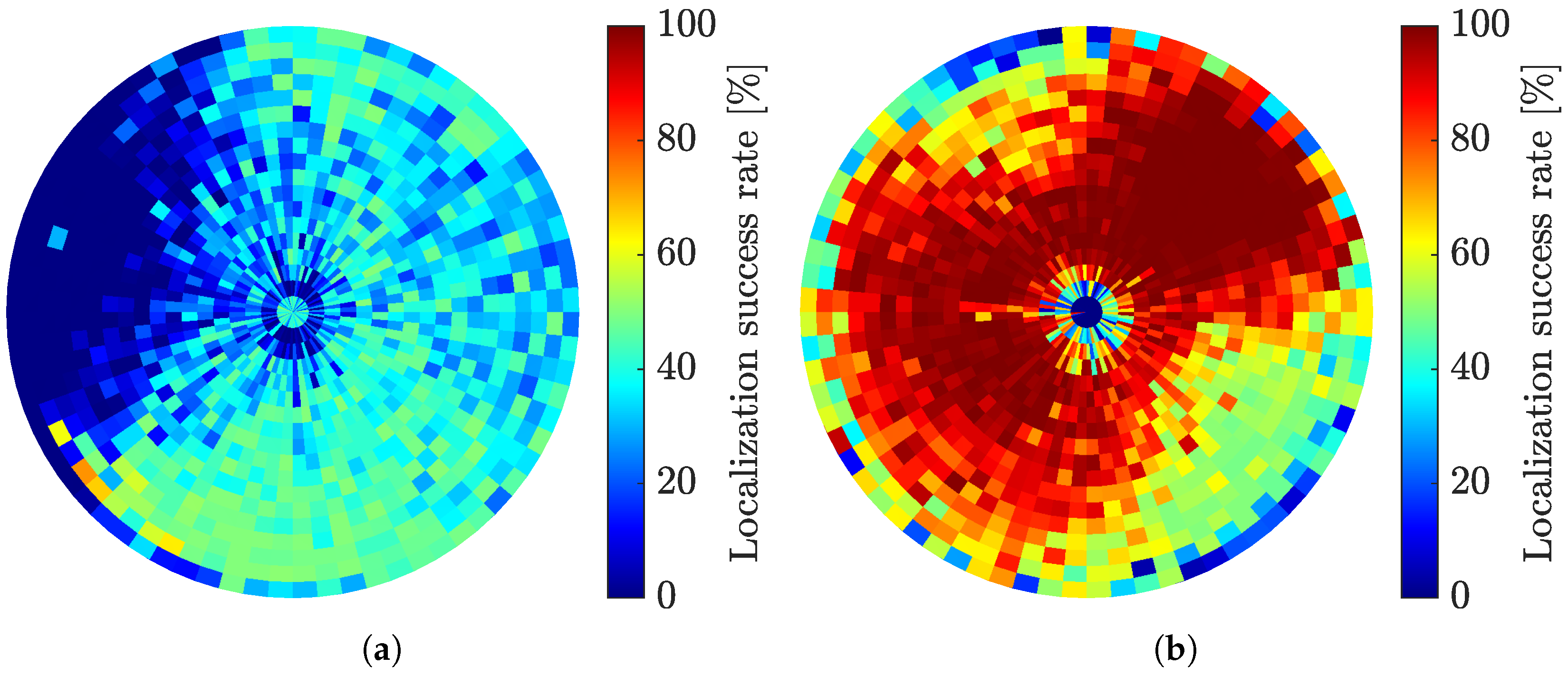
To quantitatively evaluate localization performance, the DOA of the localization target sound is varied over the range $-180\le \theta \le 180$ deg. and $-90\le \varphi \le 0$ deg. For each target direction, 100 trials are conducted with an SNR of $-10$ dB. Localization is defined as successful when the estimated direction ${\psi }_{target}$ obtained using Equation (5) matches the preset target direction. The localization success rate for each direction is calculated using the results obtained with both voice and whistle target sounds. Figure 19 shows the resulting localization success rates. Figure 19a presents the results obtained using Sensor 2, while Figure 19b presents those obtained using Sensor 1. Similar to the MUSIC spatial spectra, the success rates are plotted according to the coordinate system shown in Figure 17, and visualized using a colormap. When Sensor 2 is used, the localization success rate is close to 0% near $\theta =-180$ deg., where strong ego-noise components are present. In addition, the success rate in other directions is reduced to approximately 50% due to the influence of ego-noise. In contrast, when Sensor 1 is used, the ego-noise components have lower power, as shown in Figure 18b, and thus have little impact on localization performance. As a result, localization success rates exceeding 90% are achieved for almost all directions.

Although MUSIC-based SSL methods that suppress the influence of ego-noise have been proposed [38,39,40,41], the results demonstrate that placing the sensor on the lower part of the drone, as in Sensor 1, can significantly improve localization performance without requiring such computationally expensive methods. These results demonstrate that the active acoustic sensing sensor is also effective for SSL.

3.2.3. Effect of Acoustic Sensing on Sound Source Localization

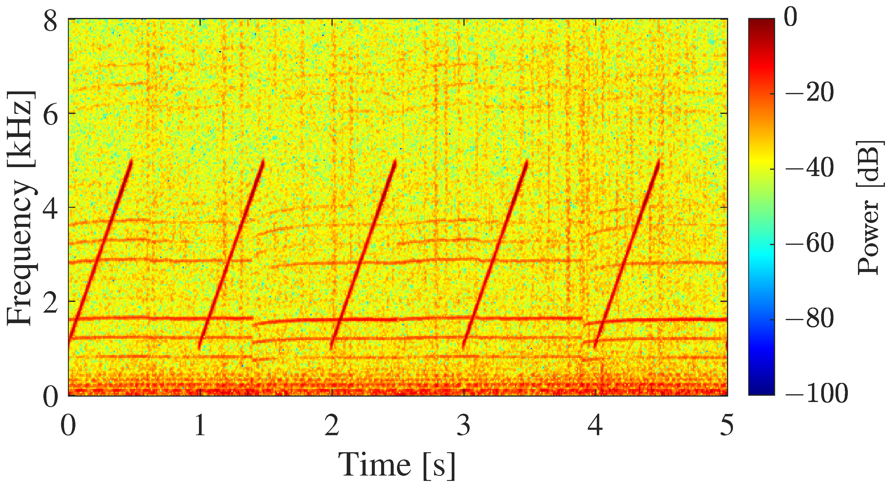
Next, the effect of active acoustic sensing on SSL performance is evaluated. In this evaluation, signals recorded by Sensor 1 during active acoustic sensing, which explicitly include the transmitted sensing signals, are combined with numerically simulated localization target sounds and analyzed using the SSL method. The DOA of the localization target sound is fixed at $(\theta ,\varphi )=(0,-45)$ deg., and the SNR of the localization target sound relative to drone ego-noise is varied from $-20$ to 0 dB. Figure 20 shows an example spectrogram of the signals used for the analysis. A sensing signal with a duration of 0.5 s is transmitted at intervals of 0.5 s, while the localization target sound is continuously present. Because the reflections from the ground surface are relatively weak, it is expected that the direct sound propagating from the sensing speaker (mounted at the center of Sensor 1) to the microphones has a dominant influence on SSL performance.

Figure 21 shows examples of the MUSIC spatial spectrum $\overline{P}$ obtained using Equation (4) for signals with an SNR of $-10$ dB when the localization target sound is a voice signal. Figure 21a shows the result obtained by analyzing time periods during which the sensing signal is transmitted (e.g., 0–0.5 s in Figure 20), whereas Figure 21b shows the result obtained by analyzing time periods without sensing signal transmission (e.g., 0.5–1 s). The spatial spectrum $\overline{P}$ is plotted according to the coordinate system shown in Figure 17, and the power of sounds arriving from each direction is visualized using a colormap. In Figure 21a, a strong high-power component appears near $\varphi =-90$ deg., which is caused by the sensing signal, making the component corresponding to the localization target sound near $(\theta ,\varphi )=(0,-45)$ deg. difficult to observe. In contrast, in Figure 21b, the power of components caused by the sensing signal is significantly reduced, and the component corresponding to the localization target sound becomes clearly observable. Although the direct signal of the sensing signal is not included in the analyzed time periods, it is assumed that components due to multipath reflections between the drone body and the sensor, and internal acoustic reverberation remain and appear near $\varphi =-90$ deg. However, their power is sufficiently smaller than that of the localization target sound, suggesting that their influence on SSL performance is limited when the SNR is high.

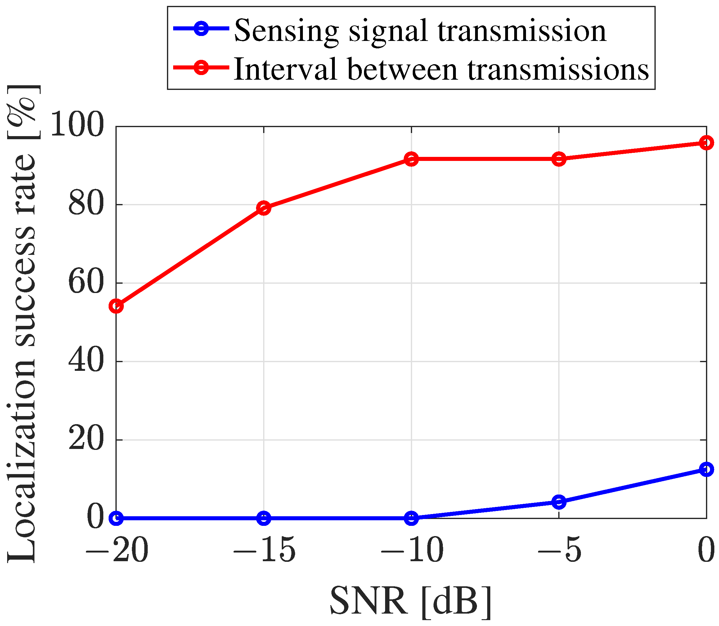
Based on this analysis, the localization performance is evaluated by varying the SNR from $-20$ to 0 dB. For each SNR, 48 trials are conducted, and the localization success rate is calculated in the same manner as in Section 3.2.2 using the results obtained with both voice and whistle target sounds. In the previous evaluation, a larger number of trials could be generated because simulated localization target sounds were used together with recorded drone ego-noise signals. In contrast, the number of trials in the present evaluation is smaller because real sensing signals recorded during active acoustic sensing are used. The duration of these recordings limits the number of available trials. Figure 22 shows the resulting localization success rates, where the horizontal axis represents the SNR and the vertical axis represents the localization success rate. The results obtained during sensing signal transmission are shown by the blue line, while those obtained during intervals without sensing signal transmission are shown by the red line. During the sensing signal transmission, the localization success rate remains below 20% for all SNR conditions. In contrast, during intervals without sensing signal transmission, the success rate is approximately 50% at an SNR of $-20$ dB and exceeds 80% when the SNR is higher than $-15$ dB. These results indicate that SSL can be effectively performed during intervals in which the sensing signal is not transmitted. In practical active acoustic sensing, transmission intervals are inherently required to receive reflected signals from the ground surface. In addition, it is unlikely that localization target sounds exist only during the short periods in which sensing signals are transmitted, and the timing of sensing signal transmission is fully grasped and controlled by the system. Therefore, performing SSL during intervals without sensing signal transmission is considered a practical and effective strategy. These results demonstrate the feasibility of SSL during active acoustic sensing and clarify the influence of SNR on localization performance.

3.2.4. Effect of Sound Source Localization on Acoustic Sensing

Finally, the effect of localization target sounds on active acoustic sensing performance is evaluated. Active acoustic sensing analysis is performed on the same signals as those used in Section 3.2.3, which include both sensing signals and localization target sounds. While SSL performance degrades when the SNR of the localization target sound is low, active acoustic sensing performance is expected to degrade when the localization target sound has a high SNR.

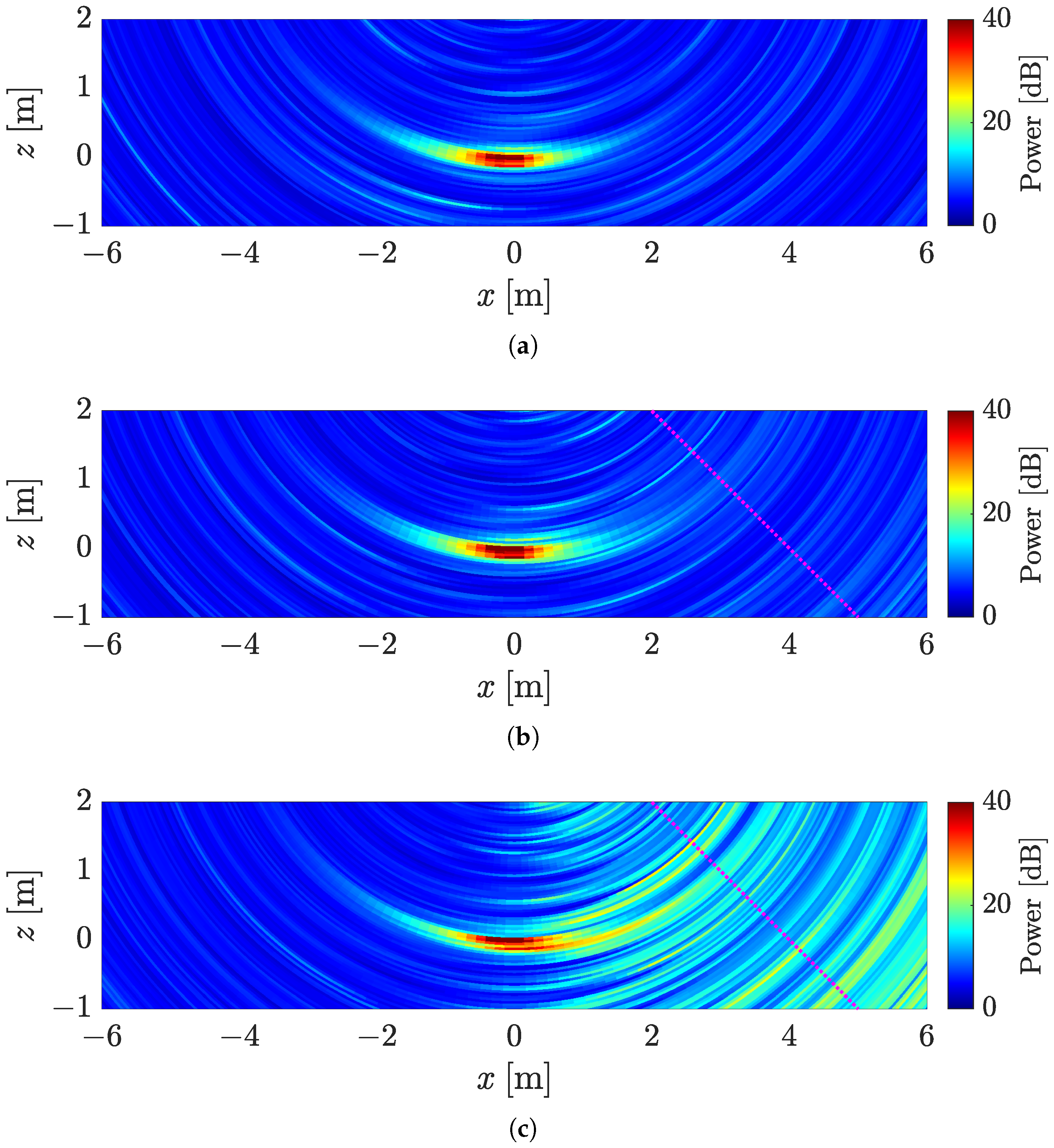
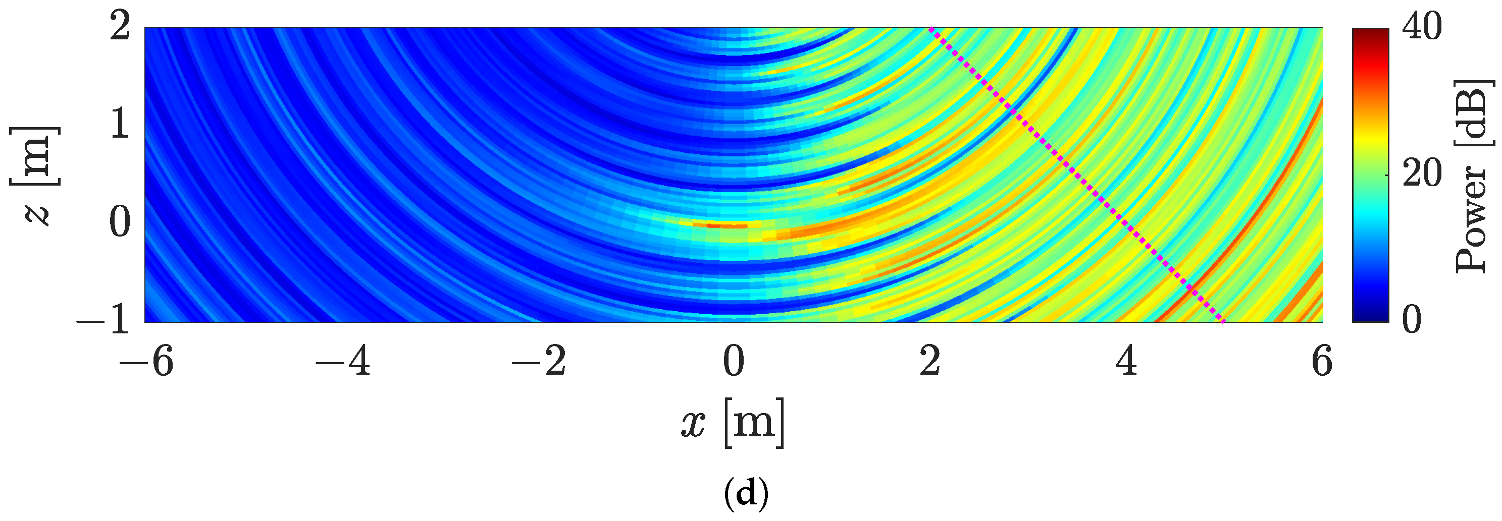
Figure 23 shows examples of two-dimensional cross section of the sensing results, represented by the MUSIC spatial spectrum $\overline{P^{\prime }}$ obtained using Equation (10) when the localization target sound is a voice signal. The sensor position is $(x,y,z)=(0,0,5)$ m, and the results correspond to a cross section at $y=0$ m. Figure 23a shows the result without localization target sounds, while Figure 23b–d show the results when the SNR of the localization target sound is $-20$, $-10$, and 0 dB, respectively. The DOA of the localization target sound is indicated by a magenta dotted line. When the SNR is $-20$ dB, the influence of the localization target sound is limited, and the sensing result is similar to that obtained without localization target sounds. A clear component corresponding to the ground surface can be observed near $(x,z)=(0,0)$ m, directly beneath the sensor. When the SNR increases to $-10$ dB, components caused by the localization target sound appear in the region $x>0$. At an SNR of 0 dB, these components become dominant, making it difficult to distinguish the ground surface components.

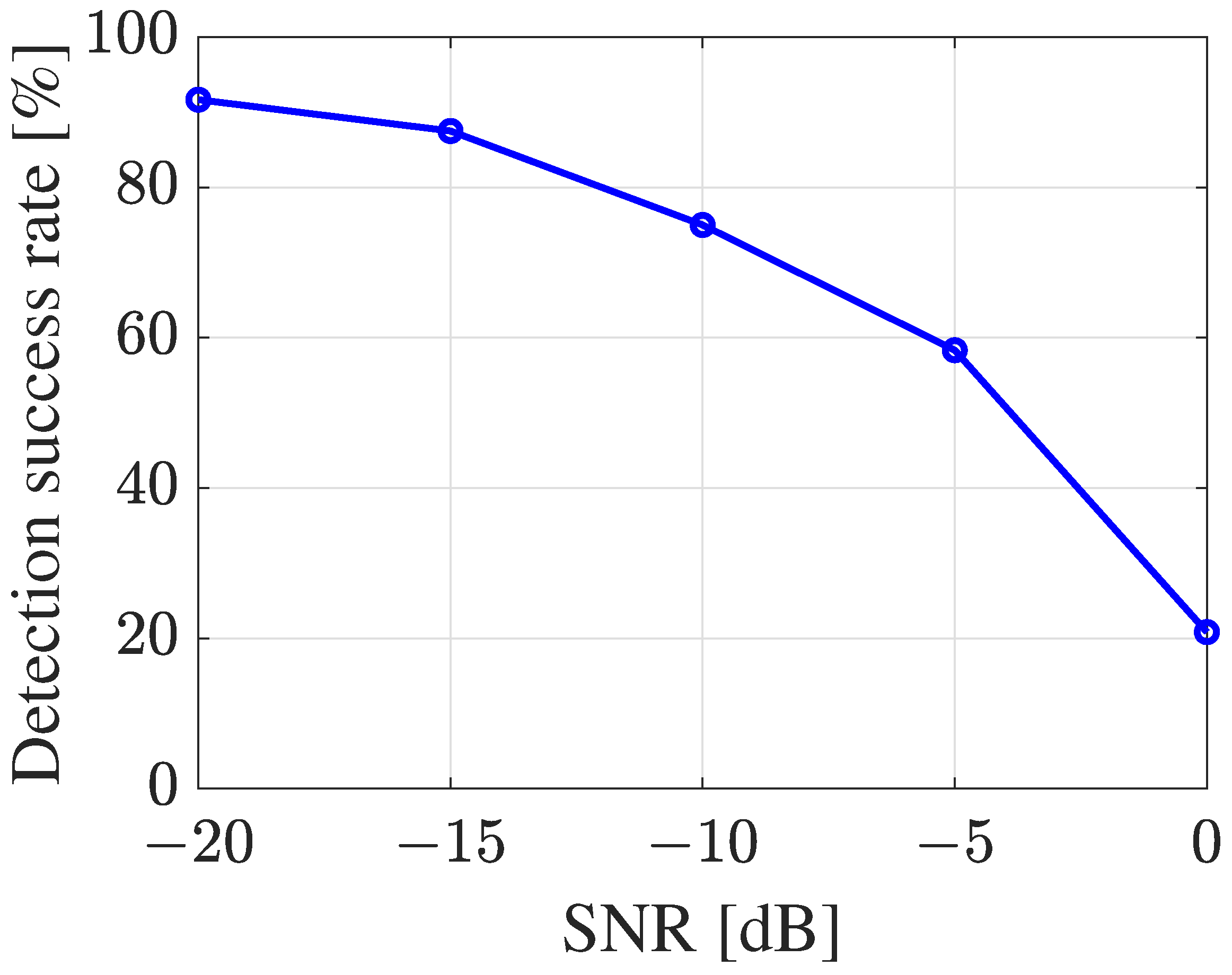
To quantitatively evaluate this effect, the SNR is varied from $-20$ to 0 dB, and 24 trials are conducted for each SNR condition. The detection success rate is calculated in the same manner as in Section 3.1.3 using the results obtained with both voice and whistle target sounds. Figure 24 shows the resulting detection success rates, where the horizontal axis represents the SNR and the vertical axis represents the detection success rate. When the SNR is $-20$ dB, the success rate exceeds 90%. However, as the SNR increases, the success rate decreases, reaching approximately 20% at an SNR of 0 dB. These results indicate that high-power localization target sounds significantly degrade active acoustic sensing performance.

Unlike SSL during active acoustic sensing, where the timing of sensing signal transmission can be precisely grasped and controlled, the timing and power of localization target sounds cannot be controlled in practical scenarios. Therefore, when the SNR of localization target sounds is high, it may be necessary to increase the power of the sensing signal or adjust the drone altitude to reduce the relative SNR of the localization target sound. However, increasing the sensing signal power degrades SSL performance, while increasing the drone altitude reduces both the reflected signal power from the ground surface and the localization target sound power, resulting in degraded sensing and localization performance. These observations reveal a fundamental trade-off between active acoustic sensing performance and SSL performance during simultaneous execution. To maintain both sensing and localization performance, control algorithms that jointly optimize sensing signal parameters and drone positioning are required.

Through these evaluation experiments, the fundamental performance of the proposed active acoustic sensing method and its behavior during simultaneous execution with SSL are clarified, revealing the limitations and challenges of the proposed framework.

4. Conclusions

This paper proposed and experimentally validated an active acoustic sensing method based on the MUSIC framework for estimating ground surface conditions using a drone-mounted speaker and microphone array. The proposed method enables three-dimensional localization of reflection points based on the principle of echolocation and shares both hardware and signal processing components with SSL for victim search. First, the fundamental sensing performance was evaluated in an outdoor environment. The results demonstrated that the proposed method can successfully detect representative ground surface anomalies, including ground surface depressions and cracks. Sensing performance was shown to strongly depend on the transmitted chirp signal parameters, and appropriate signal design was essential for achieving reliable detection under drone-mounted conditions. A frequency range of 1–5 kHz and a duration of 0.5 s were found to provide a suitable balance between SNR improvement and impulse resolution. Second, the influence of sensing position, drone ego-noise, and position and attitude fluctuations was investigated. The effective horizontal sensing range at an altitude of 5 m was approximately 1 m for both depressions and cracks, clarifying the current sensing coverage limitation of the proposed framework. The results further revealed how geometric spreading loss, angular and frequency-dependent reflection characteristics, as well as ego-noise and fluctuations, jointly affect detection performance under different surface conditions. Finally, the feasibility of simultaneous execution of active acoustic sensing and SSL was evaluated. SSL was shown to be effectively performed during intervals between sensing signal transmissions. In contrast, strong localization target sounds degraded sensing performance. These findings clarify the mutual interactions between sensing and localization performance and reveal a fundamental trade-off during simultaneous operation on a single drone platform. Overall, this study provides a practical foundation for integrating environmental surface sensing and victim localization using a unified drone-based acoustic system. Future work includes optimization of sensing signal design and drone positioning strategies to balance sensing and localization performance, extension to other types of surface anomalies, and development of dynamic scanning methods for wider-area coverage.

References

1. World Health Organization. Türkiye Earthquake: External Situation Report no. 4: 6–12 March 2023. Available online: https://www.who.int/europe/publications/i/item/WHO-EURO-2023-7145-46911-68727 (accessed on 2 February 2026).
2. World Health Organization. Whole of Syria: Situation Report, 3–12 March 2023. Available online: https://www.emro.who.int/images/stories/syria/whole-of-syria-sit-rep-6-12-march-2023.pdf (accessed on 2 February 2026).
3. Jang, H.C.; Lien, Y.N.; Tsai, T.C. Rescue information system for earthquake disasters based on MANET emergency communication platform. In Proceedings of the International Conference on Wireless Communications and Mobile Computing (IWCMC), Leipzig, Germany, 21–24 June 2009; pp. 623–627. [Google Scholar] [CrossRef]
4. Murphy, R.R.; Tadokoro, S.; Kleiner, A. Disaster Robotics. In Springer Handbook of Robotics; Springer: Berlin, Germany, 2016; pp. 1577–1604. [Google Scholar] [CrossRef]
5. Tadokoro, S. Disaster Robotics: Results from the ImPACT Tough Robotics Challenge; Springer: Berlin, Germany, 2019; pp. 1–528. [Google Scholar]
6. Baek, J.H.; Choi, J.H.; Kim, S.M.; Park, H.J.; Kuc, T.Y. A Mobile Robot Framework in Industrial Disaster for Human Rescue. In Proceedings of the 22nd International Conference on Control, Automation and Systems (ICCAS), Jeju, Republic of Korea, 27 November–1 December 2022; pp. 623–628. [Google Scholar] [CrossRef]
7. Kamegawa, T.; Akiyama, T.; Sakai, S.; Fujii, K.; Une, K.; Wang, Y.; Matsumura, Y.; Kishutani, T.; Nose, E.; Yoshizaki, Y.; et al. Development of a separable search-and-rescue robot composed of a mobile robot and a snake robot. Adv. Robot. 2020, 34, 132–139. [Google Scholar] [CrossRef]
8. Lyu, M.; Zhao, Y.; Huang, C.; Huang, H. Unmanned Aerial Vehicles for Search and Rescue: A Survey. Remote Sens. 2023, 15, 3266. [Google Scholar] [CrossRef]
9. Quan, A.; Herrmann, C.; Soliman, H. Project Vulture: A Prototype for Using Drones in Search and Rescue Operations. In Proceedings of the 15th International Conference on Distributed Computing in Sensor Systems (DCOSS), Santorini, Greece, 29–31 May 2019; pp. 619–624. [Google Scholar] [CrossRef]
10. Weldon, W.T.; Hupy, J. Investigating Methods for Integrating Unmanned Aerial Systems in Search and Rescue Operations. Drones 2020, 4, 38. [Google Scholar] [CrossRef]
11. Sambolek, S.; Ivasic-Kos, M. Automatic Person Detection in Search and Rescue Operations Using Deep CNN Detectors. IEEE Access 2021, 9, 37905–37922. [Google Scholar] [CrossRef]
12. Tanida, N. What happened to elderly people in the great Hanshin earthquake. BMJ 1996, 313, 1133–1135. [Google Scholar] [CrossRef] [PubMed]
13. Ashkenazi, I.; Isakovich, B.; Kluger, Y.; Alfici, R.; Kessel, B.; Better, O.S. Prehospital management of earthquake casualties buried under rubble. Prehospital Disaster Med. 2005, 20, 122–133. [Google Scholar] [CrossRef] [PubMed]
14. Chevtchenko, S.F.; Rodríguez, B.J.; Vale, R.; Soti, A.; Bethi, Y.; Ibnul, N.; Marcireau, A.; Azghadi, M.R.; Wabnitz, A.; Afshar, S. Drone-Based Sound Source Localization: A Systematic Literature Review. IEEE Access 2025, 13, 94256–94274. [Google Scholar] [CrossRef]
15. Schmidt, R.O. Multiple emitter location and signal parameter estimation. IEEE Trans. Antennas Propag. 1986, 34, 276–280. [Google Scholar] [CrossRef]
16. Hoshiba, K.; Washizaki, K.; Wakabayashi, M.; Ishiki, T.; Kumon, M.; Bando, Y.; Gabriel, D.; Nakadai, K.; Okuno, H.G. Design of UAV-Embedded Microphone Array System for Sound Source Localization in Outdoor Environments. Sensors 2017, 17, 2535. [Google Scholar] [CrossRef]
17. Hoshiba, K.; Nakadai, K.; Kumon, M.; Okuno, H.G. Assessment of MUSIC-Based Noise-Robust Sound Source Localization with Active Frequency Range Filtering. J. Robot. Mechatron. 2018, 30, 426–435. [Google Scholar] [CrossRef]
18. Hoshiba, K.; Komatsuzaki, I.; Iwatsuki, N. Proposal of Practical Sound Source Localization Method Using Histogram and Frequency Information of Spatial Spectrum for Drone Audition. Drones 2024, 8, 159. [Google Scholar] [CrossRef]
19. Wang, L.; Cavallaro, A. Deep Learning Assisted Time-Frequency Processing for Speech Enhancement on Drones. IEEE Trans. Emerg. Top. Comput. Intell. 2021, 5, 871–881. [Google Scholar] [CrossRef]
20. Strauss, M.; Mordel, P.; Miguet, V.; Deleforge, A. DREGON: Dataset and Methods for UAV-Embedded Sound Source Localization. In Proceedings of the IEEE/RSJ International Conference on Intelligent Robots and Systems (IROS), Madrid, Spain, 1–5 October 2018; pp. 1–8. [Google Scholar] [CrossRef]
21. Cheng, M.L.; Matsuoka, M.; Liu, W.; Yamazaki, F. Near-real-time gradually expanding 3D land surface reconstruction in disaster areas by sequential drone imagery. Autom. Constr. 2022, 135, 104105. [Google Scholar] [CrossRef]
22. Suzuki, T.; Inoue, D.; Amano, Y. Robust UAV Position and Attitude Estimation using Multiple GNSS Receivers for Laser-based 3D Mapping. In Proceedings of the IEEE/RSJ International Conference on Intelligent Robots and Systems (IROS), Macau, China, 3–8 November 2019; pp. 4402–4408. [Google Scholar] [CrossRef]
23. Afriansyah, F.L.; Purnomo, F.E.; Fanani, N.Z.; Widiastuti, I.; Muna, N. Altitude Optimization Using Ultrasonic Sensors of Unmanned Aerial Vehicle for Foliar Fertilizer. In Proceedings of the Second International on Food and Agriculture, Bali, Indonesia, 2–3 November 2019; pp. 156–160. [Google Scholar]
24. Su, Y. Experimental study of an ultrasonic low altitude altimetry system for UAVs. In Proceedings of the Third International Conference on Control and Intelligent Robotics (ICCIR), Changsha, China, 23–25 June 2023; pp. 808–813. [Google Scholar] [CrossRef]
25. Wilshin, S.; Amos, S.; Bomphrey, R.J. Seeing with sound; surface detection and avoidance by sensing self-generated noise. Int. J. Micro Air Veh. 2023, 15, 17568293221148377. [Google Scholar] [CrossRef]
26. Nilsson, H.; Rydell, J.; Kullberg, A.; Hendeby, G. Dronar: Obstacle Echolocation Using Drone Ego-Noise. In Proceedings of the IEEE International Conference on Acoustics, Speech, and Signal Processing Workshops (ICASSPW), Seoul, Republic of Korea, 14–19 April 2024; pp. 184–188. [Google Scholar] [CrossRef]
27. Yano, T.; Yen, B.; Nakadai, K. Drone audition: Dataset and methods for ground surface material classification using drone noise in outdoor environment. In Proceedings of the 16th Asia Pacific Signal and Information Processing Association Annual Summit and Conference (APSIPA ASC), Macau, China, 3–6 December 2024; pp. 1–6. [Google Scholar] [CrossRef]
28. Noda, R.; Hirose, M.; Nakata, T.; Liu, H. Low-Noise Propeller Design with Enlarged Blade Area for Drones. J. Robot. Mechatron. 2025, 37, 799–806. [Google Scholar] [CrossRef]
29. Kapoor, R.; Ramasamy, S.; Gardi, A.; Schyndel, R.V.; Sabatini, R. Acoustic Sensors for Air and Surface Navigation Applications. Sensors 2018, 18, 499. [Google Scholar] [CrossRef]
30. Saqib, U.; Jensen, J.R. A framework for spatial map generation using acoustic echoes for robotic platforms. Robot. Auton. Syst. 2022, 150, 104009. [Google Scholar] [CrossRef]
31. Dümbgen, F.; Hoffet, A.; Kolundžija, M.; Scholefield, A.; Vetterli, M. Blind as a Bat: Audible Echolocation on Small Robots. IEEE Robot. Autom. Lett. 2023, 8, 1271–1278. [Google Scholar] [CrossRef]
32. Laurijssen, D.; Daems, W.; Steckel, J. HiRIS: An Airborne Sonar Sensor with a 1024 Channel Microphone Array for In-Air Acoustic Imaging. IEEE Access 2024, 12, 51786–51795. [Google Scholar] [CrossRef]
33. Jansen, W.; Laurijssen, D.; Steckel, J. Stabilized Adaptive Steering for 3D Sonar Microphone Arrays with IMU Sensor Fusion. In Proceedings of the IEEE SENSORS, Kobe, Japan, 20–23 October 2024; pp. 1–4. [Google Scholar] [CrossRef]
34. Angrisani, L.; Moriello, R.S.L. Estimating ultrasonic time-of-flight through quadrature demodulation. IEEE Trans. Instrum. Meas. 2006, 55, 54–62. [Google Scholar] [CrossRef]
35. Blanford, T.E.; Williams, D.P.; Park, J.D.; Reinhardt, B.T.; Dalton, K.S.; Johnson, S.F.; Brown, D.C. An in-air synthetic aperture sonar dataset of target scattering in environments of varying complexity. Sci. Data 2024, 11, 1196. [Google Scholar] [CrossRef]
36. Cook, C.E. Pulse Compression-Key to More Efficient Radar Transmission. Proc. IRE 1960, 48, 310–316. [Google Scholar] [CrossRef]
37. Nonami, K.; Hoshiba, K.; Nakadai, K.; Kumon, M.; Okuno, H.G.; Tanabe, Y.; Yonezawa, K.; Tokutake, H.; Suzuki, S.; Yamaguchi, K.; et al. Recent R&D Technologies and Future Prospective of Flying Robot in Tough Robotics Challenge. In Disaster Robotics; Tadokoro, S., Ed.; Springer: Cham, Switzerland, 2019; pp. 77–142. [Google Scholar] [CrossRef]
38. Nakamura, K.; Nakadai, K.; Asano, F.; Hasegawa, Y.; Tsujino, H. Intelligent sound source localization for dynamic environments. In Proceedings of the IEEE/RSJ International Conference on Intelligent Robots and Systems (IROS), St. Louis, MO, USA, 10–15 October 2009; pp. 664–669. [Google Scholar] [CrossRef]
39. Nakamura, K.; Nakadai, K.; Ince, G. Real-time super-resolution Sound Source Localization for robots. In Proceedings of the IEEE/RSJ International Conference on Intelligent Robots and Systems (IROS), Vilamoura-Algarve, Portugal, 7–12 October 2012; pp. 694–699. [Google Scholar] [CrossRef]
40. Okutani, K.; Yoshida, T.; Nakamura, K.; Nakadai, K. Outdoor auditory scene analysis using a moving microphone array embedded in a quadrocopter. In Proceedings of the IEEE/RSJ International Conference on Intelligent Robots and Systems (IROS), Vilamoura-Algarve, Portugal, 7–12 October 2012; pp. 3288–3293. [Google Scholar] [CrossRef]
41. Ohata, T.; Nakamura, K.; Mizumoto, T.; Tezuka, T.; Nakadai, K. Improvement in outdoor sound source detection using a quadrotor-embedded microphone array. In Proceedings of the IEEE/RSJ International Conference on Robots and Intelligent Systems (IROS), Chicago, IL, USA, 14–18 September 2014; pp. 1902–1907. [Google Scholar] [CrossRef]
Figure 1. Conceptual illustration of active acoustic sensing using a drone-mounted speaker and microphone array. (a) Acoustic signals transmitted from the drone-mounted speaker are reflected at multiple points on the ground surface. (b) An example of acoustic signals recorded by the microphone array, including direct and reflected signals. (c) An example of the obtained spatial spectrum.
Drones 10 00258 g001
Figure 2. Sensors used in the experiments and the drone platform on which they were mounted. (a) Sensor 1, consisting of a speaker and a 16-channel microphone array. The speaker is located at the center of the enclosure, and each microphone is indicated by a red arrow and arranged around the speaker. (b) Drone equipped with the sensors and the processing unit. Sensor 2 is a microphone array for SSL used in the evaluation described in Section 3.2. Sensor 1 is mounted on the lower part of the drone, while Sensor 2 and the processing unit are installed on a pipe attached to the drone.
Drones 10 00258 g002
Figure 3. Experimental setup for the active acoustic sensing evaluation. The sensing targets are a ground surface depression and a ground surface crack located on a flat road surface. The drone performs sensing while hovering at an altitude of 5 m.
Drones 10 00258 g003
Figure 4. Dimensions of the sensing targets. (a) Ground surface depression. (b) Ground surface crack.
Drones 10 00258 g004
Figure 5. Shape of the sensing targets measured using LiDAR, used as a reference for evaluation. (a) Ground surface depression. (b) Ground surface crack.
Drones 10 00258 g005aDrones 10 00258 g005b
Figure 6. Drone hovering positions for each sensing experiment. Sensing is performed from an altitude of 5 m above the positions indicated by blue circles. (a) Ground surface depression. (b) Ground surface crack.
Drones 10 00258 g006aDrones 10 00258 g006b
Figure 7. Example of two-dimensional cross-sectional sensing results of a ground surface depression obtained using different transmitted signals. Sensing is performed from the drone position at ( x , y , z ) = ( 1 , 0 , 5 ) m. The results correspond to a two-dimensional cross section at y = 0 m. The ground surface profile measured using LiDAR is also plotted as a black line for reference. (a) Signal 1. (b) Signal 2. (c) Signal 3.
Drones 10 00258 g007
Figure 8. Example of two-dimensional cross-sectional sensing results of a ground surface crack obtained using different transmitted signals. Sensing is performed from the drone position at ( x , y , z ) = ( 0 , 2 , 5 ) m. The results correspond to a two-dimensional cross section at x = 0 m. The crack location is indicated by magenta circles. (a) Signal 1. (b) Signal 2. (c) Signal 3.
Drones 10 00258 g008
Figure 9. Examples of two-dimensional cross-sectional sensing results of a ground surface depression obtained at different drone hovering positions. The results correspond to a two-dimensional cross section at y = 0 m. The ground surface profile measured using LiDAR is also plotted as a black line for reference. (a) ( x , y , z ) = ( 2 , 0 , 5 ) m. (b) ( x , y , z ) = ( 1 , 0 , 5 ) m. (c) ( x , y , z ) = ( 0 , 0 , 5 ) m. (d) ( x , y , z ) = ( 1 , 0 , 5 ) m. (e) ( x , y , z ) = ( 2 , 0 , 5 ) m.
Drones 10 00258 g009
Figure 10. Examples of two-dimensional cross-sectional sensing results of a ground surface crack obtained at different drone hovering positions while varying the sensor position along the y direction. The results correspond to a two-dimensional cross section at y = 0 m. The crack location is indicated by magenta lines. (a) ( x , y , z ) = ( 2.5 , 0 , 5 ) m. (b) ( x , y , z ) = ( 3.5 , 0 , 5 ) m. (c) ( x , y , z ) = ( 4.5 , 0 , 5 ) m. (d) ( x , y , z ) = ( 5.5 , 0 , 5 ) m.
Drones 10 00258 g010
Figure 11. Examples of two-dimensional cross-sectional sensing results of a ground surface crack obtained at different drone hovering positions while varying the sensor position along the x direction. The results correspond to a two-dimensional cross section at x = 0 m. The crack location is indicated by magenta circles. (a) ( x , y , z ) = ( 0 , 3 , 5 ) m. (b) ( x , y , z ) = ( 0 , 2 , 5 ) m. (c) ( x , y , z ) = ( 0 , 1 , 5 ) m. (d) ( x , y , z ) = ( 0 , 0 , 5 ) m.
Drones 10 00258 g011
Figure 12. Detection success rate for a ground surface depression at different drone hovering positions. (a) Flat road surface. (b) Depression edge. (c) Inside the depression.
Drones 10 00258 g012
Figure 13. Detection success rate for a ground surface crack at different drone hovering positions. (a) Along the x -axis. (b) Along the y -axis.
Drones 10 00258 g013
Figure 14. Sensor 2, consisting of a 16-channel microphone array, indicated by red arrows, arranged in a spherical configuration with a diameter of 110 mm.
Drones 10 00258 g014
Figure 15. Experimental setup for evaluating the simultaneous execution of active acoustic sensing and SSL. The drone hovers at an altitude of 5m above a flat road surface, and acoustic signals are recorded simultaneously using Sensor 1 and Sensor 2. For SSL evaluation, target sounds arriving from various directions are generated using numerical simulations.
Drones 10 00258 g015
Figure 16. Spectrograms of SSL target sounds. (a) Voice. (b) Whistle.
Drones 10 00258 g016
Figure 17. Definition of the azimuth angle θ and elevation angle ϕ used for plotting MUSIC spatial spectra for SSL.
Drones 10 00258 g017
Figure 18. Examples of MUSIC spatial spectra for SSL without active acoustic sensing. The target sound is located at ( θ , ϕ ) = ( 0 , 45 ) deg. (a) Sensor 2. (b) Sensor 1.
Drones 10 00258 g018
Figure 19. Localization success rate for target sounds arriving from different directions. (a) Sensor 2. (b) Sensor 1.
Drones 10 00258 g019
Figure 20. Example spectrogram of the received signals used for evaluating the simultaneous execution of active acoustic sensing and SSL. Chirp signals for active acoustic sensing are received at intervals of 0.5 s, while the SSL target sound continuously arrives at the microphone array.
Drones 10 00258 g020
Figure 21. Examples of MUSIC spatial spectra for SSL during active acoustic sensing. The target sound is located at ( θ , ϕ ) = ( 0 , 45 ) deg. (a) During transmission of the active acoustic sensing signal. (b) During the interval between consecutive sensing signal transmissions.
Drones 10 00258 g021
Figure 22. Localization success rate during active acoustic sensing under different SNR conditions.
Drones 10 00258 g022
Figure 23. Example of two-dimensional cross-sectional sensing results in the presence of a localization target sound. Sensing is performed from the drone position at ( x , y , z ) = ( 0 , 0 , 5 ) m. The results correspond to a two-dimensional cross section at y = 0 m. The DOA of the localization target sound is indicated by a magenta dotted line. (a) No localization target sound. (b) Localization target sound with SNR = 20 dB. (c) Localization target sound with SNR = 10 dB. (d) Localization target sound with SNR = 0 dB.
Drones 10 00258 g023aDrones 10 00258 g023b
Figure 24. Detection success rate when localization target sounds exist under different SNR conditions.
Drones 10 00258 g024