A Physics-Guided Aeromagnetic Interference Compensation Method for Geomagnetic Sensing in GNSS-Denied UAV Swarm Systems

Highlights

What are the main findings?

• A physics-guided multi-branch neural network (PG-TLNet) is proposed to decompose aeromagnetic interference into a physics-constrained linear subspace and a nonlinear residual subspace, enabling structured and interpretable compensation under strong onboard electromagnetic interference.
• Extensive flight experiments under interference amplitudes up to 1000 nT show that PG-TLNet reduces residual errors to the 20–30 nT level, outperforming conventional Tolles–Lawson and neural-network-based compensation methods while maintaining sub-millisecond inference latency (~94 μs per sample) and improving cross-node measurement consistency, thereby supporting swarm-oriented magnetic sensing deployment.

What are the implications of the main findings?

• The integration of structured physical modeling with lightweight deep learning offers a practical pathway toward real-time, embedded interference suppression in electromagnetically complex aerial platforms. The achieved compensation fidelity provides a stable and reliable magnetic sensing foundation for geomagnetic navigation in GNSS-denied environments, where satellite-based positioning is unavailable or unreliable.
• By homogenizing magnetic measurement quality across sensing nodes under identical maneuvering conditions, the proposed framework facilitates cooperative geomagnetic sensing and localization in UAV swarm systems.

Abstract

Geomagnetic navigation is a promising alternative for positioning and localization of UAV swarm systems in GNSS-denied environments. However, strong and heterogeneous electromagnetic interference generated by onboard power, propulsion, and electronic subsystems severely degrades magnetic measurement fidelity, limiting the achievable accuracy of cooperative UAV swarm navigation. To address this challenge, this paper proposes PG-TLNet, a physics-guided aeromagnetic interference compensation framework based on the extended Tolles–Lawson (T–L) model. By integrating onboard state information (current, voltage, and attitude) with magnetic measurements through physics-consistency constraints and a lightweight multi-branch convolutional neural network, the framework enables robust real-time compensation under strong and time-varying interference while remaining suitable for resource-constrained UAV nodes. Experimental validation using multiple scalar magnetometers under heterogeneous interference conditions, with amplitudes up to 1000 nT, shows that PG-TLNet consistently outperforms the conventional T–L model across all sensing nodes, maintaining residual magnetic interference at approximately 0–30 nT under long-duration and highly dynamic operations. The proposed method achieves an improvement ratio (IR) of up to 15 with an end-to-end inference latency below 94 μs. These results indicate that PG-TLNet meets the practical measurement fidelity requirements for geomagnetic navigation in GNSS-denied environments. By ensuring reliable and consistent magnetic measurements at the individual UAV node level, the proposed framework establishes a practical sensing foundation for geomagnetic navigation and distributed magnetic sensing in UAV swarm systems operating in GNSS-denied environments.

1. Introduction

Unmanned Aerial Vehicles (UAVs) have become an important platform for aeromagnetic surveying and geomagnetic navigation due to their low operational cost, flexible deployment, and ability to operate at low altitudes and in complex terrains [1]. Compared with traditional manned airborne surveys, UAV-based magnetic sensing systems enable dense spatial sampling and rapid mission execution, making them attractive for applications such as mineral exploration, environmental monitoring, unexploded ordnance detection, and auxiliary navigation in GNSS-denied environments. Advances in geomagnetic sensing technologies can further expand the potential of large AI models and LLM-enabled UAV systems by improving the reliability of low-level perception for autonomous aerial platforms, enabling distributed surveying, cooperative mapping, and multi-platform sensing in challenging environments [2,3].

However, the compact structure and electric propulsion systems of UAV platforms inevitably introduce strong platform-induced magnetic interference, which significantly degrades the accuracy and reliability of aeromagnetic measurements [4]. In practical UAV systems, magnetometers are often installed inside or close to the airframe due to constraints related to aerodynamics, payload capacity, and system integration [5]. Consequently, magnetic sensors are exposed to multiple interference sources, including attitude-dependent airframe magnetization, onboard electric currents, electronic speed controllers, and maneuver-induced transient electromagnetic effects [6,7,8,9,10,11,12,13,14]. Moreover, UAV platforms exhibit substantial heterogeneity in terms of size, structural configuration, propulsion systems, sensor placement, and onboard equipment. Such heterogeneity leads to highly variable magnetic interference characteristics across different platforms, making platform-specific or offline-calibrated compensation methods difficult to generalize and potentially causing measurement inconsistency in multi-platform geomagnetic sensing systems.

The Tolles–Lawson (T–L) model is the most widely used aeromagnetic compensation method and has demonstrated reliable performance in traditional manned airborne surveys. By representing platform magnetic interference as a linear combination of attitude-related basis functions, the T–L model provides clear physical interpretability and high computational efficiency. However, Gnadt et al. from MIT pointed out that under conditions involving strong time-varying interference and high-dynamic flight maneuvers, the conventional T–L model exhibits significant limitations [15]. Specifically, it struggles to capture nonlinear and transient disturbances induced by electric propulsion systems and rapid maneuvers, and its performance may degrade significantly when the interference intensity becomes severe [16,17,18,19].

To address transient interference, research groups led by Canciani [20] and Siebler [21] at the Air Force Institute of Technology (AFIT), as well as Xu et al. from the Chinese Academy of Sciences [22], proposed Kalman filter–based approaches to dynamically update T–L parameters. Although these methods improve adaptability to time-varying interference, their performance still deteriorates under strong-interference conditions. More recently, data-driven approaches based on machine learning and neural networks have been investigated to enhance aeromagnetic compensation performance [23,24]. Hezel [25], Zhang [26], and Ma [27] demonstrated the feasibility of neural networks for modeling magnetic interference. However, purely data-driven models often lack physical interpretability and robustness, and their generalization capability may be insufficient when operating conditions vary across heterogeneous UAV platforms. In addition, high computational complexity may hinder real-time onboard deployment, which is a critical requirement for practical UAV sensing systems [28,29,30].

Motivated by these challenges, this paper proposes a physics-guided neural network framework based on the Tolles–Lawson model, termed PG-TLNet, for real-time aeromagnetic interference compensation. The proposed approach combines the physical interpretability of the classical T–L model with the nonlinear modeling capability of a lightweight neural network. By jointly exploiting electrical signals (current and voltage), kinematic information, and magnetic measurements, PG-TLNet establishes a physics-guided mapping between platform states and magnetic interference. In this study, multiple scalar magnetometers mounted on a single aerial platform are used to emulate distributed magnetic sensing nodes. This configuration enables controlled evaluation of cross-node compensation consistency while maintaining identical flight dynamics and environmental conditions for all sensors. Such a setup provides a practical approximation of multi-node sensing scenarios relevant to future multi-UAV geomagnetic sensing systems.

The proposed PG-TLNet framework differs from conventional hybrid linear–neural models in three key aspects. First, instead of treating the neural network as a generic residual corrector, the magnetic interference field is explicitly decomposed into a physics-constrained linear subspace and a nonlinear transient subspace. The extended Tolles–Lawson model captures interpretable linear interference components, while the neural network focuses on modeling nonlinear residual disturbances. Second, a physics-aware multi-branch architecture is introduced to separately process magnetic, electrical, and kinematic inputs before fusion, enabling decoupled representation of heterogeneous interference mechanisms. Third, the proposed framework is specifically designed for real-time onboard deployment. With sub-millisecond inference latency, PG-TLNet satisfies the computational requirements of UAV platforms while maintaining robust compensation performance under strong time-varying interference.

The main contributions of this paper are summarized as follows: (1) A physics-guided aeromagnetic interference decomposition framework is proposed, in which the interference field is separated into a linear physical subspace and a nonlinear residual subspace. The extended Tolles–Lawson model captures interpretable linear interference components, while the neural network models nonlinear transient disturbances. (2) A physics-aware multi-branch architecture is developed to model heterogeneous onboard interference sources. Magnetic, electrical, and maneuver-related signals are processed in dedicated branches prior to fusion, enabling decoupled representation of different interference mechanisms. (3) A structured residual-learning strategy is introduced to constrain the neural network to predict only the compensation residual after physical-model regression, improving learning stability and avoiding redundancy between physical and data-driven modeling. (4) Extensive flight experiments demonstrate that the proposed PG-TLNet framework achieves accurate aeromagnetic compensation with sub-millisecond inference latency under strong time-varying interference conditions, indicating its suitability for real-time onboard deployment in UAV platforms.

2. Extended T-L Linear Regression Model

Let the magnetic sensor measurement at time $t$ be denoted as ${\mathbf{B}}_t$, while the desired geomagnetic signal for navigation tasks is denoted as ${\mathbf{B}}_{\mathrm{e}}$. The difference between the two corresponds to the interference magnetic field generated by the carrier platform, ${\mathbf{B}}_{\mathrm{a}}$ [31]. The relationship among these variables can be expressed as:

$$‖{\mathbf{B}}_{\mathrm{e}}‖\approx ‖{\mathbf{B}}_t‖-{\displaystyle \frac{{\mathbf{B}}_{\mathrm{a}}·{\mathbf{B}}_t}{‖{\mathbf{B}}_t‖}}$$

(1)

The unit vector of the total field can be expressed as ${\displaystyle \frac{{\mathbf{B}}_t}{‖{\mathbf{B}}_t‖}}={[cosx,cosy,cosz]}^{\mathrm{T}}={[{\mu }_1,{\mu }_2,{\mu }_3]}^{\mathrm{T}}$, which is measured using a tri-axial fluxgate magnetometer. The Tolles–Lawson (T–L) model, proposed in the 1950s, remains the most widely adopted approach for compensating platform-generated magnetic interference in airborne magnetometry and navigation. In this framework, is regarded as a quasi-static error consisting of three components: the permanent field ${\mathbf{B}}_{\mathrm{p}\mathrm{e}\mathrm{r}\mathrm{m}}$, the induced field ${\mathbf{B}}_{\mathrm{i}\mathrm{n}\mathrm{d}}$, and the eddy-current field ${\mathbf{B}}_{\mathrm{e}\mathrm{d}\mathrm{d}\mathrm{y}}$ [32]. Since the induced and eddy-current terms generally vary slowly with platform attitude and motion, the term “static” refers to the deterministic functional representation of the interference field rather than strict time invariance. In the Tolles–Lawson framework, the platform-generated magnetic interference is modeled through its projection onto the direction of the total magnetic field. Accordingly, the scalar interference term can be expressed as the sum of permanent, induced, and eddy-current components:

$${\displaystyle \frac{{\mathbf{B}}_{\mathrm{a}}·{\mathbf{B}}_t}{‖{\mathbf{B}}_t‖}}={\mathbf{B}}_{\mathrm{p}\mathrm{e}\mathrm{r}\mathrm{m}}+{\mathbf{B}}_{\mathrm{i}\mathrm{n}\mathrm{d}}+{\mathbf{B}}_{\mathrm{e}\mathrm{d}\mathrm{d}\mathrm{y}}={\mathbf{B}}_{\mathrm{i}\mathrm{n}\mathrm{t}\mathrm{e}\mathrm{r}\mathrm{f}}$$

(2)

The permanent magnetic field arises from remanent magnetization of aircraft materials, forming an inherent field that does not vary with the external field. In the body coordinate system, this contribution can be treated as a constant vector. By projecting the constant ${\mathbf{B}}_{\mathrm{p}\mathrm{e}\mathrm{r}\mathrm{m}}$ onto the unit direction ${[{\mu }_1,{\mu }_2,{\mu }_3]}^{\mathrm{T}}$ and introducing unknown coefficients ${\sigma }_i$, the scalar term can be expanded as Equation (6).

$${\mu }_1={\displaystyle \frac{B_x}{‖{\mathbf{B}}_t‖}}={\displaystyle \frac{B_x}{\sqrt{B_x^2+B_y^2+B_z^2}}}$$

(3)

$${\mu }_2={\displaystyle \frac{B_y}{‖{\mathbf{B}}_t‖}}={\displaystyle \frac{B_y}{\sqrt{B_x^2+B_y^2+B_z^2}}}$$

(4)

$${\mu }_3={\displaystyle \frac{B_z}{‖{\mathbf{B}}_t‖}}={\displaystyle \frac{B_z}{\sqrt{B_x^2+B_y^2+B_z^2}}}$$

(5)

$${\mathbf{B}}_{perm}={\sigma }_1{\mu }_1+{\sigma }_2{\mu }_2+{\sigma }_3{\mu }_3$$

(6)

In addition, the external geomagnetic field induces magnetization in ferromagnetic and paramagnetic components, producing a secondary induced field ${\mathbf{B}}_{\mathrm{i}\mathrm{n}\mathrm{d}}$. In the T–L expansion, this contribution appears as a quadratic basis function of the direction cosines, scaled by ${|\mathbf{B}}_t|$, as shown in Equation (7).

$${\mathbf{B}}_{\mathrm{i}\mathrm{n}\mathrm{d}}=‖{\mathbf{B}}_t‖({\sigma }_4{{\mu }_1}^2+{\sigma }_5{{\mu }_2}^2+{\sigma }_6{{\mu }_3}^2+{\sigma }_7{\mu }_1·{\mu }_2+{\sigma }_8{\mu }_1·{\mu }_3+{\sigma }_9{\mu }_2·{\mu }_3)$$

(7)

The eddy-current field arises when a time-varying external magnetic field induces circulating currents in conducting structures. According to the T–L model, this effect can be expressed as Equation (8).

$${\mathbf{B}}_{\mathrm{e}\mathrm{d}\mathrm{d}\mathrm{y}}=‖{\mathbf{B}}_t‖({\sigma }_{10}{\mu }_1·{\mu }_1\prime +{\sigma }_{11}{\mu }_1·{\mu }_2\prime +{\sigma }_{12}{\mu }_1·{\mu }_3\prime +{\sigma }_{13}{\mu }_2·{\mu }_1\prime +{\sigma }_{14}{\mu }_2·{\mu }_2\prime +{\sigma }_{15}{\mu }_2·{\mu }_3\prime {+\sigma }_{16}{\mu }_3·{\mu }_1\prime +{\sigma }_{17}{\mu }_3·{\mu }_2\prime +{\sigma }_{18}{\mu }_3·{\mu }_3\prime )$$

(8)

The complete physical model is summarized in Equation (9).

$$\begin{gathered} {\mathbf{B}}_{\mathrm{i}\mathrm{n}\mathrm{t}\mathrm{e}\mathrm{r}\mathrm{f}}=\underset{\mathrm{p}\mathrm{e}\mathrm{r}\mathrm{m}\mathrm{a}\mathrm{n}\mathrm{e}\mathrm{n}\mathrm{t} \mathrm{m}\mathrm{a}\mathrm{g}\mathrm{n}\mathrm{e}\mathrm{t}\mathrm{i}\mathrm{c} \mathrm{f}\mathrm{i}\mathrm{e}\mathrm{l}\mathrm{d}}{\underbrace{{\sigma }_1{\mu }_1+{\sigma }_2{\mu }_2+{\sigma }_3{\mu }_3}}+\underset{\mathrm{i}\mathrm{n}\mathrm{d}\mathrm{u}\mathrm{c}\mathrm{e}\mathrm{d} \mathrm{f}\mathrm{i}\mathrm{e}\mathrm{l}\mathrm{d}}{\underbrace{‖{\mathbf{B}}_t‖{(\sigma }_4{{\mu }_1}^2+{\sigma }_5{{\mu }_2}^2+{\sigma }_6{{\mu }_3}^2+{\sigma }_7{\mu }_1{\mu }_2+{\sigma }_8{\mu }_1{\mu }_3+{\sigma }_9{\mu }_2{\mu }_3)}} \\ +\underset{eddy-current field}{\underbrace{‖{\mathbf{B}}_t‖({\sigma }_{10}{\mu }_1{\mu }_1^{\prime }+{\sigma }_{11}{\mu }_1{\mu }_2^{\prime }+{\sigma }_{12}{\mu }_1{\mu }_3^{\prime }+{\sigma }_{13}{\mu }_2{\mu }_1^{\prime }+{\sigma }_{14}{\mu }_2{\mu }_2^{\prime }+{\sigma }_{15}{\mu }_2·{\mu }_3^{\prime }+{\sigma }_{16}{\mu }_3{\mu }_1^{\prime }+{\sigma }_{17}{\mu }_3{\mu }_2^{\prime }{+\sigma }_{18}{\mu }_3{\mu }_3^{\prime })}}={\mathit{A}}_{TL}\left(t\right)\mathit{\sigma } \end{gathered}$$

(9)

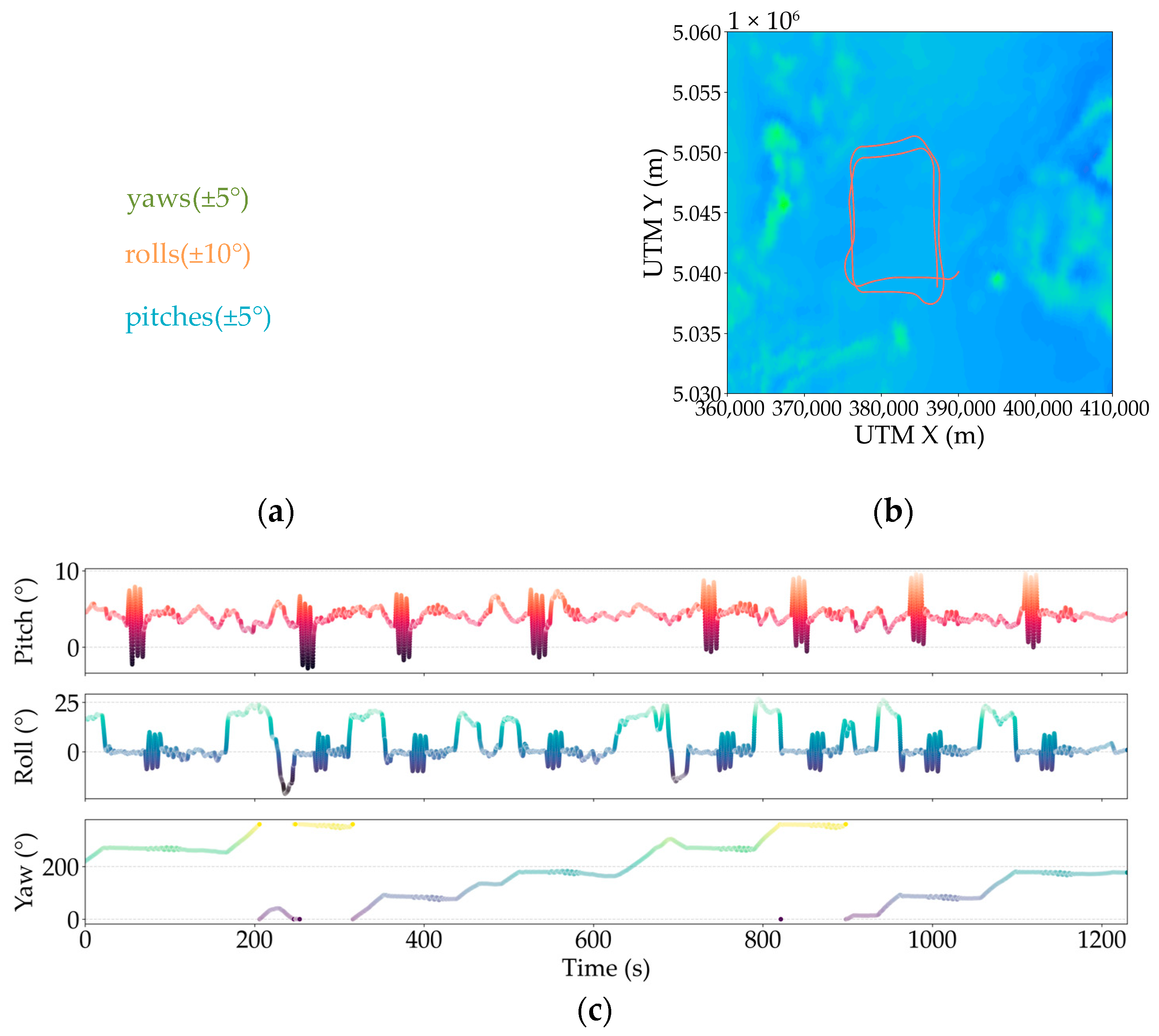
To solve for the coefficient $\mathit{\sigma }$, calibration flights are required. Typically, data are collected through four directional maneuvers [33,34], each including three yaw deflections of ±5°, three roll maneuvers of ±10°, and three pitch maneuvers of ±5°. A schematic of the calibration flight is shown in Figure 1a, and an example of the actual flight trajectory is given in Figure 1b.

To mitigate the ill-conditioned estimation and variance inflation caused by column correlations in the regression matrix, Truncated Singular Value Decomposition (TSVD) with strong robustness is employed for the initial coefficient estimation.

$${\sigma }_k=\sum _{i=1}^k{\displaystyle \frac{u_i·‖{\mathbf{B}}_t‖}{{\alpha }_i}}{v}_i$$

(10)

Here, $u_i$ and $v_i$ denote the left and right singular vectors, respectively, ${\alpha }_i$ is the singular value, and $k$ is the truncation order used to filter out the high-noise directions associated with small singular values, thereby alleviating the ill-posedness caused by multicollinearity. In this study, $k=16$ was selected.

In practical aircraft applications, eddy-current and induced interference are not only related to flight attitude or magnetic field direction, but are also strongly driven by variations in the currents and voltages of onboard electronic devices. The complex coupling among electronics and systems produces interference signals with their own dynamics and time scales, which cannot be fully captured by the T–L model. When carrier-induced interference is relatively weak, the T–L model approximates the geomagnetic field with the measured field [15], as expressed in Equation (1). However, under strong interference, this approximation no longer holds, resulting in model failure. Therefore, it is necessary to augment the T–L model with additional measurable system signal terms.

According to the Biot–Savart law, the magnetic field generated by a current-carrying conductor at the sensor location $\mathit{r}$ can be expressed as:

$$\mathbf{B}\left(\mathbf{r},t\right)={\displaystyle \frac{{\mu }_0}{4\pi }}\oint {\displaystyle \frac{Idl\times \mathbf{R}}{R^3}}$$

(11)

where ${\mu }_0$ denotes the permeability of free space, $I(t)$ is the electric current, $dl$ is the differential element of the conductor, $\mathbf{R}=\mathbf{r}-{\mathbf{r}}^{\prime }$ represents the vector from the current element to the sensor location, and $R = \parallel \mathbf{R}\parallel$. For a fixed conductor geometry and sensor position, the geometric integral depends only on the spatial configuration, while the current $I(t)$ appears as a multiplicative factor. When multiple current loops or current paths with currents $I_1(t),I_2(t),\dots ,I_K(t)$ are present, the total magnetic field measured at the sensor can be expressed as the linear superposition of their individual contributions:

$$\mathbf{B}\left(\mathbf{r},t\right)=\sum _{k=1}^K{I}_k\left(t\right)·({\displaystyle \frac{{\mu }_0}{4\pi }}{\oint }_{C_k}{\displaystyle \frac{Idl\times \mathbf{R}}{R^3}})$$

(12)

Defining the geometric integral as a constant coefficient term:

$${\mathbf{C}}_k\left(\mathbf{r}\right)={\displaystyle \frac{{\mu }_0}{4\pi }}{\oint }_{C_k}{\displaystyle \frac{Idl\times \mathbf{R}}{R^3}}$$

(13)

The magnetic field at the sensor can be written in a compact linear form as:

$$\mathbf{B}\left(\mathbf{r},t\right)=\sum _{k=1}^K{I}_k\left(t\right)·{\mathbf{C}}_k\left(\mathbf{r}\right)$$

(14)

where ${\mathbf{C}}_k\left(\mathbf{r}\right)$ represents an equivalent geometric coupling vector determined by the conductor geometry and sensor location. In practice, this coupling term is generally unknown or difficult to measure directly due to complex wiring layouts and structural configurations. However, in real airborne platforms, effects such as eddy currents, electromagnetic shielding, and structural damping introduce temporal delays and memory effects in the current-to-magnetic-field coupling. These dynamic effects cannot be adequately captured by the static relationship in Equation (14). To account for such behavior, the coupling between the k-th current and the measured magnetic field is modeled as the response of a linear time-invariant (LTI) system driven by the input current. This assumption represents a first-order approximation of the current–magnetic-field coupling under normal operating conditions, where saturation, hysteresis, and temperature-induced nonlinearities are relatively small compared with the dominant interference components. Residual nonlinear effects that cannot be captured by this LTI approximation are subsequently handled by the neural residual-learning module. Denoting the impulse response of the k-th current path as $h_k(\tau )$, which characterizes the dynamic coupling between the current input and the induced magnetic field. In practice, the effective parameters associated with this coupling are implicitly estimated during model training. The total current-induced magnetic interference can then be expressed as:

$$\mathbf{B}\left(t\right)=\sum _{k=1}^K\left(h_k·I_k\right)\left(t\right)=\sum _{k=1}^K{\int }_0^{\infty }{h}_k\left(\tau \right)I_k\left(t-\tau \right)d\tau$$

(15)

where $h_k\left(\tau \right)$ denotes the impulse response describing the current-to-field coupling of the k-th electrical path. Treating the convolution response of each current channel as a system feature, the measured response feature associated with the $k$-th current path is defined as:

$$a_{meas, k}\left(t\right)\triangleq {\int }_0^{\infty }{h}_k\left(\tau \right)I_k\left(t-\tau \right)d\tau$$

(16)

and the corresponding system signal feature vector is constructed as:

$${\mathbf{A}}_{\mathrm{m}\mathrm{e}\mathrm{a}\mathrm{s}}\left(t\right)=\left[a_{meas, 1}\left(t\right), a_{meas, 2}\left(t\right),\dots ,a_{meas, k}\left(t\right)\right]$$

(17)

The overall magnetic interference field is assumed to be a linear combination of the Tolles–Lawson (T–L) terms and the current-induced responses. By augmenting the T–L model with system signal features, the extended interference model can be expressed as:

$${\mathbf{B}}_{\mathrm{i}\mathrm{n}\mathrm{t}\mathrm{e}\mathrm{r}\mathrm{f}}\left(t\right)={\mathbf{A}}_{\mathrm{T}\mathrm{L}}\left(t\right)\mathit{\sigma }+{\mathbf{A}}_{\mathrm{m}\mathrm{e}\mathrm{a}\mathrm{s}}(t)\mathit{\gamma }$$

(18)

Here, ${\mathbf{A}}_{\mathrm{m}\mathrm{e}\mathrm{a}\mathrm{s}}(t)$ consists of functions constructed from the measured onboard currents and their combinations, while $\mathit{\gamma }$ represents the unknown coupling parameters characterizing the linear mapping from system currents to magnetic interference. These parameters are updated online using recursive least squares (RLS), enabling adaptive modeling of induced and eddy-current interference under time-varying operating conditions. Treating system signals as known time-varying inputs yields an engineerable, interpretable, and online-updatable formulation of the current-induced interference term ${\mathbf{A}}_{\mathrm{m}\mathrm{e}\mathrm{a}\mathrm{s}}(t)\mathit{\gamma }$.

3. Proposed Method

The extended Tolles–Lawson (T–L) linear regression model can effectively suppress physically interpretable linear interference components. However, under strong platform-induced interference and high-dynamic operating conditions, complex nonlinear, time-varying, and partially unobserved residuals often remain. These residuals cannot be adequately captured by fixed-basis linear models and often lead to performance degradation in real-time applications. Neural networks are well suited for modeling such residual interference, as they can automatically extract nonlinear features from local temporal patterns, capture short-term temporal coupling, and be efficiently deployed on embedded computing platforms. Importantly, learning these residual components at the single-sensor level enables each aerial platform to provide stable and consistent magnetic measurements, which is a prerequisite for cooperative geomagnetic navigation in UAV swarm systems.

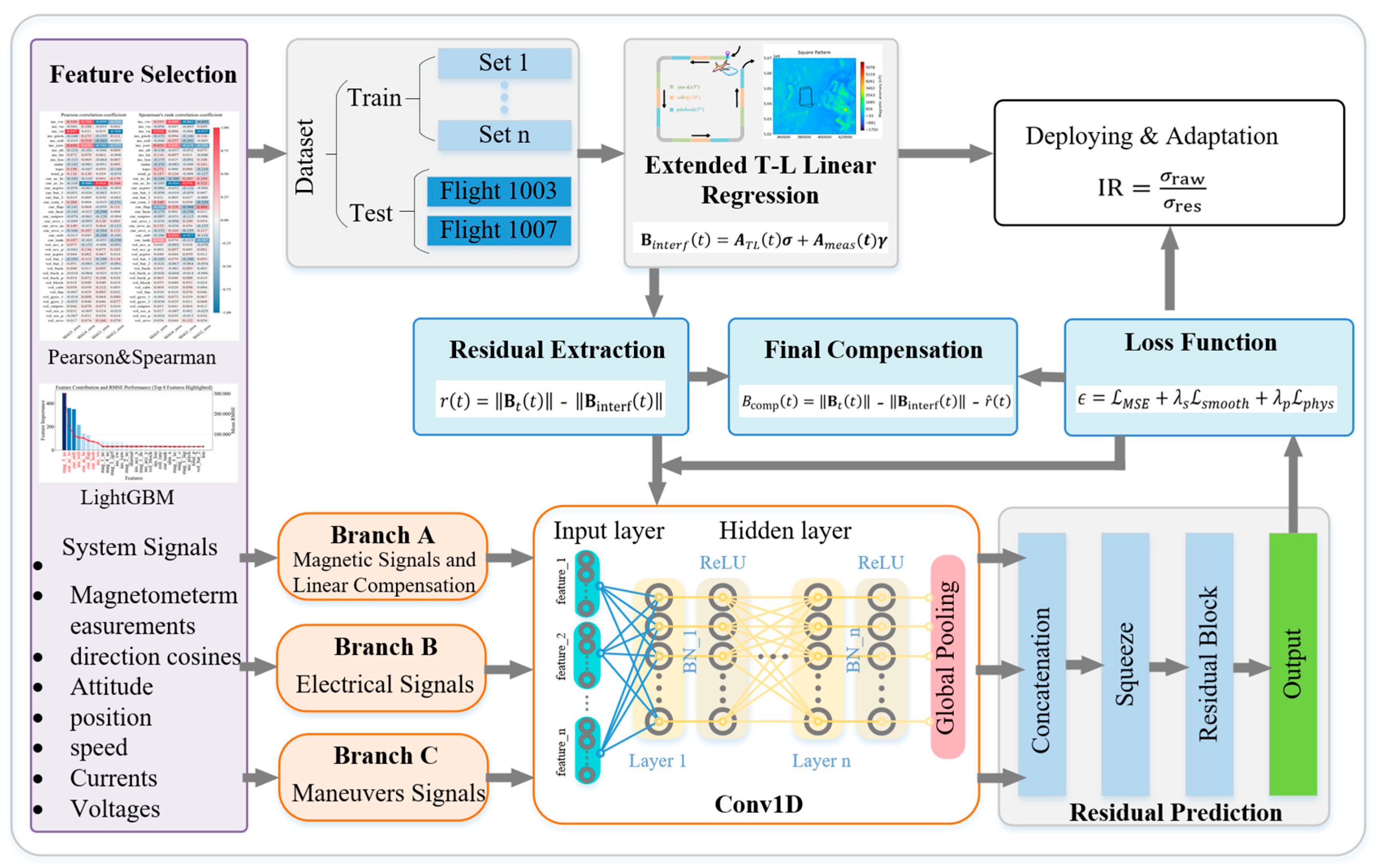
Motivated by this consideration, and inspired by physics-guided neural modeling, this study proposes a real-time, adaptive, and robust aeromagnetic interference compensation framework under strong interference conditions. The proposed method integrates physics-consistent linear modeling with lightweight neural networks to achieve reliable single-sensor compensation, thereby providing a sensing foundation that supports cooperative deployment across UAV swarm systems, as illustrated in Figure 2. Inputs include magnetometer measurements, direction cosines, system signals (currents, voltages), INS signals. Extended TL regression removes the linear errors, and the residual errors is fed into a multi-branch CNN that extracts magnetic, electrical, and kinematic features. The fused CNN prediction is combined with extended TL regression model to yield the final compensated field. Evaluation metrics include the standard deviation (STD) of the residual magnetic field and the improvement ratio (IR $={\displaystyle \frac{{\sigma }_{\mathrm{r}\mathrm{a}\mathrm{w}}}{{\sigma }_{\mathrm{r}\mathrm{e}\mathrm{s}}}}$).

3.1. PG-TLNet Compensation Model

In the PG-TLNet framework, the extended T–L regression model is constructed to compensate for the linear errors corresponding to physically interpretable components (permanent, induced, and eddy-current terms). By incorporating measurable signals (e.g., currents, voltages, positions, velocities) into the induced and eddy-current terms, the remaining residuals can be isolated. To ensure real-time applicability on embedded systems, the neural network is trained only on these residuals, which reduces the function complexity that must be learned by the network and improves training stability. A multi-branch 1D-CNN with embedded physical constraints is employed to learn the nonlinear and time-varying characteristics of the residuals in parallel. The overall workflow of the proposed PG-TLNet method, including both the training and real-time compensation procedures, is summarized in Algorithm 1.

Algorithm 1. Workflow of the algorithm

Data:         1. Training dataset $B_{\mathrm{train}}$ loader         2. Test dataset $B_{\mathrm{test}}$ loader       Output: Compensated magnetic field ${\widehat{B}}_e\left(t\right)$       Training         3. Get $B_{\mathrm{interf}}\left(t\right)$ by extended T–L regression on $B_{\mathrm{train}}$.         4. Compute residual $r\left(t\right)=B_t\left(t\right)-B_{\mathrm{i}\mathrm{n}\mathrm{t}\mathrm{e}\mathrm{r}\mathrm{f}}\left(t\right)$.         5. Get features and branch assignment from Feature Selection section.         6. For epoch = 1:$n$ do         7. Get the predict residual errors $\widehat{r}$ from the multi-branch 1D-CNN network;         8. If $\widehat{r}\in ϵ={\mathcal{L}}_{MSE}+{\lambda }_s{\mathcal{L}}_{smooth}+{\lambda }_p{\mathcal{L}}_{phys}$         9.      |No: ${\widehat{B}}_e\left(t\right)=B_t\left(t\right)-B_{interf}\left(t\right)$         10.    |Yes: ${\widehat{B}}_e\left(t\right)=B_t\left(t\right)-B_{interf}\left(t\right)-\widehat{r}\left(t\right)$         11. | update the value $B_e\left(t\right)$ with ${\widehat{B}}_e\left(t\right)$;         12. | $k=k+1$;         13. End       Testing (Real-Time Compensation)         14. Get $B_{\mathrm{interf}}\left(t\right)$ by extended T–L on $B_{\mathrm{test}}$.         15. Predict residual $\widehat{r}(t)$ with the trained multi-branch 1D-CNN.         16. Condition check (gated correction)         17. Real-time compensation         18. Do reconstruction and get the Compensation value ${\widehat{B}}_e\left(t\right)$           Output: ${\widehat{B}}_e(t)$

Because the inputs are multimodal time-series signals (magnetic measurements, T–L basis functions, currents/voltages, IMU outputs, velocities/positions), preprocessing is first performed to align all features with the magnetometer timeline. High-frequency signals are downsampled to match the magnetometer frequency. By fitting coefficients, the first-order correction $B_{\mathrm{i}\mathrm{n}\mathrm{t}\mathrm{e}\mathrm{r}\mathrm{f}}\left(t\right)$ is obtained, and the residual can be expressed as:

$$r\left(t\right)=B_t\left(t\right)-B_{\mathrm{i}\mathrm{n}\mathrm{t}\mathrm{e}\mathrm{r}\mathrm{f}}\left(t\right)$$

(19)

Residual effects that cannot be linearized are predicted by the neural network. Using a sliding-window approach, magnetometer data, attitude cosines, current/voltage signals, IMU data, and position/velocity measurements are organized as inputs, with a window length of 40 samples (corresponding to approximately 4 s at the 10 Hz sampling rate), which is sufficient to capture transient disturbances during typical maneuvering conditions. To avoid redundant input dimensions, maintain structural clarity, and leverage the temporal convolution capability of CNNs, features are divided into three input branches based on physical attributes and correlations. Each branch undergoes convolution and dimensionality reduction before feature fusion, ensuring both decoupling and interpretability:

Branch A: Magnetic and T–L features. Includes raw magnetometer readings, direction cosines, attitude angles, and the residuals predicted by the extended T–L model with system signal terms. These low-dimensional, physically interpretable features enable the compensation network to capture variations in magnetic disturbances with attitude.

Branch B: Electrical system features. Comprises currents, voltages, RPM, and other features strongly correlated with residuals, along with key lag terms. As these are high-dimensional and redundant, embedding is applied for compression. This branch captures periodic and abrupt interference patterns.

Branch C: Kinematic features. Includes selected current, voltage, velocity, and position features with strong cross-correlation to residuals, reflecting dynamic eddy-current effects. This branch allows the network to recognize coupled patterns during transient maneuvers.

ReLU activation is adopted in this work due to its computational efficiency and stable performance in real-time embedded implementations. Each branch consists of an independent Conv1D, BatchNorm, ReLU, Pooling module to extract local temporal patterns. Global pooling compresses each branch output into a fixed-dimensional vector. Finally, the three branches are concatenated and passed through a residual fully connected layer, with the output layer producing the predicted residual $\widehat{r}\left(t\right)$. The final compensation result is expressed as:

$$B_{\mathrm{c}\mathrm{o}\mathrm{m}\mathrm{p}}\left(t\right)=B_t\left(t\right)-B_{\mathrm{i}\mathrm{n}\mathrm{t}\mathrm{e}\mathrm{r}\mathrm{f}}\left(t\right)-\widehat{r}\left(t\right)$$

(20)

After predicting the residual in each batch, a physics-informed loss function is used to compute the training objective. The total loss is given by:

$$ϵ={\mathcal{L}}_{\mathrm{M}\mathrm{S}\mathrm{E}}+{\lambda }_{\mathrm{s}}{\mathcal{L}}_{\mathrm{s}\mathrm{m}\mathrm{o}\mathrm{o}\mathrm{t}\mathrm{h}}+{\lambda }_{\mathrm{p}}{\mathcal{L}}_{\mathrm{p}\mathrm{h}\mathrm{y}\mathrm{s}}$$

(21)

$${\mathcal{L}}_{\mathrm{M}\mathrm{S}\mathrm{E}}={\displaystyle \frac{1}{N}}\sum _{t=1}^N{(\widehat{r}(t)-r(t))}^2$$

(22)

$${\mathcal{L}}_{\mathrm{s}\mathrm{m}\mathrm{o}\mathrm{o}\mathrm{t}\mathrm{h}}={\displaystyle \frac{1}{N-1}}\sum _{t=2}^N{(\widehat{r}(t)-\widehat{r}(t-1))}^2$$

(23)

$${\mathcal{L}}_{\mathrm{p}\mathrm{h}\mathrm{y}\mathrm{s}}=\sum _t\sum _k{({\displaystyle \frac{\partial \widehat{r}\left(t\right)}{\partial I_k\left(t\right)}}-\gamma )}^2$$

(24)

${\mathcal{L}}_{\mathrm{M}\mathrm{S}\mathrm{E}}$ is the mean squared error between predicted and true residuals, ensuring stable convergence. ${\mathcal{L}}_{\mathrm{s}\mathrm{m}\mathrm{o}\mathrm{o}\mathrm{t}\mathrm{h}}$ is the smoothness constraint that enforces the slow-varying nature of physical magnetic fields and suppresses high-frequency jitter. ${\mathcal{L}}_{\mathrm{p}\mathrm{h}\mathrm{y}\mathrm{s}}$ is the physical consistency constraint to reduce spurious correlations. If the network learns correct physical laws, the predicted residual’s variation with current should conform to Ampère’s law, with $\gamma$ representing the linear current-to-field coupling coefficient. The weights are set as ${\lambda }_{\mathrm{s}}=0.01$ and ${\lambda }_{\mathrm{p}}=0.001$, adjustable depending on the dataset. For training, the AdamW optimizer is employed, with weight pretraining used to shorten convergence time. A LambdaLR scheduler progressively decreases the learning rate across iterations. After each batch, gradients are cleared, the loss is backpropagated, and model weights are updated. To ensure robustness in practical deployment, the framework retains the linear T–L compensation as a fallback solution when the neural network output becomes unreliable.

It is important to emphasize that the neural network does not attempt to relearn the linear interference components already captured by the extended T–L model. Instead, the extended T–L regression first removes physically interpretable linear contributions, including permanent, induced, and current-related linear effects. The CNN is then trained exclusively on the residual term, which predominantly contains nonlinear, time-varying, and higher-order coupling components.

This residual-learning strategy prevents redundancy between the linear regression and the neural network. From a functional decomposition perspective, the model separates interference into a linear subspace (modeled explicitly by physics) and a nonlinear residual subspace (learned by the CNN). The two components are therefore complementary rather than overlapping.

3.2. Feature Selection

The raw input features consist of a large number of variables that may be either strongly cross-correlated or weakly related to magnetic interference. Without feature selection, redundant inputs can cause the model to repeatedly learn overlapping information, leading to increased training complexity, longer convergence time, and reduced interpretability. Moreover, irrelevant or noisy features may induce spurious correlations in convolutional neural networks (CNNs), thereby degrading compensation accuracy and robustness, particularly under strong interference conditions.

To enable lightweight deployment and reliable real-time performance on resource-constrained aerial platforms, the compensation network should focus on learning physically meaningful interference mechanisms rather than incidental noise. Accordingly, this study investigates feature selection for aeromagnetic interference compensation under strong interference conditions and proposes a systematic approach to identify an optimal and compact feature subset. The objective is to achieve a balance between compensation accuracy and computational efficiency, ensuring that sufficient information is retained to capture interference dynamics while minimizing redundancy and noise. By constructing a compact and representative feature set, the risk of overfitting is reduced and the generalization capability across heterogeneous operating conditions is enhanced.

Following the principle of high correlation with the target residual and low mutual redundancy among features, a set of candidate core features is first identified through correlation analysis. Pearson correlation is employed to quantify linear dependence, while Spearman correlation is used to assess monotonic relationships that may not be strictly linear. The minimally interfered tail-stinger magnetometer is used as an approximate reference value. the selected features and their physical interpretations are summarized in

Table 1. T Feature descriptions.

Feature	Description	Unit/Type
ins_vw	west velocity	m/s
ins_vu	vertical velocity	m/s
ins_vn	north velocity	m/s
ins_yaw	computed aircraft yaw	deg
ins_roll	computed aircraft roll	deg
ins_pitch	aircraft pitch	deg
ins_alt	altitude	m
ins_lat	latitude	m
vol_block	voltage: block	V
vol_bat_1	voltage: battery 1	V
vol_bat_2	voltage: battery 2	V
vol_cabt	voltage: cabinet	V
cur_ac_lo	current: air conditioner fan low	A
cur_ac_hi	current: air conditioner fan high	A
cur_flap	current: flap motor	A
cur_heat	current: INS heater	A
cur_srvo_o	current: INS outer servo	A
cur_srvo_i	current: INS internal servo	A
cur_strb	current: strobe lights	A
cur_acpwr	current: system output power	A

. Features with scores ranked within the top 60% are retained for the subsequent step.

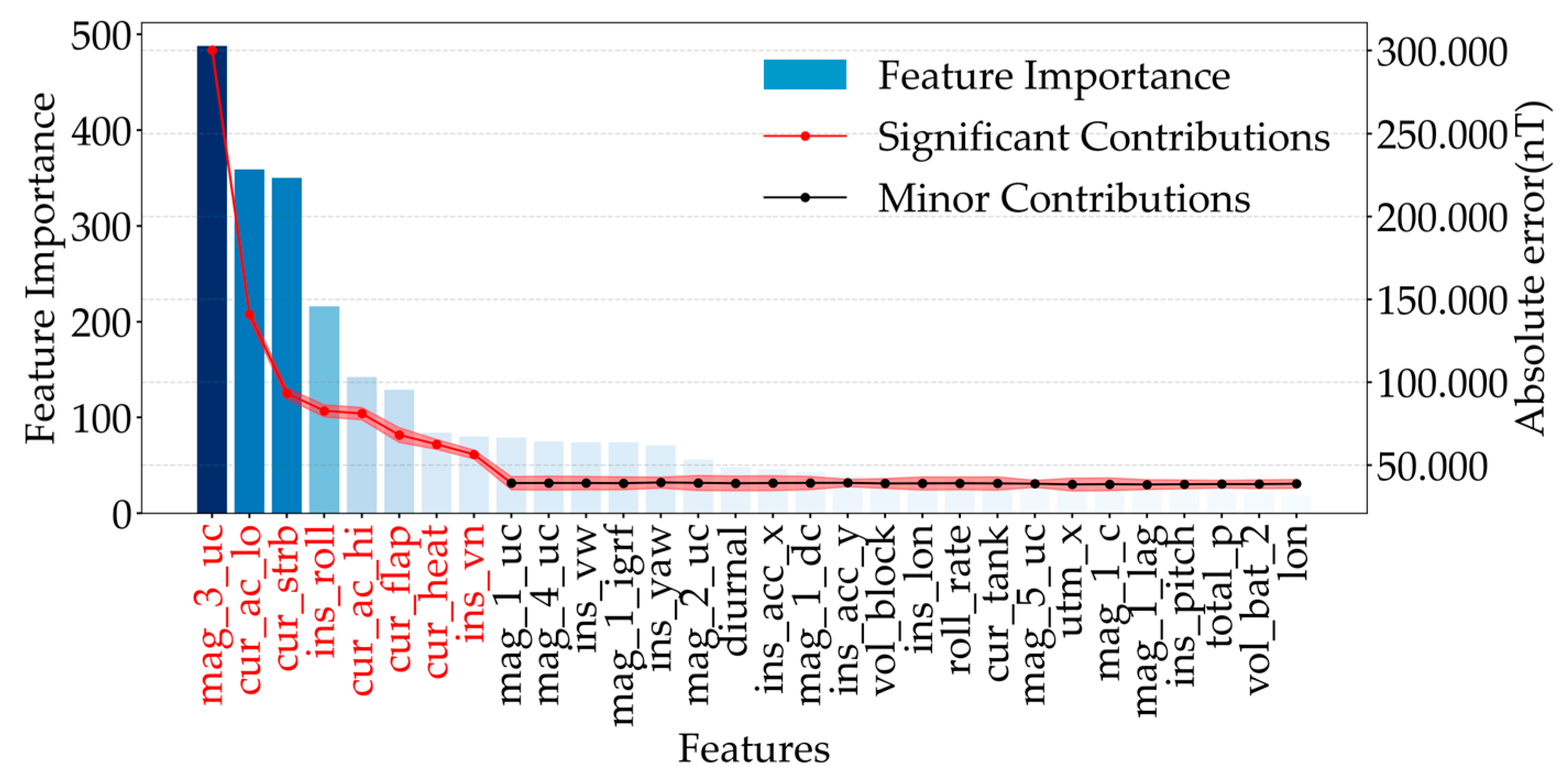
In the next step, a tree-based model (LightGBM) was employed to evaluate the contribution of each feature to interference prediction. A total of 50 independent runs were conducted, and feature ranking was obtained using permutation importance. Features that consistently ranked in the bottom 10% were discarded. The results are shown in Figure 3, where the contribution of each feature is proportional to the height of the corresponding histogram bar, and deeper colors indicate higher feature importance. The red line illustrates the change in cumulative model error with respect to the selected features. At the first eight features, the curve drops sharply, indicating that these features contribute substantially to magnetic interference. Beyond this point, the curve flattens, showing that the remaining features contribute relatively little. The LightGBM analysis indicated that several features from the preliminary screening—including cur_ac_lo, cur_strb, ins_roll, cur_ac_hi, cur_flap, cur_heat, and ins_vn—make significant contributions to compensation performance (highlighted in red), representing the most informative subset. Features such as ins_vw, ins_yaw, ins_pitc, cur_tank, vol_block, and vol_bat_2 (highlighted in black) also showed some predictive contribution.

4. Results

4.1. Data Description

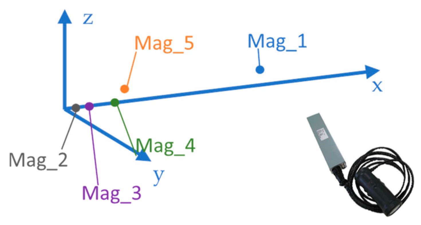
To characterize the variables in this study, a large airborne platform was used as the experimental platform. Five scalar magnetometers were installed at different positions on the platform to simulate sensors operating under different interference environments. Multiple flight segments were used to emulate swarm magnetic sensing nodes. This configuration allows the sensors to experience different local interference conditions while sharing the same flight trajectory and maneuvering state. Such an experimental setup enables a controlled evaluation of the proposed compensation framework. Since the objective of this work is to assess magnetic interference compensation performance, it is important to eliminate additional uncertainties caused by different flight dynamics. Deploying all sensors on the same aerial platform ensures identical maneuvering conditions and environmental exposure, thereby allowing a fair comparison of compensation performance across sensing nodes. This design therefore provides a controlled experimental environment to investigate node-level magnetic measurement consistency, which is a key prerequisite for future multi-UAV geomagnetic sensing and cooperative navigation systems. Among all sensors, Mag_1 is located relatively far from the major onboard interference sources and therefore experiences the smallest platform-induced magnetic disturbance. In this study, Mag_1 is used as an approximate reference measurement. In contrast, Mag_3 is located inside the platform cabin and is close to dense electronic subsystems, where it experiences severe magnetic interference. The interference amplitude can reach approximately 1000 nT. Therefore, Mag_3 is selected as the primary sensor to evaluate the robustness of the proposed method under strong interference conditions. In addition, the vector magnetometer Flux_1 is used to provide vector magnetic field information for constructing the TL compensation model.

The spatial distribution of the magnetometers on the experimental platform is illustrated in Figure 4. A consolidated summary of the onboard magnetometers, including sensor type, sampling rate, and qualitative interference level, is provided in

Table 2. Summary of onboard magnetometers and their interference environments.

Sensors	Type	Sampling Rate	Interference Level
Mag_1	Scalar	10 Hz	☆
Mag_2	Scalar	10 Hz	☆☆☆
Mag_3	Scalar	10 Hz	☆☆☆☆
Mag_4	Scalar	10 Hz	☆☆
Mag_5	Scalar	10 Hz	☆
Flux_1	Vector	10 Hz	☆☆☆☆☆

. The interference level is qualitatively ranked according to the observed amplitude of platform-induced magnetic disturbances during flight experiments, the stars represent the relative level of interference, with a higher number of stars indicating stronger interference. In addition to magnetic measurements, the dataset also includes multiple auxiliary signals describing the operating state of the platform, such as onboard current, voltage, flight attitude, and kinematic variables. A detailed description of the dataset fields is given in

Table 3. Description of the dataset.

Feature Name	Sampling Rate	Description
Magnetometers	10 Hz	Measurements from magnetometers
Current	10 Hz	Onboard current information
Voltage	10 Hz	Onboard voltage information
Attitude	10 Hz	Aircraft orientation angles: yaw, pitch, and roll
Flight Status	10 Hz	Kinematic characteristics of aircraft under various events
Time stamp	10 Hz	Temporal markers for time-series prediction

. All scalar magnetometers operate at a sampling frequency of 10 Hz (0.1 s time interval), ensuring consistent temporal resolution across the sensing nodes. To guarantee proper temporal alignment among heterogeneous signals, all sensor measurements are synchronized using the onboard flight computer timestamp. Electrical signals, attitude measurements, and kinematic data are aligned to the magnetometer timeline prior to model training. Signals with higher sampling rates are downsampled, while lower-rate signals are interpolated to maintain temporal consistency across all input channels.

It should be noted that the dataset adopted in this study spans a wide range of interference sources and dynamic operating conditions. This therefore provides representative and conservative engineering evidence for the potential applicability of the proposed approach across heterogeneous aerial platforms, including UAV and UAV swarm systems. Prior to interference compensation, all sensor data are temporally synchronized, and Z-score normalization is applied to mitigate the influence of differing physical units and numerical scales on model training. All experiments are conducted on a workstation equipped with the CPU (AMD Ryzen 7 7800X3D) is from Advanced Micro Devices (AMD), Santa Clara, CA, USA, and the GPU (NVIDIA GeForce RTX 4060 Ti) is from NVIDIA Corporation, Santa Clara, CA, USA. The proposed algorithm is implemented in Python 3.7 using the PyTorch deep learning framework.

4.2. Results Under Strong Interference Conditions

To validate the effectiveness of the proposed PG-TLNet interference compensation method under strong platform-induced magnetic interference, the flight trajectory dataset was divided into training and testing subsets, as summarized in

Table 4. Summary of flight lines used for training and testing.

Flight Line	Duration	Description
Flt_3	16,000 s	Test set
Flt_4	7968 s	Train set
Flt_5	8017 s	Train set
Flt_6	9905 s	Train set
Flt_7	11,532 s	Test set

. Considering that Flt_3 and Flt_7 have longer durations, traverse more complex geomagnetic environments, and involve more aggressive maneuvering, these flights exhibit significantly stronger and more dynamic magnetic interference. They were therefore selected as independent test sets to rigorously evaluate model performance under severe interference conditions. The segment durations are summarized in Table 4. The remaining flights (Flt_4, Flt_5, and Flt_6) were used exclusively for model training and parameter optimization. This data partitioning strategy avoids any overlap between training and testing data, ensuring objectivity and rigor in performance evaluation. The experiments primarily compare the conventional Tolles–Lawson (T–L) model with the proposed hybrid PG-TLNet framework under strong interference conditions.

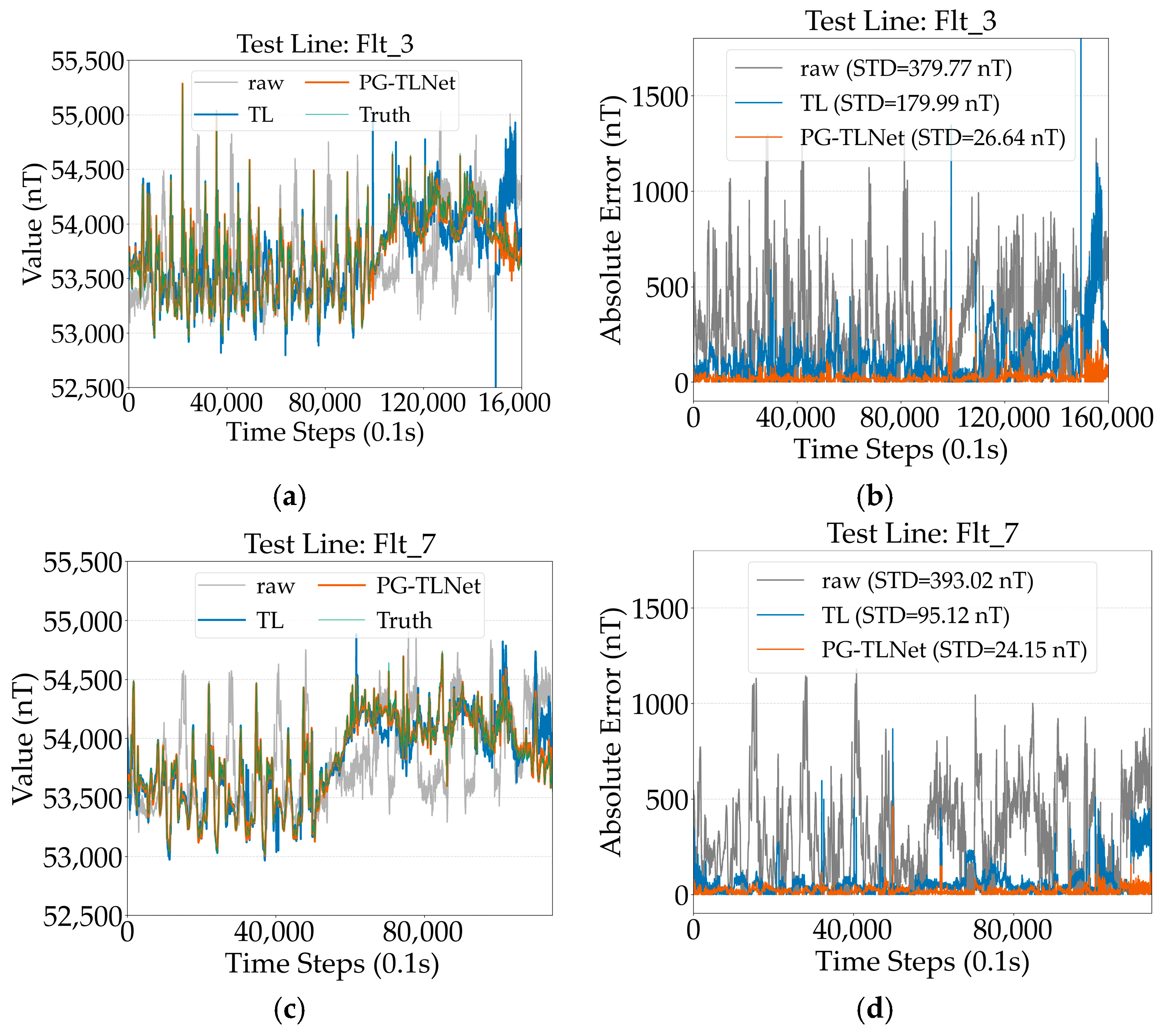
For each test flight, the corresponding compensation results are illustrated in Figure 5. In the figure, the green curve denotes the reference ground truth measured by the low-interference magnetometer Mag_1, the gray curve represents the raw uncompensated measurements from Mag_3, the blue curve corresponds to the compensation result of the conventional Tolles–Lawson (T–L) model, and the orange curve shows the output of the proposed PG-TLNet method. As shown in Figure 5a,c, the PG-TLNet results closely follow the reference signal, exhibiting substantially reduced fluctuations compared with both the raw measurements and the T–L compensated results. In contrast, the T–L model retains noticeable residual oscillations, particularly during long-duration and dynamically varying flight segments. The corresponding absolute error plots in Figure 5b,d further highlight the performance differences among the methods. For Flt_3, PG-TLNet achieves an the standard deviation (STD) of 26.64 nT, representing 85.2% reduction relative to the T–L model (179.99 nT). For the more challenging Flt_7 flight, the STD is further reduced to 24.15 nT, corresponding to a 74.61% improvement over the T–L baseline (95.12 nT). In both test cases, the T–L model exhibits pronounced fluctuations and residual error accumulation over time, which limits its suitability for sustained aeromagnetic compensation under strong interference conditions. In contrast, the proposed PG-TLNet framework maintains consistently low residual levels throughout the entire flight duration, even when evaluated on test flights that are temporally separated from the training data, demonstrating strong stability and generalization capability. Under high-maneuvering conditions, occasional transient error peaks can still be observed in the PG-TLNet results. These peaks are likely induced by rapid variations in the platform’s electromagnetic environment during aggressive maneuvers. Nevertheless, their magnitudes remain tightly bounded and do not lead to cumulative error growth, indicating that the proposed framework preserves robustness under strongly disturbed and highly dynamic operating conditions, which are representative of onboard UAV magnetic sensing and navigation scenarios.

In this study, STD is used as a measure of data error. In addition, the Improvement Ratio (IR), widely adopted by the National Research Council Canada [34], In this study, the standard deviation (STD) of the magnetic error is adopted to quantify the fluctuation level of measurement errors. In addition, the Improvement Ratio (IR), which has been widely used in aeromagnetic compensation studies by the National Research Council of Canada (NRC), is employed as a key performance indicator for evaluating magnetic interference compensation performance. A larger IR indicates more effective suppression of magnetic interference. The IR is defined as

$$\mathrm{I}\mathrm{R}={\displaystyle \frac{{\sigma }_{\mathrm{r}\mathrm{a}\mathrm{w}}}{{\sigma }_{\mathrm{r}\mathrm{e}\mathrm{s}}}}$$

(25)

where ${\sigma }_{\mathrm{r}\mathrm{a}\mathrm{w}}$ and ${\sigma }_{\mathrm{r}\mathrm{e}\mathrm{s}}$ denote the standard deviations of the uncompensated and compensated magnetic errors, respectively.

The magnetic error at time index $i$ is defined as

$$e_i=B_{\mathrm{p}\mathrm{r}\mathrm{e}\mathrm{d},i}-B_{\mathrm{r}\mathrm{e}\mathrm{f},i}$$

(26)

where $B_{\mathrm{p}\mathrm{r}\mathrm{e}\mathrm{d},i}$ represents the measured or compensated magnetic field, and $B_{\mathrm{r}\mathrm{e}\mathrm{f},i}$ denotes the reference magnetic field. The standard deviation of the magnetic error over a flight segment containing $N$ samples is computed as

$$\sigma =\sqrt{{\displaystyle \frac{1}{N}}\sum _{i=1}^N{\left(e_i−\overline{e}\right)}^2}$$

(27)

where $\overline{e}$ is the mean value of the error sequence. Accordingly, the uncompensated error and residual error are defined as $e_{\mathrm{r}\mathrm{a}\mathrm{w}}=B_{\mathrm{u}\mathrm{n}\mathrm{c}\mathrm{o}\mathrm{m}\mathrm{p}\mathrm{e}\mathrm{n}\mathrm{s}\mathrm{a}\mathrm{t}\mathrm{e}\mathrm{d}}-B_{\mathrm{r}\mathrm{e}\mathrm{f}},e_{\mathrm{r}\mathrm{e}\mathrm{s}}=B_{\mathrm{c}\mathrm{o}\mathrm{m}\mathrm{p}\mathrm{e}\mathrm{n}\mathrm{s}\mathrm{a}\mathrm{t}\mathrm{e}\mathrm{d}}-B_{\mathrm{r}\mathrm{e}\mathrm{f}},$ and their corresponding standard deviations are denoted as ${\sigma }_{\mathrm{r}\mathrm{a}\mathrm{w}}$ and ${\sigma }_{\mathrm{r}\mathrm{e}\mathrm{s}}$, respectively. Both quantities are evaluated over the same flight segment after time alignment to ensure a fair comparison. To further investigate the robustness of the proposed PG-TLNet framework under varying maneuvering conditions, the two test flights Flt_3 and Flt_7 were segmented according to their maneuvering states. Compensation performance was evaluated separately for each maneuver segment to analyze the influence of flight dynamics on residual magnetic interference. The corresponding prediction errors of TL model and PG-TLNet model are summarized in

Table 5. TL model and PG-TLNet model prediction errors for each test segment.

Line	${\mathit{\sigma }}_{\mathbf{T}\mathbf{L}}$	${\mathit{\sigma }}_{\mathbf{P}\mathbf{G}\mathbf{T}\mathbf{L}}$	${\mathbf{I}\mathbf{R}}_{\mathbf{T}\mathbf{L}}$	${\mathbf{I}\mathbf{R}}_{\mathbf{P}\mathbf{G}\mathbf{T}\mathbf{L}}$	Line	${\mathit{\sigma }}_{\mathbf{T}\mathbf{L}}$	${\mathit{\sigma }}_{\mathbf{P}\mathbf{G}\mathbf{T}\mathbf{L}}$	${\mathbf{I}\mathbf{R}}_{\mathbf{T}\mathbf{L}}$	${\mathbf{I}\mathbf{R}}_{\mathbf{P}\mathbf{G}\mathbf{T}\mathbf{L}}$
Flt_3	179.99	26.64	2.11	14.26	Flt_7	95.12	24.15	4.13	16.27
Flt_3.01	63.38	17.40	3.48	12.69	Flt_7.01	66.01	18.15	2.88	10.48
Flt_3.02	27.63	5.86	3.59	16.97	Flt_7.02	31.64	26.04	7.19	8.74
Flt_3.03	110.98	20.44	2.63	14.31	Flt_7.03	26.67	17.95	7.02	10.44
Flt_3.04	146.49	49.96	1.21	3.57	Flt_7.04	73.96	20.27	4.60	16.79
Flt_3.05	18.71	5.80	4.36	14.08	Flt_7.05	140.57	22.09	1.13	7.23
Flt_3.06	31.96	6.57	2.11	10.31
Flt_3.07	89.15	23.31	0.67	2.56
Flt_3.08	355.83	44.30	0.61	4.87

.

By correlating the segment information in Table 4 with the quantitative results in Table 5, it is evident that the proposed PG-TLNet consistently outperforms the conventional Tolles–Lawson (TL) model across all test segments. For Flt_3, the TL residual standard deviation varies widely among segments, reaching up to 355.83 nT, whereas PG-TLNet substantially reduces the residual variability across most segments, with many segments achieving residual STD values below 20 nT. The corresponding improvement ratios ${\mathrm{I}\mathrm{R}}_{\mathrm{P}\mathrm{G}\mathrm{T}\mathrm{L}}$ are generally above 10, with particularly strong gains observed in long-duration steady-flight segments. Segments with more complex motion exhibit relatively lower IR values, indicating increased difficulty in compensating highly non-stationary interference; nevertheless, the overall residual standard deviation is reduced from 179.99 nT to 26.64 nT, yielding an average ${\mathrm{I}\mathrm{R}}_{\mathrm{P}\mathrm{G}\mathrm{T}\mathrm{L}}$ of 14.26.

For Flt_7, which features overall higher maneuvering complexity, PG-TLNet demonstrates even more pronounced performance gains. While the TL residuals remain significant, PG-TLNet consistently constrains the compensated residual standard deviation to below 25 nT across all segments, with most ${\mathrm{I}\mathrm{R}}_{\mathrm{P}\mathrm{G}\mathrm{T}\mathrm{L}}$ values typically ranging from about 7 to 17. The combined result shows a reduction from 95.12 nT to 24.15 nT, corresponding to an ${\mathrm{I}\mathrm{R}}_{\mathrm{P}\mathrm{G}\mathrm{T}\mathrm{L}}$ of 16.27. These results confirm that PG-TLNet provides robust and stable magnetic interference suppression across diverse flight conditions, maintaining high compensation effectiveness even under complex and prolonged maneuvers.

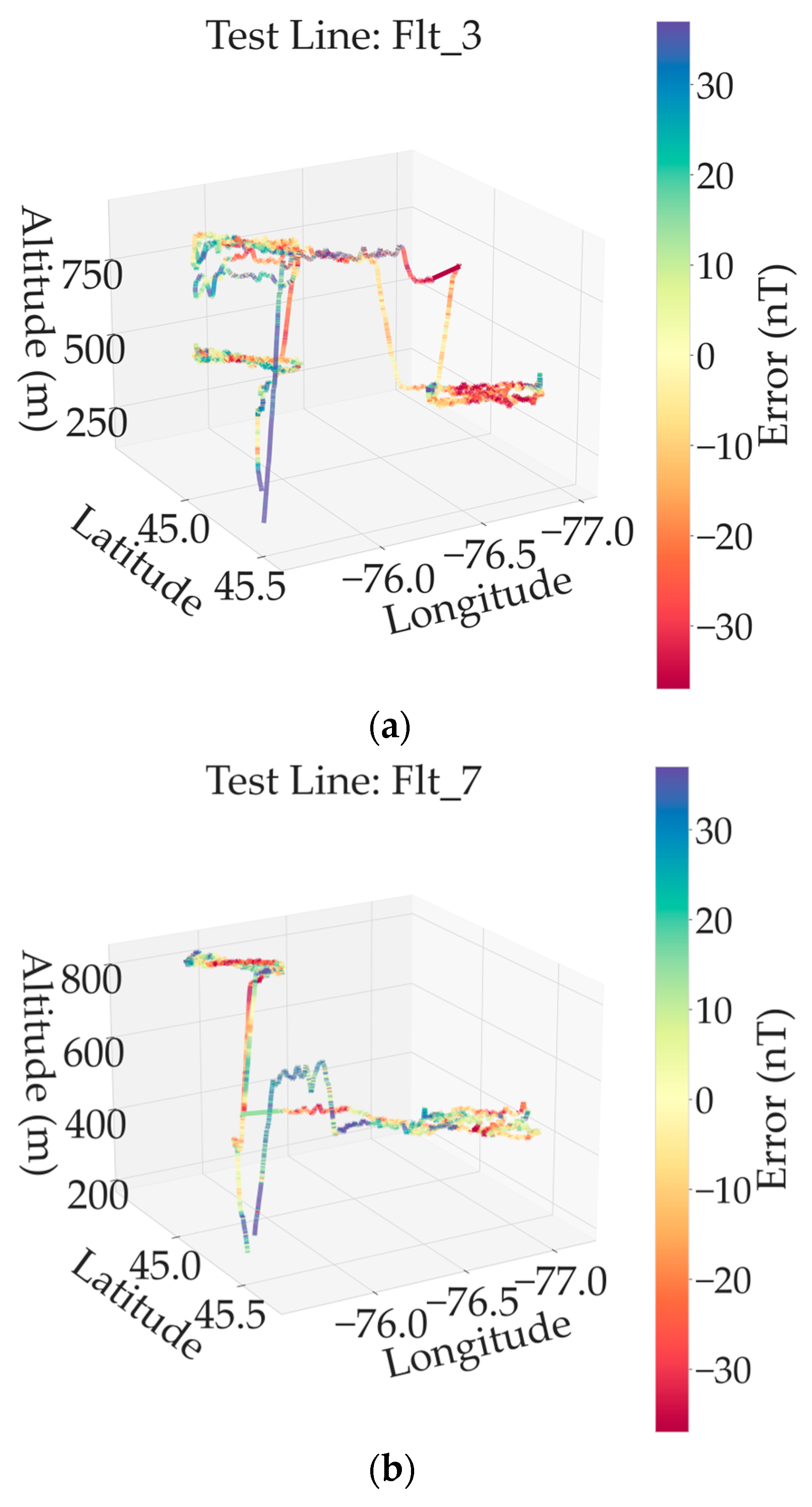
This maneuver-wise evaluation complements the geospatial error analysis presented in Figure 6, enabling a comprehensive assessment of model adaptability from both motion-state and spatial perspectives under strong onboard interference conditions. Figure 6 shows the geospatial distribution of mag3 residual errors predicted by PG-TLNet for Flt_3 and Flt_7. The results indicate that compensation accuracy is primarily influenced by maneuvering complexity rather than altitude variation alone. For smooth or moderately varying flight segments, residuals remain spatially uniform and are generally confined within 25 nT. In segments involving dense turns and rapid heading changes, localized error increases are observed, particularly in the top-view trajectories. Nevertheless, even under these highly dynamic conditions, residuals remain bounded within 30 nT without exhibiting cumulative growth along the flight path. This demonstrates that PG-TLNet maintains stable compensation performance under rapidly varying interference conditions. Across all maneuvering regimes, PG-TLNet consistently outperforms the conventional Tolles–Lawson model, producing smooth, non-accumulative residual distributions. Combined with the STD and IR results in Table 4 and Table 5, these findings confirm that the proposed method achieves robust magnetic interference suppression and provides a reliable magnetic sensing foundation for geomagnetic matching–based navigation.

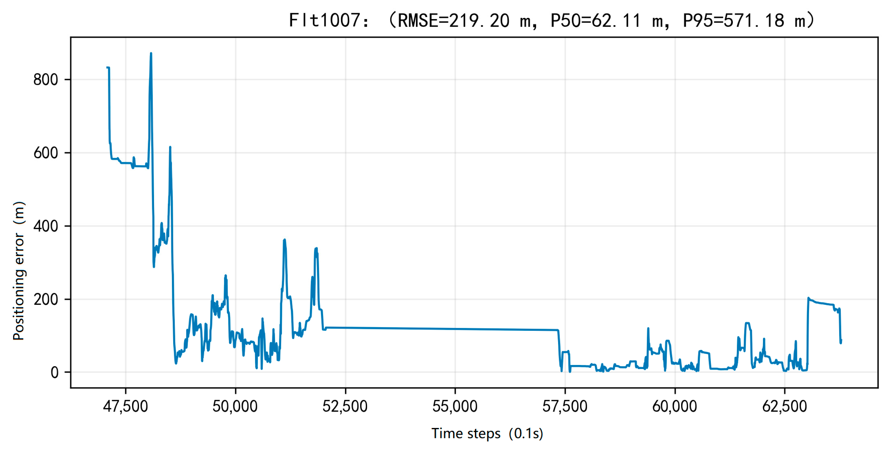
To evaluate the real-time capability of the proposed framework, inference was conducted on two representative test flights, Flt3 (160,000 samples) and Flt7 (114,480 samples). The total processing time for 274,480 samples was 25.72 s, corresponding to an average per-sample latency of approximately 0.094 ms (94 μs). Even at sampling rates exceeding 100 Hz, PG-TLNet occupies less than 1% of the available computation time per sample. Although the current evaluation was conducted in a workstation environment, the low computational complexity and sub-millisecond inference latency suggest that the proposed framework is well-suited for real-time onboard deployment, with substantial computational headroom remaining. An illustrative geomagnetic navigation example based on the compensated magnetic measurements is provided in Appendix A.

$${\mathrm{Latency}}_{\text{per-sample}}={\displaystyle \frac{25.72}{\mathrm{274,480}}}=9.37\times {10}^{-5} \mathrm{s}\approx 94 \mathsf{\mu }\mathrm{s}$$

(28)

4.3. Aeromagnetic Compensation Performance Comparison

To further evaluate the effectiveness of the proposed PG-TLNet framework for aeromagnetic interference compensation, its performance was compared with several representative methods, including the data-driven 1D-CNN-TLNet method [26], the classical backpropagation neural network (BPNN) method [29], and the interference model-guided neural network (IMGNN) method [28]. In addition, the conventional Tolles–Lawson (TL) model was used as a baseline method. The standard deviation (STD) of the uncompensated magnetic measurements (raw data) is also reported for reference.

Table 6. Comparison of aeromagnetic compensation performance for different methods on the test flights Flt_3 and Flt_7.

Model	STD_Flt3 (nT)	STD_Flt7 (nT)
Raw	379.77	393.02
TL	179.99	95.12
PG-TLNet	26.64	24.15
1DCNN-TLNet	27.28	28.29
BPNN	44.49	35.19
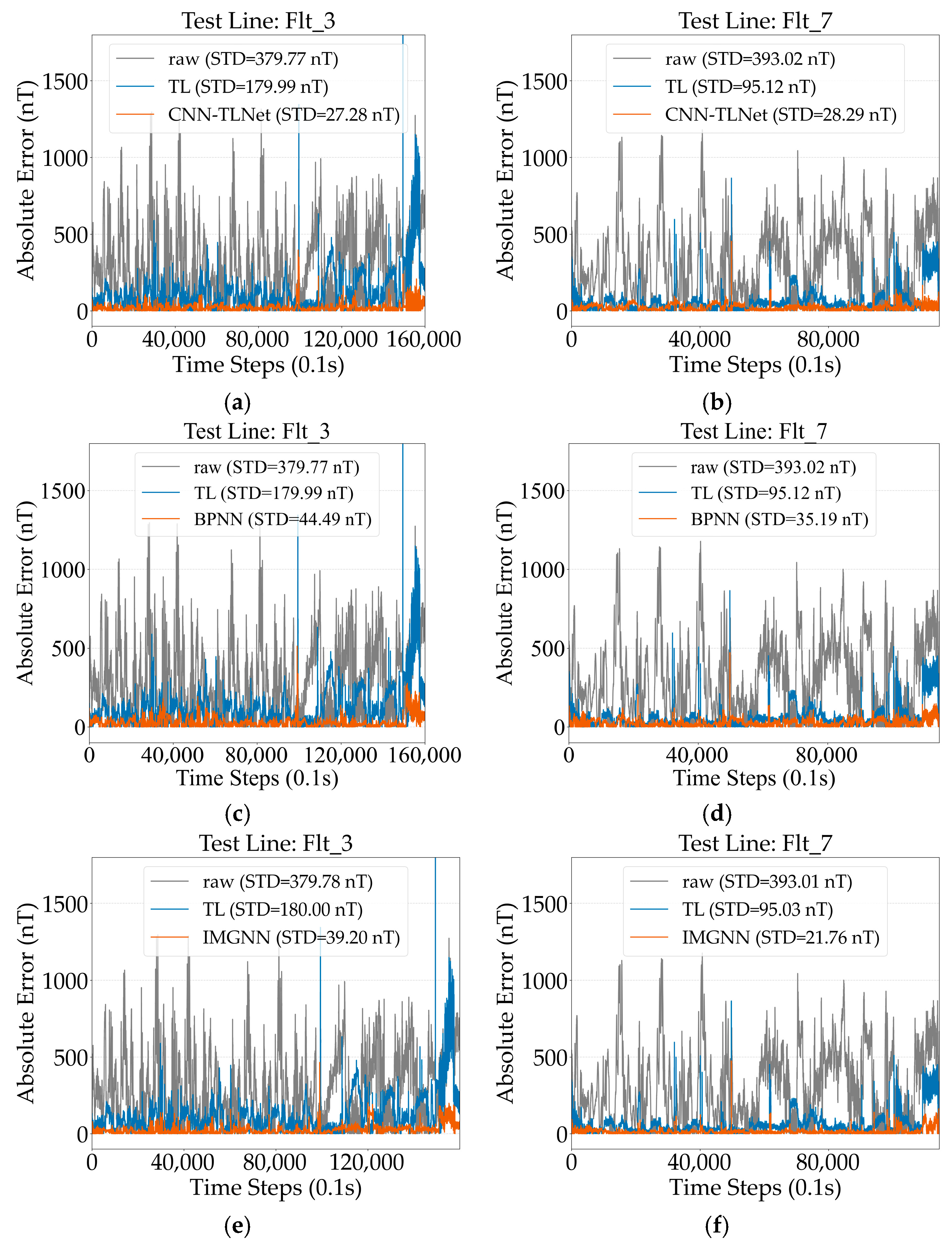
IMGNN	39.20	21.76

presents the absolute error of the magnetic measurements for two representative test flights (Flt_3 and Flt_7) after applying different compensation algorithms. The gray curves correspond to the raw magnetic measurements, while the colored curves represent the compensated results obtained using different methods.

The comparison results presented in Table 6 and Figure 7 reveal several important observations regarding the performance of different aeromagnetic compensation methods. First, the neural-network-based approaches demonstrate significantly better compensation capability than the conventional TL model, indicating that deep learning techniques are effective in modeling complex and nonlinear magnetic interference. In particular, methods based on convolutional neural networks (CNNs) show both strong compensation performance and stable results across different flight conditions. Both the PG-TLNet and the 1D-CNN-TLNet methods are built upon CNN architectures, and they achieve the lowest residual errors among all evaluated methods.

For the Flt_3 test flight, which involves more aggressive maneuvering and complex dynamic conditions, the raw magnetic measurements exhibit severe fluctuations with an STD of 379.77 nT. The TL model reduces the STD to 179.99 nT, but the residual error remains large due to its inability to capture nonlinear and transient disturbances. The BPNN and IMGNN methods improve the compensation performance to some extent, achieving STDs of 44.49 nT and 39.20 nT, respectively. In contrast, the CNN-based approaches provide substantially better results. The 1D-CNN-TLNet method reduces the STD to 27.28 nT, while the proposed PG-TLNet further decreases it to 26.64 nT. For the Flt_7 test flight, which corresponds to relatively smoother flight conditions, all methods achieve improved performance compared with Flt_3. The TL model reduces the STD from 393.02 nT to 95.12 nT, while the BPNN method achieves 35.19 nT and the IMGNN method further improves the result to 21.76 nT. The CNN-based approaches again demonstrate strong performance, with the 1D-CNN-TLNet and PG-TLNet methods achieving STDs of 28.29 nT and 24.15 nT, respectively.

Another notable observation is the stability of CNN-based compensation methods across different flight conditions. The results of PG-TLNet and 1D-CNN-TLNet remain consistently low for both Flt_3 and Flt_7, whereas the performance of the TL, BPNN, and IMGNN methods varies more significantly between the two flight segments. This indicates that CNN-based models are more robust in handling complex maneuver-induced magnetic interference. Overall, the proposed PG-TLNet framework achieves consistently strong performance across both flight tests. By integrating the physical interpretability of the TL model with a structured three-branch CNN architecture, PG-TLNet effectively captures both linear interference components and complex nonlinear disturbances. This hybrid design enables the model to achieve both high compensation accuracy and stable performance under different flight conditions, demonstrating the advantage of combining physical modeling with deep learning for aeromagnetic interference compensation.

4.4. Cross-Node Consistency Evaluation for Swarm Deployment

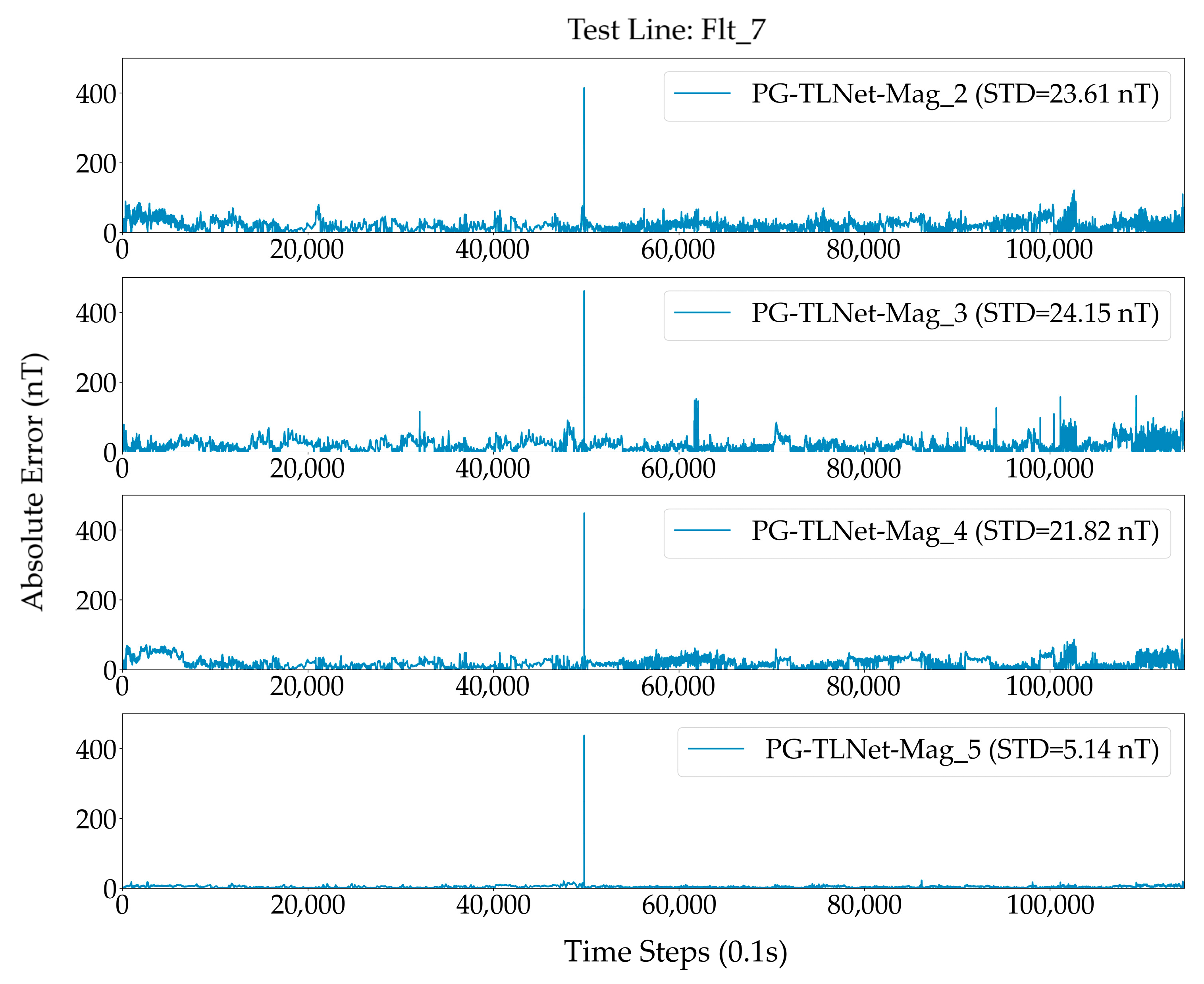
In UAV swarm systems, cooperative geomagnetic navigation requires each UAV node to provide reliable and mutually consistent magnetic measurements. To evaluate the swarm-deployability of PG-TLNet without introducing additional assumptions about inter-vehicle communication, we perform a cross-node consistency analysis by treating each scalar magnetometer channel as an independent sensing node. The dataset contains five optically pumped scalar magnetometers (Mag_1–Mag_5) installed at different platform locations, covering regions with significantly different interference levels. Mag_1 is mounted at a location relatively far from major onboard interference sources and is minimally affected by platform-induced disturbances, and is therefore used as an approximate reference measurement. In contrast, Mag_2, Mag_3, Mag_4, and Mag_5 are installed at near-body locations with varying degrees of interference. For this cross-node evaluation, we focus on the Flt_7 flight line. For each sensing node k ∈ { Mag_2,Mag_3, Mag_4, Mag_5}, we apply the same compensation pipeline and model configuration as used in the main experiments. The compensated output is compared against Mag_1 to quantify both node-to-reference accuracy and node-to-node consistency. Figure 8 visualizes the temporal stability and cross-node consistency of the compensated outputs, illustrates the time-series absolute residual errors of PG-TLNet for Mag_2, Mag_3, Mag_4, and Mag_5 along the Flt_7 line. Despite the presence of sharp transient disturbances and highly dynamic operating segments, the compensated outputs of all nodes remain stable and bounded.

Extending the evaluation to Mag_2, Mag_4, and Mag_5, the results summarized in

Table 7. Cross-node aeromagnetic compensation performance for swarm-oriented evaluation.

Node	${\mathit{\sigma }}_{\mathbf{r}\mathbf{a}\mathbf{w}}$	${\mathit{\sigma }}_{\mathbf{P}\mathbf{G}\mathbf{T}\mathbf{L}}$	${\mathbf{I}\mathbf{R}}_{\mathbf{P}\mathbf{G}\mathbf{T}\mathbf{L}}$	Line
Mag_3	393.02	24.15	16.27	Flt_7
Mag_2	385.40	23.61	17.426	Flt_7
Mag_4	211.50	21.82	9.695	Flt_7
Mag_5	99.26	5.14	19.347	Flt_7

show that PG-TLNet consistently reduces the node-to-reference residuals across all sensing nodes, the wide spread of ${\sigma }_{\mathrm{r}\mathrm{a}\mathrm{w}}$ confirms the heterogeneous interference conditions across sensing nodes. For strongly interfered sensors, the residual error standard deviations are concentrated in the 20–30 nT range, while for weakly interfered sensors they are below 10 nT. Compared with the raw measurements, the dispersion among node outputs is significantly reduced, indicating enhanced cross-node consistency. For the worst-case sensor Mag_3, the main results already demonstrate that PG-TLNet substantially improves compensation performance under severe interference conditions. In addition, the pairwise differences among compensated node outputs exhibit markedly lower dispersion than those obtained using the uncompensated data, further confirming improved cross-node measurement consistency.

Overall, these results demonstrate that PG-TLNet not only provides robust single-node interference suppression, but also effectively homogenizes magnetic measurement quality across heterogeneous sensing nodes. By mitigating large node-to-node discrepancies induced by platform-dependent interference, the proposed framework establishes a reliable and consistent magnetic sensing foundation for cooperative geomagnetic navigation and localization in UAV swarm systems, particularly under GNSS-denied conditions.

When transferring the model to another UAV platform, the TL coefficients can be recalibrated using a short calibration flight, while the CNN parameters can be fine-tuned using a small amount of platform-specific data. Because the CNN primarily learns generic nonlinear interference patterns rather than platform-specific linear components, the required retraining effort is significantly reduced. In addition, the multi-branch feature structure of PG-TLNet separates magnetic, electrical, and kinematic information, which further improves the adaptability of the model to heterogeneous UAV platforms with different electrical architectures and sensor layouts. Therefore, the proposed framework provides a practical and scalable solution for aeromagnetic interference compensation in heterogeneous UAV swarm systems.

4.5. Ablation Study

4.5.1. Feature-Source Ablation

To further analyze the influence of different auxiliary feature sources, a feature-source ablation study was conducted using a two-branch CNN architecture. In all configurations, the first branch processes magnetic sensor data, while the second branch incorporates either electrical features or maneuver-related features, enabling a clear assessment of their individual contributions.

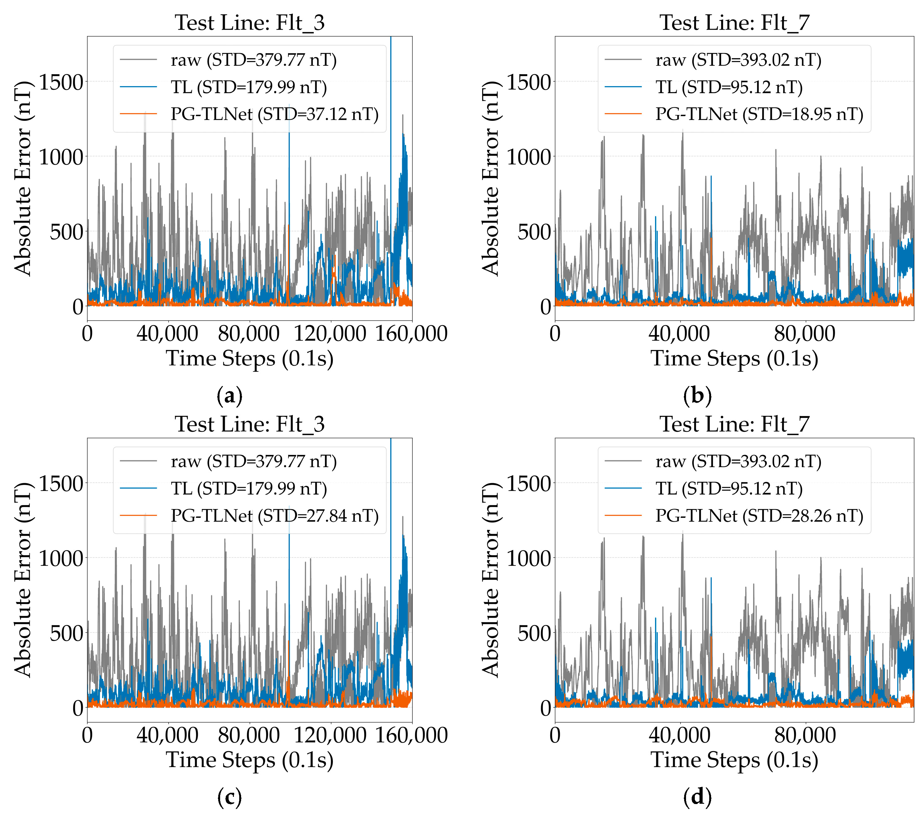
The results using only electrical features (cur_flap, cur_heat, cur_ac_hi, cur_ac_lo, cur_strb, cur_tank, vol_bat_2, vol_block) are shown in Figure 9a,b. For Flt_3, the residual errors remain relatively large and exhibit noticeable fluctuations. This degradation is mainly attributed to the more aggressive maneuvering in Flt_3, where rapid attitude changes introduce interference components that cannot be sufficiently captured by electrical signals alone. In contrast, Flt_7 shows improved performance under the same configuration, benefiting from its relatively smoother and more stable flight profile. These observations indicate that compensation based solely on electrical features is sensitive to flight dynamics and lacks robustness under high-maneuver conditions. Figure 9c,d present the results obtained using only maneuver-related features (ins_roll, ins_vw, ins_yaw, ins_vn, and ins_pitch). In this case, the residual error curves are noticeably smoother across both test flights, indicating stable compensation behavior. However, the overall error magnitude remains higher than that achieved with electrical features in steady conditions. This suggests that while maneuver features effectively model orientation- and motion-induced interference, they cannot fully account for time-varying electromagnetic disturbances driven by onboard electrical systems.

Taken together, these results demonstrate that electrical and maneuver features capture distinct and complementary interference mechanisms. Electrical features are effective in modeling current-induced disturbances under relatively stable motion, whereas maneuver features provide robustness against attitude-related interference but lack sensitivity to electrical load variations. Relying on either feature source alone therefore leads to suboptimal compensation performance. This analysis further justifies the design choice of jointly incorporating both electrical and maneuver information in the proposed PG-TLNet framework, enabling more accurate and robust aeromagnetic compensation under strong interference and highly dynamic flight conditions.

4.5.2. Network Depth Ablation

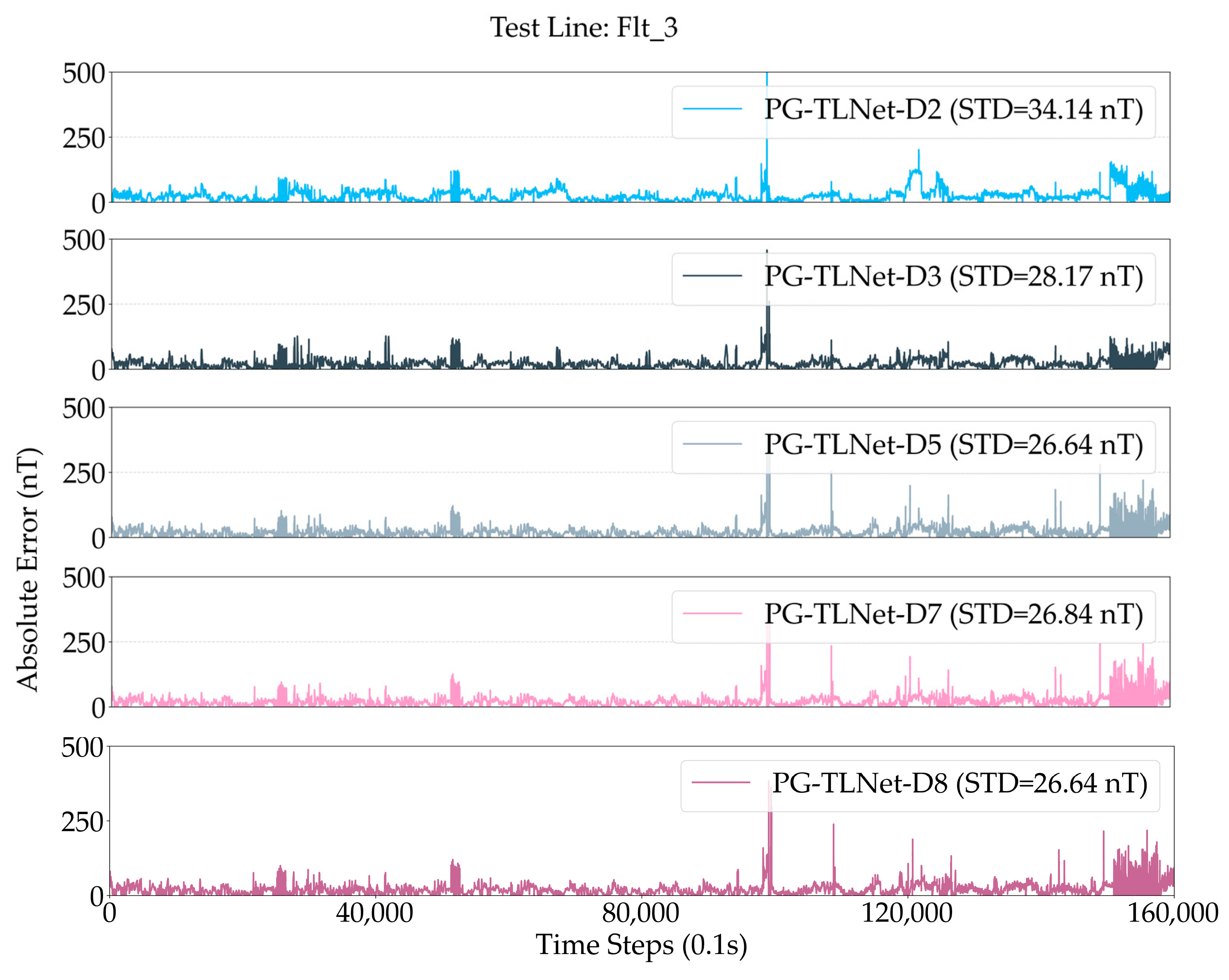
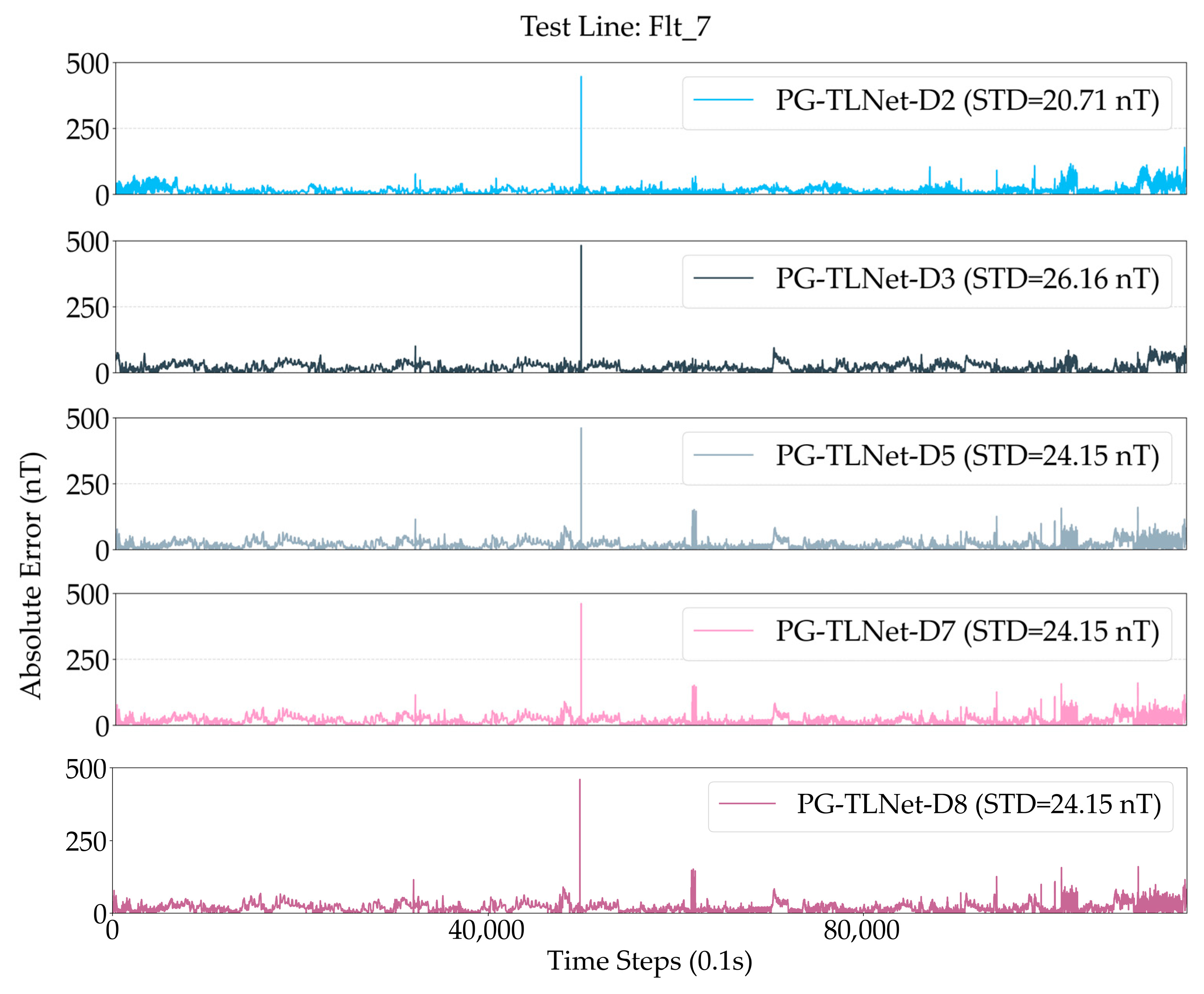
To investigate the influence of network depth on compensation performance, a network depth ablation study was conducted using the proposed PG-TLNet framework. Five configurations with different numbers of convolutional layers (2, 3, 5, 7, and 8 layers) were evaluated while keeping the input features and training strategy unchanged. Figure 10 and Figure 11 present the absolute error results for Flt_3 and Flt_7, respectively.

As shown in Figure 10, increasing the network depth from 2 to 5 layers leads to a clear reduction in residual dispersion for the highly maneuvering Flt_3 flight. Shallow networks (34.14 nT at 2 layers and 28.17 nT at 3 layers) exhibit larger fluctuations and occasional error peaks, indicating insufficient representational capacity to model complex interference dynamics. In contrast, networks with 5 layers achieve substantially lower and more stable error distributions. Further increasing the depth to 7 or 8 layers yields only marginal improvements in STD (26.84 nT at 7 layers and 26.64 nT at 8 layers), suggesting diminishing returns.

A similar trend is observed in Figure 11 for the relatively smoother Flt_7 flight. While deeper networks consistently reduce residual errors compared with shallow ones, the STD stabilizes once the depth reaches five layers. Beyond this point, additional layers do not provide noticeable performance gains, despite increased model complexity. Overall, these results indicate that a five-layer architecture (24.15 nT) is sufficient to capture the dominant nonlinear interference characteristics under both dynamic and steady flight conditions. Considering the rapidly increasing computational cost associated with deeper networks, the PG-TLNet adopts a three-branch, five-layer CNN as a balanced design that achieves robust compensation performance while remaining suitable for real-time onboard UAV applications.

5. Conclusions

This study proposes PG-TLNet, a physics-guided aeromagnetic interference compensation framework designed for high-precision magnetic sensing under strong onboard interference conditions. By tightly integrating an extended Tolles–Lawson (T–L) linear regression model with a lightweight multi-branch convolutional neural network, the proposed approach balances physical interpretability with nonlinear modeling capability. Extensive flight experiments using multiple scalar magnetometers demonstrate that PG-TLNet consistently outperforms the conventional Tolles–Lawson (T–L) model and neural-network-based compensation methods under highly dynamic flight conditions. The proposed method reduces residual magnetic interference from hundreds of nanotesla to the 20–30 nT level, even under interference amplitudes approaching 1000 nT. In addition, the framework improves measurement consistency across sensing nodes, which is beneficial for multi-sensor magnetic measurement scenarios. The results further show that the proposed framework operates in real time, with an average inference latency of approximately 94 μs per sample. This computational efficiency makes the method suitable for practical onboard implementation in aerial platforms operating in complex electromagnetic environments.

Overall, the proposed method provides an effective solution for suppressing platform-generated magnetic interference and establishing a stable magnetic sensing foundation for geomagnetic-field-based navigation and related applications in GNSS-denied environments.

The proposed framework is platform-agnostic and readily deployable across heterogeneous UAV nodes. The achieved compensation accuracy, robustness, and real-time capability indicate that PG-TLNet can effectively support geomagnetic navigation for UAV platforms operating in satellite-denied environments. By ensuring reliable and consistent magnetic measurements at the individual node level, PG-TLNet improves measurement homogeneity across sensing nodes and establishes a critical sensing foundation for cooperative detection and localization in UAV swarm systems. Despite the encouraging results, several limitations should be acknowledged. First, under extreme electrical fault conditions, such as sudden high-current surges or abnormal electromagnetic coupling events, the linear–nonlinear hybrid structure may experience temporary performance degradation due to out-of-distribution signals. Second, in dense swarm operations, potential electromagnetic coupling among closely spaced UAVs may introduce additional interference components that are not explicitly modeled in the present framework. Future work will investigate adaptive domain-shift detection mechanisms and cross-platform transfer strategies to enhance robustness across UAV platforms with radically different electrical architectures. Furthermore, cooperative swarm-level compensation strategies incorporating inter-node communication will be explored.