Predicting Airplane Go-Arounds Using Machine Learning and Open-Source Data †


Abstract
:1. Introduction
2. Pre-Processing and Go-Around Detection
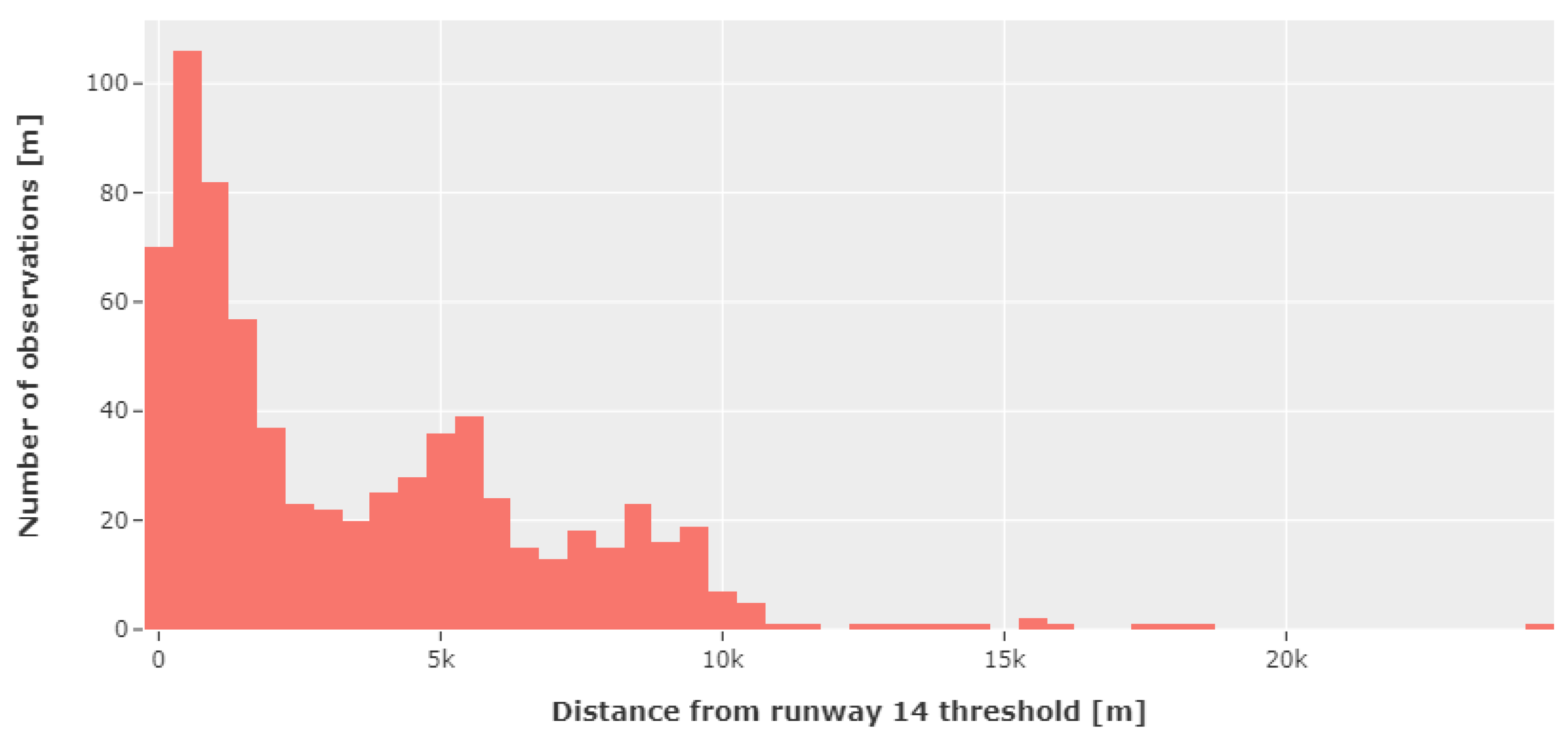
- Landings are defined as trajectories, whose last five observations are (i) within a polygon demarcating Zurich Airport’s limits and (ii) below 600 m above mean sea level.
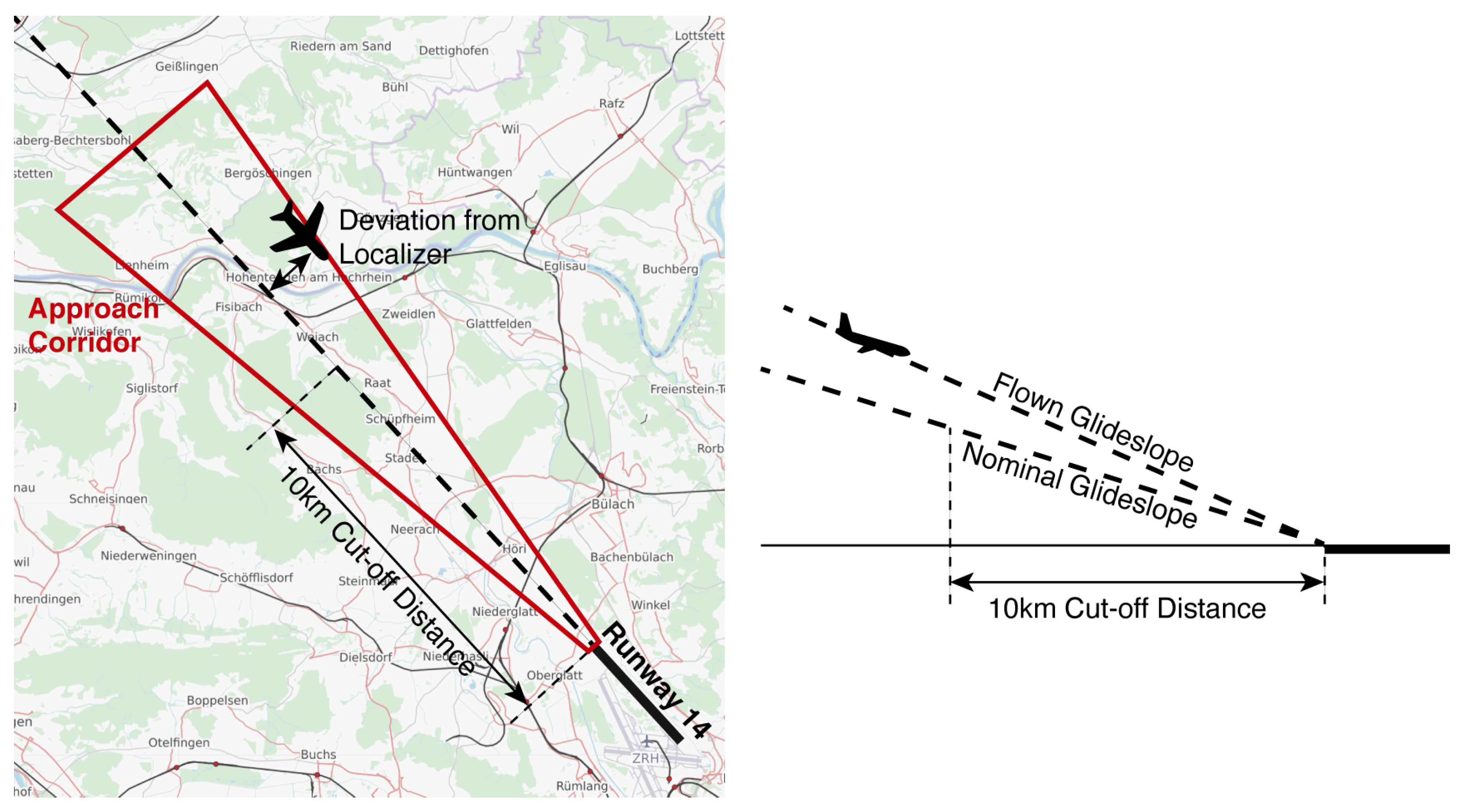
- Landings on runway 14 are defined as a subset of landings observed at Zurich Airport. To be classified as a landing on runway 14, trajectories (i) stay for at least 5 min within a specifically defined approach corridor (see Figure 2) and (ii) have a heading between 126 and 146 degrees during this time.
- GAs are defined as trajectories, which (i) first perform an approach, (ii) leave the approach corridor, and subsequently fly for more than 6 min at an altitude above 800 m above mean sea level. For alternative GA classification methods, the reader is referred to Proud [13].
3. Macroscopic Model: Prediction of GAs in the Next Hour
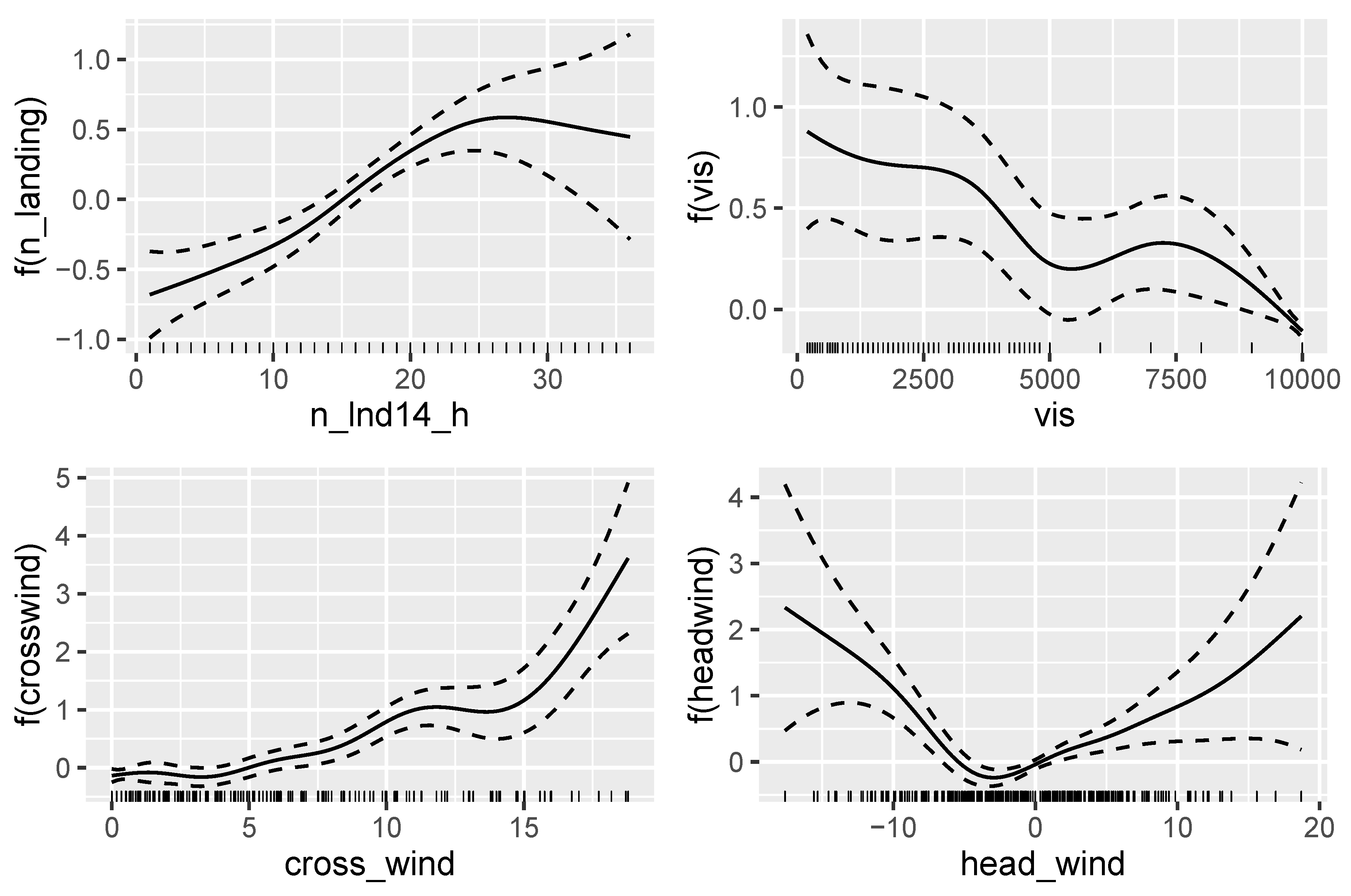
3.1. Modeling
3.2. Results
4. Microscopic Model: Prediction of the GA Probability for an Approaching Aircraft
4.1. Feature Engineering
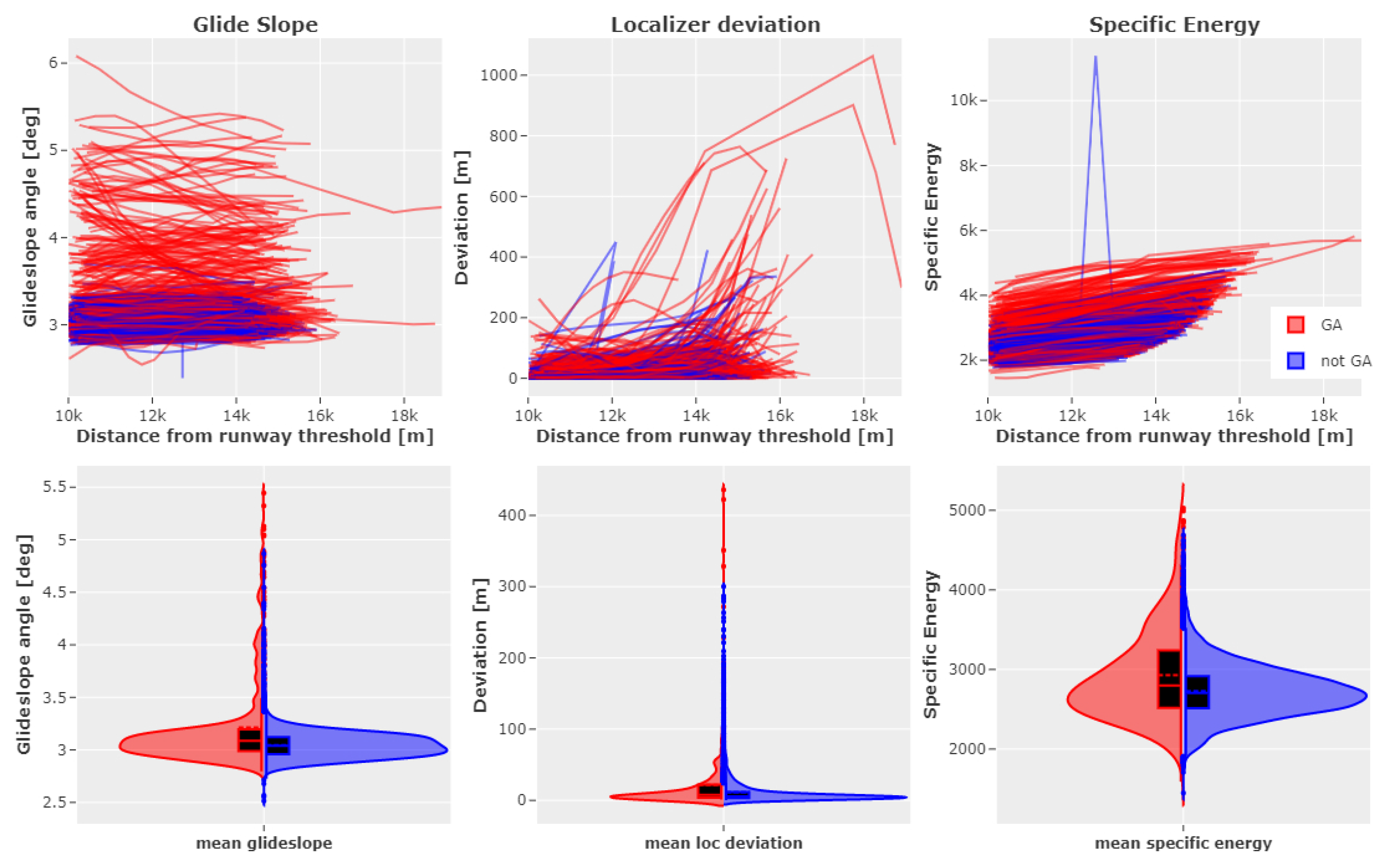
4.1.1. Stability Metrics
4.1.2. Lead–Trail Relationship
4.1.3. Environmental and Aircraft-Related Information
4.2. Modeling
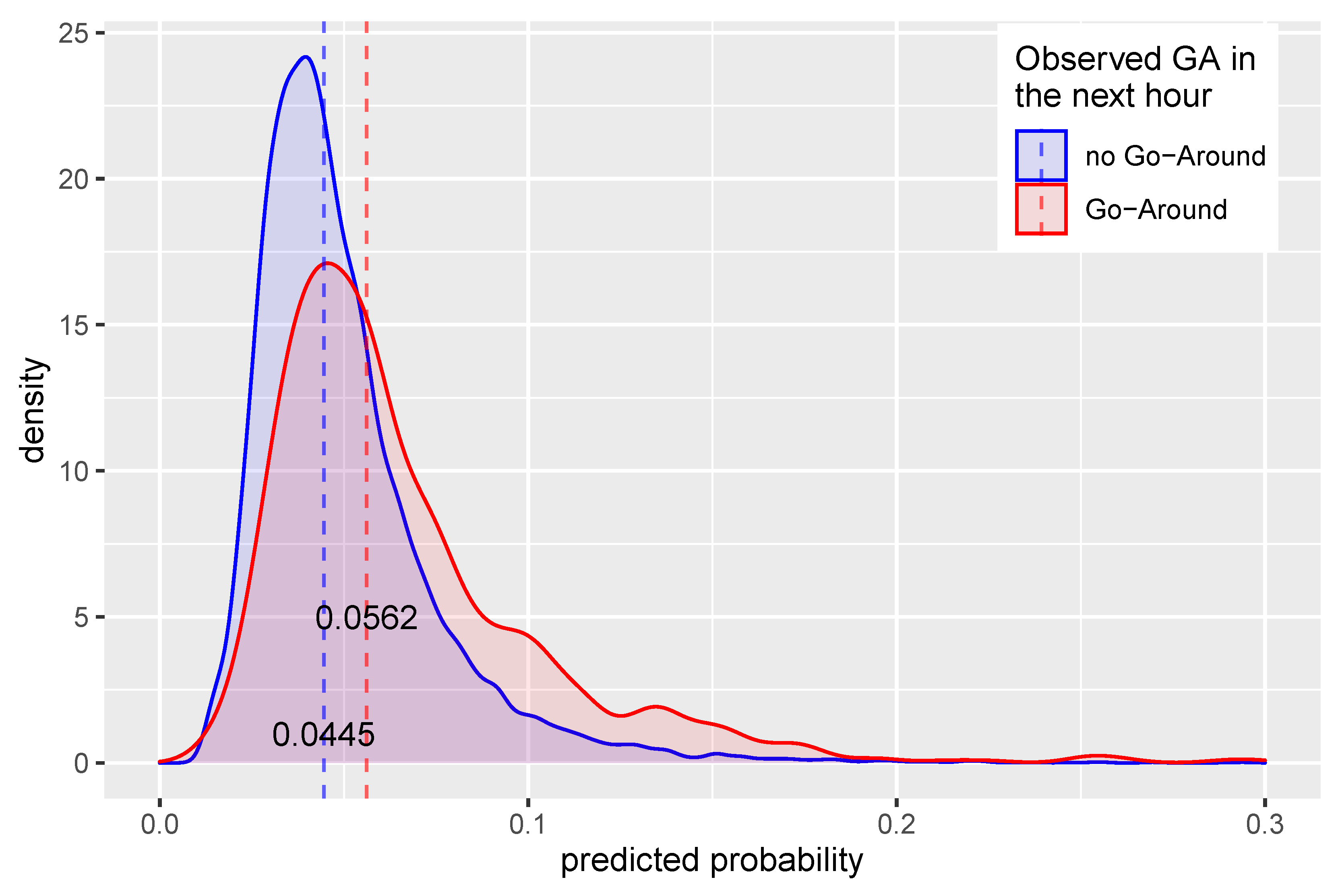
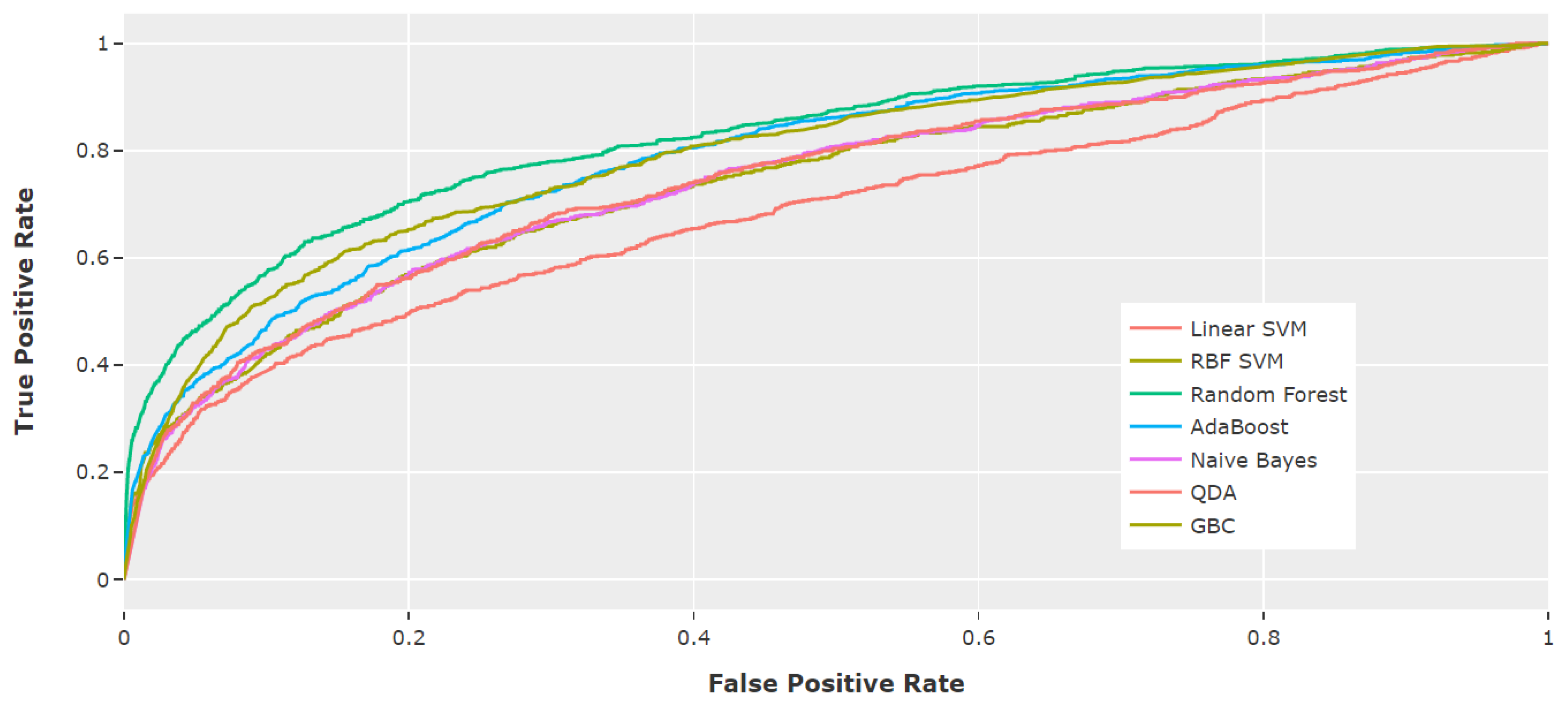
4.3. Results
5. Conclusions
Author Contributions
Funding
Conflicts of Interest
References
- CANSO. Unstable Approaches: Air Traffic Control Considerations. Available online: https://ssd.dhmi.gov.tr/Documents/Unstable%20Approaches-%20Air%20Traffic%20Control%20Considerations.pdf (accessed on 30 October 2020).
- Coker, M. Why and When to Perform a Go-Around Maneuver. Boeing Edge 2014, 2014, 5–11. [Google Scholar]
- Gluck, J.; Tyagi, A.; Grushin, A.; Miller, D.; Voronin, S.; Nanda, J.; Oza, N. Too Fast, Too Low, and Too Close: Improved Real Time Safety Assurance of the National Airspace Using Long Short Term Memory. AIAA Scitech 2019 Forum 2019. [Google Scholar] [CrossRef]
- Gariel, M.; Spieser, K.; Frazzoli, E. On the Statistics and Predictability of Go-Arounds. arXiv 2011, arXiv:1102.1502. [Google Scholar]
- De Boer, R.J.; Coumou, T.; Hunink, A.; Van Bennekom, T. The Automatic Identification of Unstable Approaches from Flight Data. In Proceedings of the Sixth International Conference on Research in Air Transportation (ICRAT 2014), Istanbul, Turkey, 26–30 May 2014. [Google Scholar]
- BFU. Schlussbericht des Büros für Flugunfalluntersuchungen; Schlussbericht 1868; Eidg. Departement für Umwelt, Verkehr, Energie und Kommunikation: Bern, Switzerland, 2005. [Google Scholar]
- Marco Rueckert, Searidge Technologies. Artificial Intelligence in ATM. 2017. Available online: https://emerj.com/ai-sector-overviews/artificial-intelligence-for-atms-6-current-applications/ (accessed on 11 October 2020).
- Christian Thurow, Searidge Technologies. Developing and Deploying AI in Risk Adverse Industries. 2017. Available online: https://on-demand.gputechconf.com/gtcdc/2018/pdf/dc8161-developing-and-deploying-ai-in-risk-averse-industries.pdf (accessed on 11 October 2020).
- Schäfer, M.; Strohmeier, M.; Lenders, V.; Martinovic, I.; Wilhelm, M. Bringing up OpenSky: A large-scale ADS-B sensor network for research. In Proceedings of the 13th International Symposium on Information Processing in Sensor Networks IPSN-14, Berlin, Germany, 15–17 April 2014; pp. 83–94. [Google Scholar]
- Savitzky, A.; Golay, M.J.E. Smoothing and Differentiation of Data by Simplified Least Squares Procedures. Anal. Chem. 1964, 36, 1627–1639. [Google Scholar] [CrossRef]
- OpenSky Network. Aircraft Database. 2020. Available online: https://opensky-network.org/aircraft-database (accessed on 17 August 2020).
- Iowa State University. ASOS-AWOS-METAR Data Download. 2020. Available online: https://mesonet.agron.iastate.edu/request/download.phtml (accessed on 28 July 2020).
- Proud, S.R. Go-Around Detection Using Crowd-Sourced ADS-B Position Data. Aerospace 2020, 7, 16. [Google Scholar] [CrossRef]
- Hastie, T.; Tibshirani, R. Generalized Additive Models; Chapman & Hall/CRC Monographs on Statistics & Applied Probability, Taylor & Francis: Oxfordshire, UK, 1990. [Google Scholar]
- Wood, S.N. Generalized Additive Models: An Introduction with R, 2nd ed.; Chapman and Hall/CRC texts in statistical Science; Chapman and Hall/CRC: London, UK, 2017. [Google Scholar]
- King, G.; Zeng, L. Logistic Regression in Rare Events Data. Polit. Anal. 2001, 9, 137–163. [Google Scholar] [CrossRef]
- Dai, L.; Liu, Y.; Hansen, M. Modeling Go-around Occurrence. In Proceedings of the Thirteenth USA/Europe Air Traffic Management Research and Development Seminar (ATM2019), Vienna, Austria, 17–21 June 2019. [Google Scholar]
- Chawla, N.V. Data Mining for Imbalanced Datasets: An Overview. In Data Mining and Knowledge Discovery Handbook; Springer: Boston, MA, USA, 2010; pp. 875–886. [Google Scholar]
- Saerens, M.; Latinne, P.; Decaestecker, C. Adjusting the Outputs of a Classifier to New a Priori Probabilities: A Simple Procedure. Neural Comput. 2002, 14, 21–41. [Google Scholar] [CrossRef] [PubMed]
- Wold, S.; Esbensen, K.; Geladi, P. Principal component analysis. Chemom. Intell. Lab. Syst. 1987, 2, 37–52. [Google Scholar] [CrossRef]
- Pedregosa, F.; Varoquaux, G.; Gramfort, A.; Michel, V.; Thirion, B.; Grisel, O.; Blondel, M.; Prettenhofer, P.; Weiss, R.; Dubourg, V.; et al. Scikit-learn: Machine Learning in Python. J. Mach. Learn. Res. 2011, 12, 2825–2830. [Google Scholar]


| Formula Name | Predictor |
|---|---|
| thunderstorm | Binary factor, true if a thunderstorm was observed () |
| acTypeshigh | Number of landings of aircraft types classified as high GA probability in the next hour as a fraction of the total number of landing aircraft () |
| acTypesuk | Number of landings of aircraft with unknown GA probability landing in the next hour as a fraction of the total number of landing aircraft () |
| nhomecarrier | Number of landings of home carriers in the next hour () |
| nlanding | Number of landings in the next hour () |
| vis | Visibility in meters |
| crosswind | Absolute crosswind component in knots |
| headwind | Headwind component in knots; positive indicates headwind, negative indicates tailwind |
| Formula Name | Estimate |
|---|---|
| (Intercept) | −3.2 |
| (thunderstorm)) | 0.95 |
| () | 0.68 |
| () | 0.23 |
| () | 0.013 |
| Formula | Feature |
|---|---|
| Glideslope angle , with aircraft at a height above runway and at a distance from the threshold | |
| Localizer deviation : 2D distance between airplane and centerline | |
| Aircraft specific energy (also known as energy height), with aircraft at a height h, ground speed V, and the gravity constant g [3] |
| t [s] | Number of GAs observed when | per 1000 landings |
|---|---|---|
| 200 | 260 | 3.12 |
| 180 | 229 | 3.47 |
| 160 | 178 | 3.96 |
| 140 | 126 | 5.20 |
| 120 | 78 | 8.99 |
| 100 | 43 | 23.4 |
| 80 | 16 | 82.9 |
| Feature Name | Description |
|---|---|
| mean_glideslope | Standardized mean glideslope |
| mean_loc_deviation | Standardized mean deviation from localizer |
| mean_specific_energy | Standardized mean specific energy |
| min_time_to_leader | Minimum observed time to leader, dummy value if no leader |
| leader_wtc_cat | Wake turbulence category of leading aircraft |
| trailer_wtc_cat | Wake turbulence category of trailing aircraft |
| thunderstorm | Binary factor, true if a thunder storm was observed |
| ga_cat | Typecode category for GA probability |
| is_homecarrier | Binary factor, true if the flight is operated ba a home carrier |
| vis | Standardized visibility in meter |
| crosswind | Standardized crosswind component in knots |
| headwind | Standardized headwind component in knots |
Publisher’s Note: MDPI stays neutral with regard to jurisdictional claims in published maps and institutional affiliations. |
© 2020 by the authors. Licensee MDPI, Basel, Switzerland. This article is an open access article distributed under the terms and conditions of the Creative Commons Attribution (CC BY) license (https://creativecommons.org/licenses/by/4.0/).
Share and Cite
Figuet, B.; Monstein, R.; Waltert, M.; Barry, S. Predicting Airplane Go-Arounds Using Machine Learning and Open-Source Data. Proceedings 2020, 59, 6. https://doi.org/10.3390/proceedings2020059006
Figuet B, Monstein R, Waltert M, Barry S. Predicting Airplane Go-Arounds Using Machine Learning and Open-Source Data. Proceedings. 2020; 59(1):6. https://doi.org/10.3390/proceedings2020059006
Chicago/Turabian StyleFiguet, Benoit, Raphael Monstein, Manuel Waltert, and Steven Barry. 2020. "Predicting Airplane Go-Arounds Using Machine Learning and Open-Source Data" Proceedings 59, no. 1: 6. https://doi.org/10.3390/proceedings2020059006
APA StyleFiguet, B., Monstein, R., Waltert, M., & Barry, S. (2020). Predicting Airplane Go-Arounds Using Machine Learning and Open-Source Data. Proceedings, 59(1), 6. https://doi.org/10.3390/proceedings2020059006