Abstract
Increasing demands on a highly efficient air traffic management system go hand in hand with increasing requirements for predicting the aircraft’s future position. In this context, the airport collaborative decision-making framework provides a standardized approach to improve airport performance by defining operationally important milestones along the aircraft trajectory. In particular, the aircraft landing time is an important milestone, significantly impacting the utilization of limited runway capacities. We compare different machine learning methods to predict the landing time based on broadcast surveillance data of arrival flights at Zurich Airport. Thus, we consider different time horizons (look ahead times) for arrival flights to predict additional sub-milestones for n-hours-out timestamps. The features are extracted from both surveillance data and weather information. Flights are clustered and analyzed using feedforward neural networks and decision tree methods, such as random forests and gradient boosting machines, compared with cross-validation error. The prediction of landing time from entry points with a radius of 45, 100, 150, 200, and 250 nautical miles can attain an MAE and RMSE within 5 min on the test set. As the radius increases, the prediction error will also increase. Our predicted landing times will contribute to appropriate airport performance management.
1. Introduction
The air traffic system is developing more and more in the direction of high-performing and efficiency-driven business, which is additionally confronted with extremely high demands on safety and with a growing awareness of the population of the environmental impact of air traffic. These criteria inevitably lead to a multi-criteria optimization problem with conflicting objective functions. In everyday operations, this optimization problem is additionally subject to stochastic uncertainties [1,2]. This makes it difficult to predict the processes even for short prediction periods. An appropriate prediction of the landing time, for example, will significantly improve the Air Traffic Management (ATM), especially the airport efficiency on the day of operations.
Combining both feature engineering and modeling shows promising results to predict gate and runway arrival times [3], using key features, such as aircraft position and weather variables. On the one hand, the aircraft 4D position is broadcast by the aircraft ADS-B (Automatic Dependent Surveillance-Broadcast) transmitter and provides an excellent input for trajectory prediction (opensky-network.org). On the other hand, local airport weather information (provided by METAR messages [4]) and local operational constraints (e.g., airport capacity) enrich the position dataset with the necessary information.
Decision tree methods, such as random forests [1,5,6], are fast to construct, resistant to irrelevant predictors, capable of including both categorical and numerical predictors, and easy to interpret [7]. Thus, the random forest is an ideal tool for trajectory data mining. Other data-driven methods, such as the Hidden Markov Model (HMM) [8] or generalized linear models [9], can also predict aircraft trajectories. A comparison of data mining methods, including linear regression, decision tree, neural networks, and support vector regression, exhibits that the boosting method, a decision tree, outperforms others when predicting the aircraft arrival time considering the described data availability [2]. In our work, we will start by utilizing the feedforward neural network and decision tree methods, such as random forests and gradient boosting machines, to predict the landing time of aircraft in their position 45 nautical miles away from the airport. This approach will be extended to different time horizons by using the intermediate prediction of support points at 250, 200, 150, and 100 nautical miles around the airport. Features are extracted from both ADS-B data and weather information as predictors. Those features, which are important contributors to landing time prediction, are analyzed in Section 2.3.
2. Data Acquisition
2.1. ADS-B Data
The OpenSky Network provides the ADS-B data of aircraft at Zurich Airport (ICAO: LSZH), and we used a dataset from 5 to 31 October 2019, which we downloaded via the Python traffic library [10]. The following data cleaning was accomplished before modeling.
- An index to indicate observations of the same trajectory is added according to the ICAO call sign and timestamp.
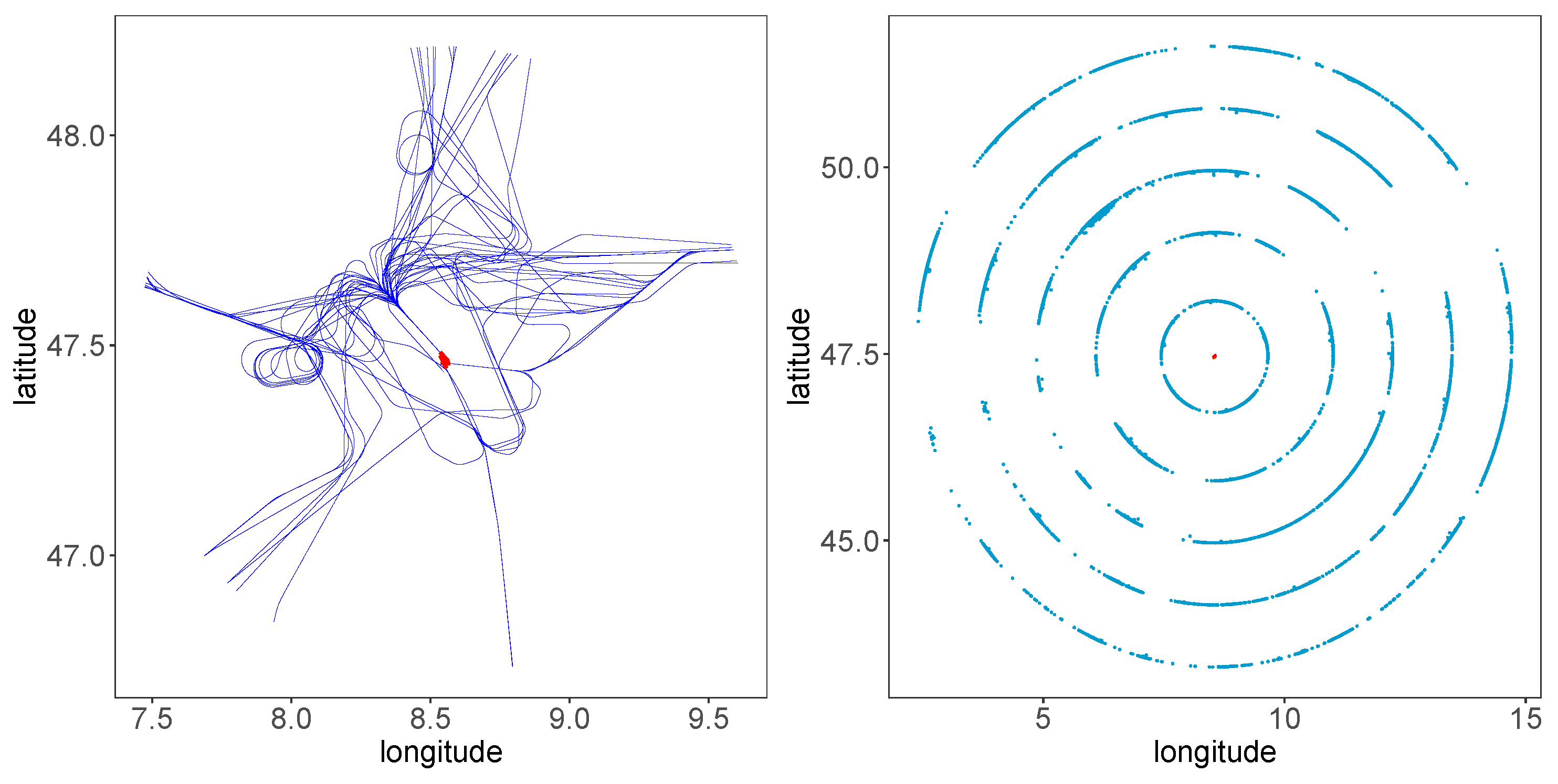
- Trajectories outside the circles of 45, 100, 150, 200, and 250 nautical miles around Zurich Airport are excluded (entry points of these five circles are shown in the right subplot of Figure 1).
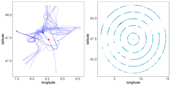 Figure 1. (Left) Sixty sample trajectories approaching Zurich Airport between 5 October 2019 and 31 October 2019, used for landing time prediction in this study. (Right) Entry points of aircraft when 45, 100, 150, 200, and 250 nautical miles away from the runways. The red point in the middle denotes the reference point 47.45 latitude and 8.56 longitude of Zurich Airport.
 - Aircraft passing by but not landing at Zurich Airport are excluded.
- Trajectories with an entry point too close to the runway are excluded as well.
2.2. Weather Data
The second most important input data are weather data obtained by numerically modeled weather output, provided by the National Weather Service of the National Oceanic and Atmospheric Administration (NOAA, www.ncdc.noaa.gov). Therein, the Global Forecast System (GFS) outputs a global weather dataset and provides forecasts with different time horizons. The data include the main atmospheric state parameters, such as temperature T (K), pressure p (Pa), density (kg m), horizontal wind speed to the west u and north v, as well as vertical wind speed w (m s). Every six hours, the data are updated. GFS provides weather data for 64 vertical layers with a lateral resolution of a minimum of degrees. Here, a lateral resolution of degrees is used, which corresponds to ≈ at mid-latitudes.
2.3. Feature Extraction
Both features from ADS-B data and the weather variables are included as predictors. Table 1 provides information about all the predictors. ADS-B data directly provide the following trajectory features: ground speed, track angle, vertical rate, and position variables, such as longitude, latitude, and altitude when entering the circle. Subsequently, the remaining features are calculated from ADS-B data, as described in Table 1.

Table 1.
Summary of features, relevant for the aircraft landing time prediction. GFS, Global Forecast System.
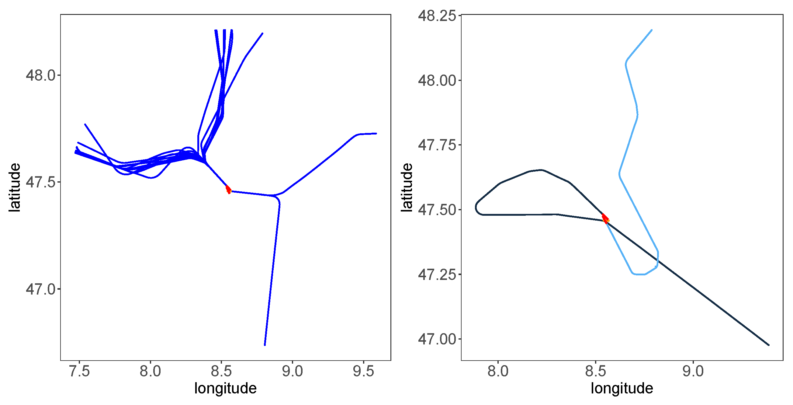
Besides the track angle at the entry point, the track angle when landing on the runway can also be considered. Figure 2 displays two identified patterns: Flights shown in the right subplot have a longer flight time within the 45 NM cycle than the left subplot’s trajectories. The landing time difference can result from more different track angles entering the 45 NM radius circle and landing. The dark blue trajectory in the right subplot changes direction along with its flight, so more distance is traveled, and the angle between the two tracks, the track when entering the circle and the track at the runway, is more than 90 degrees. The difference in the track angle between entering the circle and landing is smaller in the left subplot. The cosine of this track angle between entering and landing tracks is used as a predictor. The track angle at the runway is unknown in practice when predicting when an aircraft is approaching the airport. The angle of the planned runway can substitute this information.

Figure 2.
The difference in the track angle between the entering point on the circle and the landing point. (Left) Trajectories with less landing time; (right) trajectories with more landing time.
To use the direction at the entry point of the circle as a predictor, we clustered the observations using a K-means clustering algorithm. Figure 3 presents an example of entry points at a circle with a 45 NM radius. These entry points can be clustered with the K-means method into seven groups, representing trajectories from seven directions [5]. In the right of Figure 3, the density plot of the landing time of these groups reveals the differences of these trajectories from seven directions.
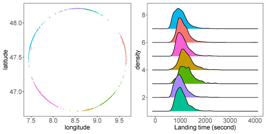
Figure 3.
K-means clustering and landing time by clustering. (Left) Clustered entry points with the radius as 45 NM; (right) density plot of landing time grouped by K-means clusters.
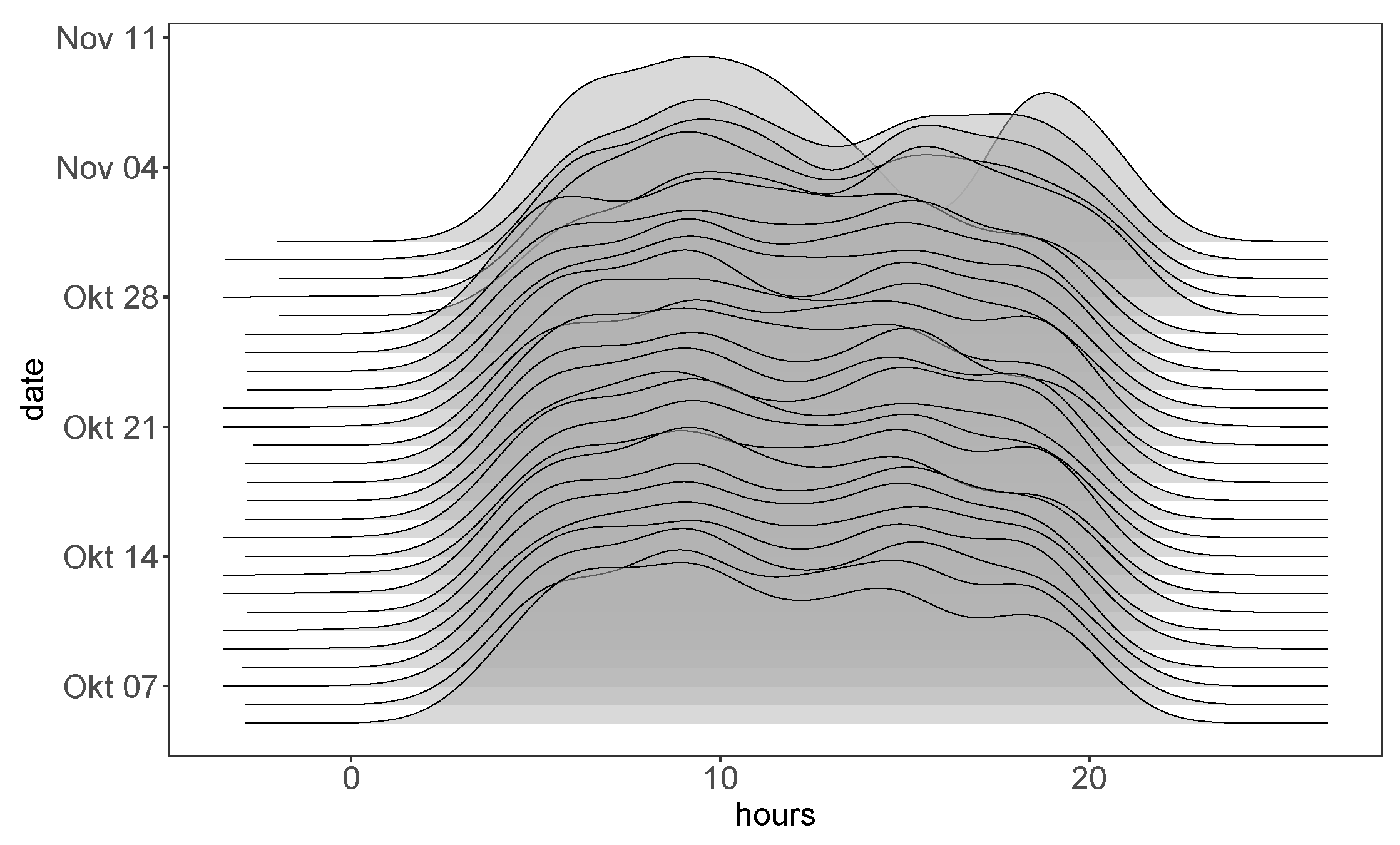
Figure 4 exhibits the traffic density depending on the time with each density layer about the traffic frequency of a day and the height of this plot denoting the number of aircraft entering the circle. The traffic density shown in Figure 4 significantly depends on the time of the day. To extract features regarding the traffic capacity, a time interval, 15 min after this aircraft entering the circle, is considered before or after an aircraft enters the circle. This time interval is then extended to 30 and 60 min before or after an aircraft entering the circle to consider traffic density in the short and long time period. A more precise count of traffic density will not only consider aircraft entering as in Figure 4 but also exclude aircraft landing or departing out of the circle within this time interval. In other words, the number of aircraft in the air and within the circle are counted within a given time interval as features, which is how the features of traffic density in Table 1 are extracted.
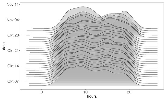
Figure 4.
Traffic density of the day.
Weather variables like temperature, wind speed, and relative humidity also have an impact on landing time. Data from GFS Analysis (www.ncdc.noaa.gov) also represent excellent predictors. Since GFS provides weather updates every 6 h, we use the nearest weather observations temporally at the location 8 degrees longitude and 47 degrees latitude at pressure level 1000 hPa.
2.4. Descriptive Analysis
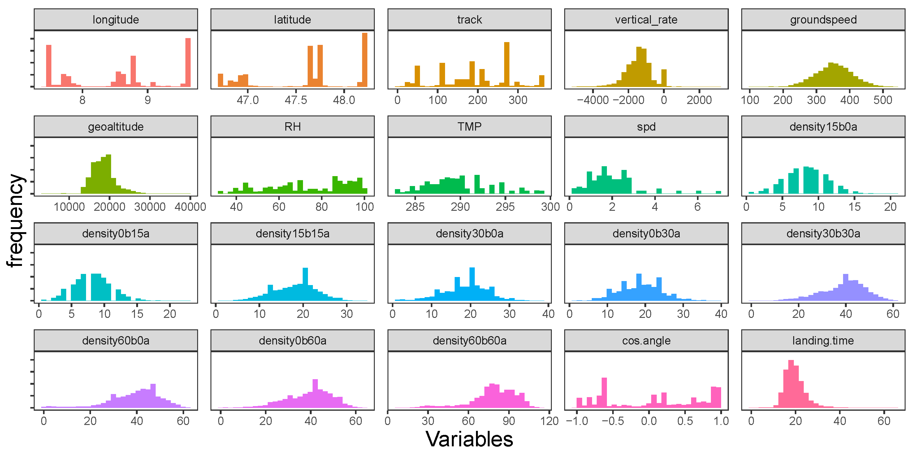
The histogram of numerical features extracted in Table 1 is shown in Figure 5. The landing time can exceed 40 min, as can be seen in the right bottom subplot of Figure 5. Those extreme data are removed in [5,11] to make observations more homogeneous, but not in our work. Features like longitude, latitude, track, relative humidity, temperature, wind speed, and the cosine of the angle between tracks entering and landing do not follow a normal distribution (see Figure 5). Among air traffic density variables, such as time interval increases, the number of aircraft also shifts to the right. In Figure 6, we present Spearman correlations of features and landing time for aircraft entering a circle with a radius of 45 NM. A linear correlation has a parametric assumption of an elliptical distribution, such as a normal distribution [12], which is not the case for most variables in Figure 5. Therefore, the rank correlation measure, Spearman’s Rho, is calculated in Figure 6 instead. Spearman’s Rho (1) is the linear correlation coefficients of the empirical margins, where empirical margin and is the rank of among .
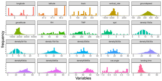
Figure 5.
Histogram of predictors and landing time.
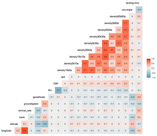
Figure 6.
Spearman correlation between features and landing time.
Hour, weekday, and clustering are categorical features and, therefore, not involved in the correlation matrix in Figure 6. Landing time, in the last column, represents a correlation between most predictors and landing time. Those variables describing traffic densities present a high correlation among themselves.
3. Landing Time Prediction
3.1. Methods and Comparison
After features being extracted, three machine learning methods, the penalized feedforward Neural Network (NN) and the decision tree method, including Gradient Boosting Machines (GBM) and Random Forests (RF), are utilized to predict landing time. A random forest grows a collection of trees by subsetting both observations and variables. Package ranger [13] is applied to fit a random forest method. Gradient boosting machines use a collection of weak learners, modeled by decision trees, to construct a strong prediction model. GBM uses an iterative method to update the model. For each step, the tangent of the cost function is fit by a decision tree and updates the model towards optimal. Package xgboost [14] is applied to fit such a model. A feedforward neural network lets information in the feature space flow through functions, or layers, to map to the target value [15]. We add a penalized parameter to avoid overfitting since the neural network is too flexible and prone to overfitting. We use TensorFlow [16] to construct a feedforward neural network with four hidden layers and norm regularization. To fit hyperparameters like the number of variables in a random forest model and penalty parameters in NN and GBM, we randomly split all observations as the training, validation, and test sets. The test set consists of 20% of all the observations, while the training and validation sets amount to the remaining 80%. The ratios of the training and validation sets are different for the three methods, 4:1 for RF and NN and as a hyperparameter for GBM. Hyperparameters are searched on a grid by the validation set, and the methods are evaluated on the test set. The methods are evaluated using the Root Mean Squared Error (RMSE) and Mean Absolute Error (MAE):
where n is the sample size, is the landing time interval, and is the estimated value in (2) and (3), respectively. Tree methods are better than neural networks. A random forest and a gradient boosting machine have both an MAE and RMSE smaller than 5 min for all radii (see Table 2).

Table 2.
Accuracy evaluation results (RMSE and MAE) of three machine learning methods in order to predict the aircraft landing time. GBM, Gradient Boosting Machine.
3.2. Error with Radius
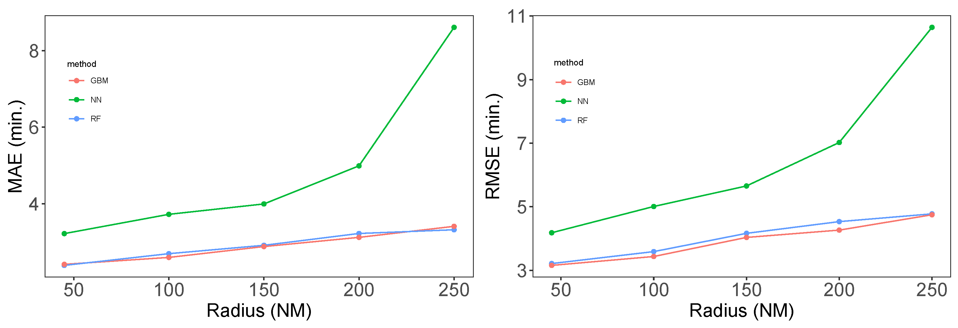
Figure 7 shows line plots of the MAE and RMSE on the test set, depending on the radius. As the radius expands, both the RMSE and MAE grow with the three methods, which was our intuition. While the errors by the tree methods grow slowly, that of NN grows more rapidly. Figure 8 presents a density plot of the error on the test evaluated by the RF method as the radius expands; the density plot expands and becomes flatter, with the error exceeding 30 minutes.
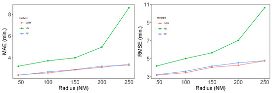
Figure 7.
Line plot of MAE and RMSE depending on the radius by GBM, NN, and RF.

Figure 8.
Density plot of errors on the test set depending on the radius by the RF, GBM, and NN methods.
3.3. Feature Importance
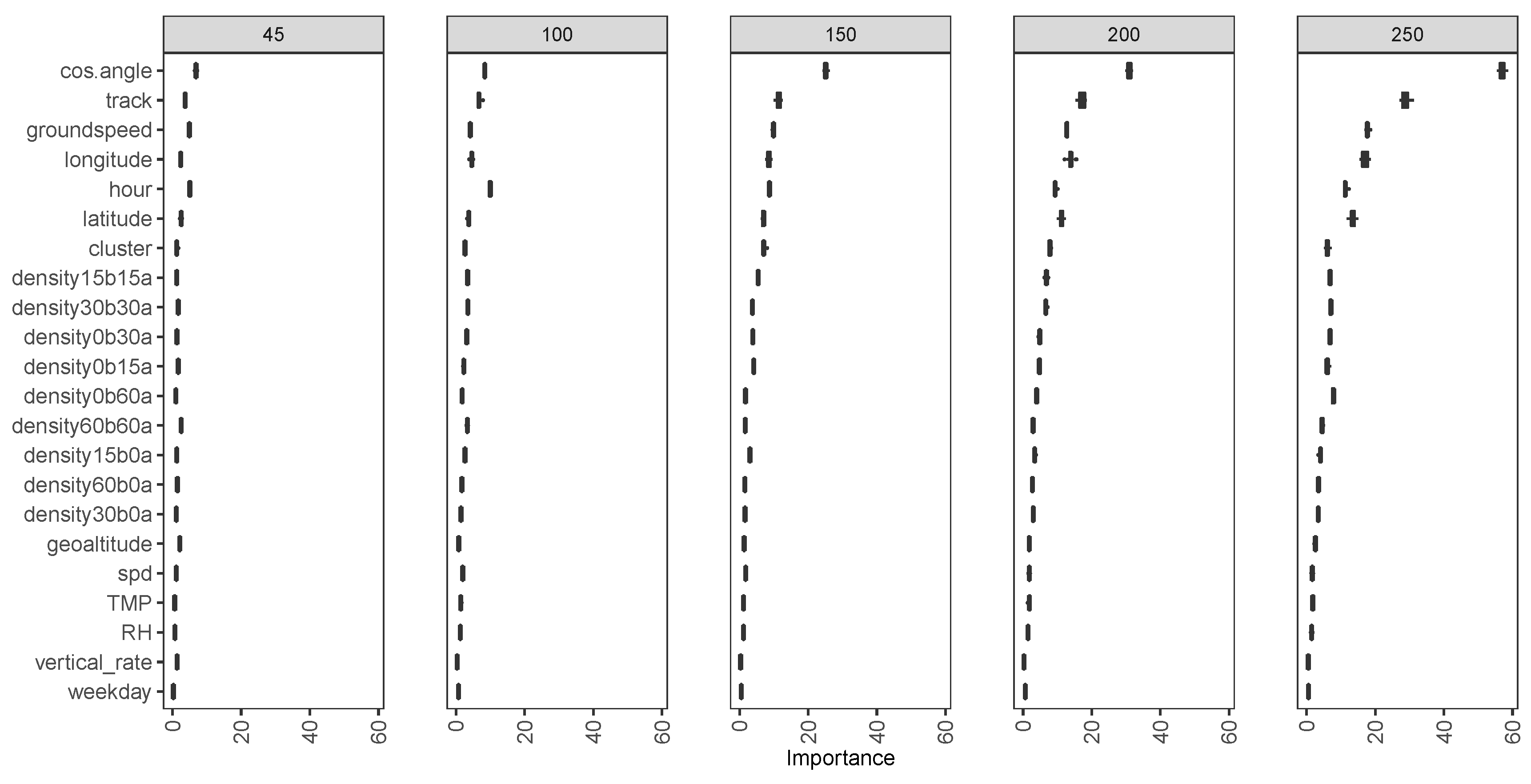
Feature importance identifies those variables that contribute more to the landing time prediction accuracy than others. The importance of features in Figure 9 is measured with random forest, an ensemble of trees with randomness in two ways [17]: (a) each tree is based on a random sample of original data, and (b) each tree considers only a subset of all features. The importance of a feature is measured as the average improvement of accuracy using the Out Of Bag (OOB) error (specifically Mean Squared Error (MSE)) [17] with this feature included. For a tree t, the OOB MSE is calculated by:
where is the number of observations in tree t. Since a random forest permutes features for trees, we have also OOB MSE with feature included and excluded,

Figure 9.
Unconditional Feature importance evaluated by random forest permutation.
If is not an important predictor, the difference should not be comparatively large. The averaged MSE improvement of all trees is used to measure importance. The ranking of feature importance can be derived based on the improved MSE. As the radius increases from 45 NM to 250 NM, the landing time also increases; thus, the scale of MSE also increases. Because of this, the improved MSE can be compared with the same radius, but not for a different radius, in Figure 9. Feature importance results can be sensitive to the number of variables selected in each tree [17,18]. This parameter is set in Section 3.1 to minimize the cost function on the validation set. Random seeds are set as 20 different values for a variation in the boxplot in Figure 9. It shows a variation in importance ranking with different radius, but in general, the cosine of the angle between tracks entering and landing, ground speed, the track angle, longitude, and traffic density are relatively important. Weather variables, such as temperature and relative humidity, are not measured as important since that weather information near the closest observation of GFS analysis data is used.
Strobl et al. [18] recommends using conditional importance, which excludes other variables’ contributions when considering importance for prediction accuracy. However, we are still using unconditional importance for the following reasons: The target for importance analysis is to identify explanatory variables highly related to the landing time, where the unconditional importance would better apply [17]. Moreover, a limited number of variables are included in our model. There is no guarantee to exclude effects from all related variables, even considering conditional importance, making conditional importance results suspicious.
4. Summary
We use data at Zurich airport in October from the OpenSky Network and apply machine learning methods with 22 features extracted from ADS-B data. Decision tree methods, including random forests and gradient boosting machines, can achieve a smaller error than neural networks. The prediction of landing time from entry points at 45, 100, 150, 200, and 250 nautical miles can attain an MAE and RMSE within 5 min on the test set. This result is less striking than in Dhief et al. [5] and Wang et al. [11], who had the MAE and RMSE within one minute. This can result from the fact that no outliers are removed in our work, and only a 25 NM radius was considered in Wang et al. [11].
Some other features can improve the prediction results of the landing time, such as which runway to land, type of aircraft, and region of origin airport. These features can be added to enhance our prediction model. Landing time has a long tail, which makes our estimation error large. The plotting of these trajectory shows a holding pattern. It is worth investigating what triggers such a pattern.
Funding
This paper is part of the project UBIQUITOUS (Using ADS-B big data pattern analysis to improve the quality of multivariate 4D trajectory optimization strategies) and financed by the German Research Foundation (DFG) FR 2440/9-1.
References
- Kern, C.S.; de Medeiros, I.P.; Yoneyama, T. Data-driven aircraft estimated time of arrival prediction. In Proceedings of the 2015 Annual IEEE Systems Conference (SysCon) Proceedings, Vancouver, BC, Canada, 13–16 April 2015; pp. 727–733. [Google Scholar]
- Ayhan, S.; Costas, P.; Samet, H. Predicting estimated time of arrival for commercial flights. In Proceedings of the 24th ACM SIGKDD International Conference on Knowledge Discovery & Data Mining, London, UK, 19–23 August 2018; pp. 33–42. [Google Scholar]
- Takacs, G. Predicting flight arrival times with a multistage model. In Proceedings of the 2014 IEEE International Conference on Big Data, Washington, DC, USA, 27–30 October 2014; pp. 78–84. [Google Scholar]
- Schultz, M.; Lorenz, S.; Schmitz, R.; Delgado, L. Weather impact on airport performance. Aerospace 2018, 5, 109. [Google Scholar] [CrossRef]
- Dhief, I.; Wang, Z.; Liang, M.; Alam, S.; Schultz, M.; Delahaye, D. Predicting Aircraft Landing Time in Extended-TMA using Machine Learning Methods. In Proceedings of the ICRAT 2020 Conference, Tampa, USA, 15 September 2020. [Google Scholar]
- Le, T.H.; Tran, P.N.; Pham, D.T.; Schultz, M.; Alam, S. Short-Term Trajectory Prediction Using Generative Machine Learning Methods. In Proceedings of the ICRAT 2020 Conference, Tampa, USA, 15 September 2020. [Google Scholar]
- Hastie, T.; Tibshirani, R.; Friedman, J. The Elements of Statistical Learning: Data Mining, Inference, and Prediction; Springer Science+Business Media: New York, USA, 2013. [Google Scholar]
- Ayhan, S.; Samet, H. Aircraft trajectory prediction made easy with predictive analytics. In Proceedings of the 22nd ACM SIGKDD International Conference on Knowledge Discovery and Data Mining, San Francisco, CA, USA, 13–17 August 2016; pp. 21–30. [Google Scholar]
- De Leege, A.; van Paassen, M.; Mulder, M. A machine learning approach to trajectory prediction. In Proceedings of the AIAA Guidance, Navigation, and Control (GNC) Conference, Boston, MA, USA, 19–22 August 2013; p. 4782. [Google Scholar]
- Olive, X. Traffic, a toolbox for processing and analysing air traffic data. J. Open Sour. Softw. 2019, 4, 1518. [Google Scholar] [CrossRef]
- Wang, Z.; Liang, M.; Delahaye, D. Automated data-driven prediction on aircraft Estimated Time of Arrival. J. Air Trans. Manag. 2020, 88, 101840. [Google Scholar] [CrossRef]
- Hofert, M.; Kojadinovic, I.; Mächler, M.; Yan, J. Elements of Copula Modeling with R; Springer Nature: Cham, Switzerland, 2019. [Google Scholar]
- Wright, M.N.; Ziegler, A. ranger: A Fast Implementation of Random Forests for High Dimensional Data in C++ and R. J. Stat. Softw. 2017, 77. [Google Scholar] [CrossRef]
- Chen, T.; Guestrin, C. XGBoost: A Scalable Tree Boosting System. In Proceedings of the 22nd ACM SIGKDD International Conference on Knowledge Discovery and Data Mining, San Francisco, CA, USA, 13–17 August 2016; pp. 785–794. [Google Scholar] [CrossRef]
- Goodfellow, I.; Bengio, Y.; Courville, A.; Bengio, Y. Deep Learning; MIT Press: Cambridge, MA, USA, 2016. [Google Scholar]
- Abadi, M.; Agarwal, A.; Barham, P.; Brevdo, E.; Chen, Z.; Citro, C.; Corrado, G.S.; Davis, A.; Dean, J.; Devin, M.; et al. TensorFlow: Large-Scale Machine Learning on Heterogeneous Systems. 2015. Available online: tensorflow.org (accessed on 8 October 2020).
- Grömping, U. Variable importance assessment in regression: Linear regression versus random forest. Am. Stat. 2009, 63, 308–319. [Google Scholar] [CrossRef]
- Strobl, C.; Boulesteix, A.L.; Kneib, T.; Augustin, T.; Zeileis, A. Conditional variable importance for random forests. BMC Bioinform. 2008, 9, 307. [Google Scholar] [CrossRef] [PubMed]
Publisher’s Note: MDPI stays neutral with regard to jurisdictional claims in published maps and institutional affiliations. |
© 2020 by the authors. Licensee MDPI, Basel, Switzerland. This article is an open access article distributed under the terms and conditions of the Creative Commons Attribution (CC BY) license (https://creativecommons.org/licenses/by/4.0/).

