Abstract
Many studies have investigated the forces acting on a football in flight and how these change with the introduction or modification of surface features; however, these rarely give insight into the underlying fluid mechanics causing these changes. In this paper, force balance and tomographic particle image velocimetry (PIV) measurements were taken on a smooth sphere and a real Telstar18 football at a range of airspeeds. This was done under both static and spinning conditions utilizing a lower support through the vertical axis of the ball. It was found that the presence of the seams and texturing on the real ball were enough to cause a change from a reverse Magnus effect on the smooth ball to a conventional Magnus on the real ball in some conditions. The tomographic PIV data showed the traditional horseshoe-shaped wake structure behind the sphere and how this changed with the type of Magnus effect. It was found that the positioning of these vortices compared well with the measured side forces.
1. Introduction
Consistent aerodynamics of association footballs are crucial to enable fair competition in the world’s most popular sport. Many studies have been undertaken to understand how the aerodynamic forces on one football model compare to those on another [,,], or how adding or changing features on a ball can alter the force characteristics [,,,], indicating how sensitive the aerodynamic performance of the ball is to its surface features. Several sources have also investigated what happens to a ball’s aerodynamics when it begins to spin and undergoes either a conventional or a reverse Magnus effect [,,]. These are all useful to quantify the effect that a change will have on the aerodynamic loading (and, hence, flight behaviour) of the ball, but how the surface features on the ball can influence the underlying fluid mechanics is still unclear. This uncertainty means that optimising a football’s aerodynamic performance tends to be based on empirical trends and experience, rather than on an understanding of the fluid mechanics. To begin to develop this understanding, the flow fields must be measured in increasingly quantitative ways.
The flow around a football has been visualized qualitatively using methods such as dust [] or smoke []. It is difficult to extract much quantitative information from these as the flow is unsteady, making repeat measurements difficult. Particle image velocimetry (PIV) is an effective technique to measure the flow due to the large field of view and the good reliability, accuracy and speed []. Two-dimensional planar PIV measurements have been taken on footballs previously [,], but this study utilises tomographic PIV techniques to measure a 3D, three-component flow field in the wake of a smooth sphere and a real football. These are then analysed to identify significant flow features and compare the flow field between the smooth sphere and a real football.
2. Materials and Methods
2.1. Experimental Setup
The tests were all undertaken in the Loughborough University large wind tunnel—a low-speed, open-circuit, closed-jet wind tunnel with a 1.32 × 1.92 m working section. The tunnel can achieve a maximum velocity of 45 m/s and an upper Reynolds number (Re, see Equation (1)) of 7.3 × 10⁵ in the working section based on a football diameter of 0.22 m. In this tunnel, a size 5 football or similar prototype produces a blockage ratio of approximately 1.70%. Thus, the subsequent results have not been corrected for blockage. The clean tunnel turbulence intensity was measured in accordance with Johl et al. [] as 0.15% at 40 m/s. The ball was placed 220 mm above the floor, away from the tunnel boundary layer effects. Further details of the wind tunnel can be found in Johl et al. [].
The balls used were a smooth sphere machined from resin and a real Telstar 18 football filled with expanding foam (see Passmore et al. []. These were mounted to a 20 mm diameter stainless steel shaft, which was connected to a DC motor underneath the tunnel floor. This could spin these balls through a range extending over 500 rpm and were consistent to within ±5 rpm over the duration of a test. See Figure 1a for a setup schematic and Figure 1b for an image of a ball in the tunnel.
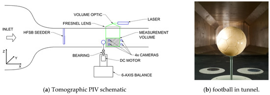
Figure 1.
Wind tunnel setup.
2.2. Balance Measurements
The aerodynamic balance is a high-accuracy, six-axis, under-floor, virtual-centre balance designed for aeronautical and automotive testing. The quoted accuracy for the relevant balance components is ±0.012 N for drag and ±0.021 N for side force. Using an estimate of the expected forces, the resolution is approximately ±0.05% and ±0.50% of the full scale for the drag and lateral components, respectively. Time-averaged force measurements were taken over a period of 120 s; non-dimensional drag (Cd) and lateral force coefficients (Cy) were calculated using Equations (2) and (3):
where: ρ, V, D and μ are the air density, airspeed, ball diameter and dynamic viscosity, respectively; F, A and Vf are the measured force, frontal area and free-stream velocity, respectively.
Balance measurements were captured at spin rates () of 100, 200, 300 and 400 rpm and, at each spin rate, the air speed was increased from 10 to 32 m/s in approximately 3 m/s steps (Re = 1.4 × 10⁵ to 4.5 × 10⁵). This gives a range of spin ratios () between 0.04 and 0.46. The measurements were corrected for the support forces and interference as described by Passmore et al. [].
2.3. Tomographic PIV
Tomographic PIV is a 3D, three-component flow measurement technique. Four cameras were placed in a star formation and are calibrated using a calibration plate to obtain a 3D mapping function. This led to a root-mean-square (RMS) error of below 0.01 px. Seeding particles (helium-filled soap bubbles (HFSB) with an average diameter of 300 μm) were introduced into the flow using a seeding wing at the start of the working section. Laser light was passed through a volume optic and re-collimated using a Fresnel lens to illuminate the target volume. Two images were taken with each camera at a known time separation and corrected using background subtraction techniques and the calibration mapping function; in each test, 1000 image sets were taken at a frequency of 5 Hz.
Using LaVision DaVis v8.4 software, the volume was reconstructed using a FastMART algorithm to calculate where the particles are in 3D voxel space; six passes of this algorithm were used to remove erroneous ghost particles. The reconstructed volume was broken down into decreasing sizes of interrogation window, from 256 voxels down to 96 voxels with 75% overlap; a correlation-based technique was used on these to calculate the 3D velocity vectors. This resulted in a vector density of one vector every 7.7 mm in each dimension. These vectors were post-processed using outlier detection methods to remove spurious vectors and were averaged across the 1000 image sets to produce the flow fields reported. This is a very simplified description of tomographic PIV; for more information about the tomographic PIV setup at Loughborough University, see Pavia et al. [].
3. Results
3.1. Balance Results
Figure 2a shows the drag coefficient against speed for the smooth sphere and Telstar ball in a non-spinning case with the underneath support. These are compared to smooth sphere data from this test, as well as from Achenbach [] and Telstar data by Goff et al. [], all supported from the rear. The underneath mounting is known to affect the balance measurements [] more than the rear support; this is evident here, but it is unavoidable in a spinning test. The rear-supported smooth ball is close to Achenbach’s data. In both setups, the smooth sphere transitions at a higher speed than the Telstar (Re = 2.5 × 10⁵ and 1.5 × 10⁵, respectively, for the underneath support). It is known that the seeding wing also influences the measured forces due to an increase in upstream turbulence; the presented data are all with the wing in place. Figure 2b shows the side force coefficient with the ball spinning at 100 and 300 rpm. In all cases, the smooth sphere has a lower side force than the Telstar ball and exhibits reverse Magnus effects at 100 rpm, which the Telstar does not.
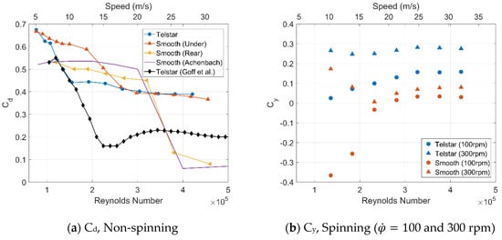
Figure 2.
Time-averaged force coefficients against airspeed.
3.2. Tomographic PIV Results
Figure 3 shows the tomographic PIV results for a range of tests using the smooth sphere. They show a plane that is placed half of the ball radius (r) behind the ball and is coloured according to normalised velocity magnitude (Vmag*). The isosurface is based on the normalised λ2 criterion to identify vortex structures (see Jeong and Hussain [] for definition) and is coloured using normalised streamwise vorticity (ωx*). The interesting features here are the two strong vortices shown by the isosurfaces; these are a counter-rotating pair, shown by the opposite vorticity.
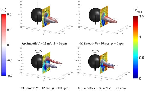
Figure 3.
Tomographic PIV data for a range of conditions with the smooth ball. The isosurface is based on λ2* and coloured by ωx*. The plane is placed at r/2 behind the ball and coloured by Vmag*.
To compare these complex 3D plots in a quantitative way, the normalised Y velocity component (V*) is averaged through the volume. Figure 4 shows this for a range of conditions looking upstream at the rear of the ball ( is from left to right); the streamlines are based on the averaged Y and Z velocity components.
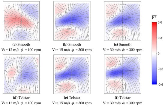
Figure 4.
Averaged normalised V velocity component through the measurement volume for a range of conditions. The streamlines are based on the averaged V and W velocity components.
4. Discussion
The smooth sphere experiences transition at a higher speed than the Telstar ball. There is a difference between the lateral forces experienced by the two balls: At low speed, the sphere and Telstar balls exhibit reverse and conventional Magnus effects, respectively. This is caused by the additional roughness of the Telstar ball’s seams and surface texturing.
The tomographic PIV results show the horseshoe-shaped wake structure typical of the flow over a sphere. This is formed by a counter-rotating vortex pair, as shown in Figure 3 by the two isosurfaces with opposite vorticity values. The shape of this structure is as expected from literature, but does not rotate around the streamwise axis as found previously [,]; it is thought that it is locked to the support required to spin the ball. When spatially averaging the time mean velocity components through the volume (), more negative values are found in those cases with higher Cy. This is expected, as the side force can be considered as a reaction to the change in transverse momentum flux; however, the measurement volume is not large enough to capture the full extent of the wake.
The positions of the vortices move based on the type of Magnus effect experienced; under a conventional Magnus effect (Figure 4b,c,e and f), the vortices move clockwise around the ball; in a case with approximately zero side force (Figure 4d), the vortices are at the bottom of the ball (likely forced by the support), and in a reverse Magnus case (Figure 4a), the vortices move anti-clockwise around the ball. Figure 5 shows the mean position of the two vortices in each of the test cases, coloured by Cy. This position correlates well with the measured Cy value in each case.
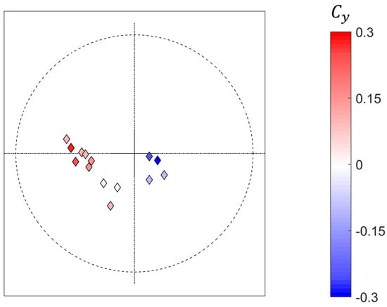
Figure 5.
Mean location of the two vortex cores in each test case, coloured by Cy.
If this understanding between flow structure and aerodynamic forces can be built upon, it may be possible to infer quantitative results from qualitative measurements (e.g., smoke tests). This may help to direct prototype development based on controlling the flow field, rather than on empirical trends.
5. Conclusions
- Balance measurements were captured for a range of airspeeds and spin rates for a smooth sphere and a real Telstar football.
- Tomographic PIV data were captured for the first time on a spinning sphere at points coincident with the balance measurements.
- The roughness on the surface of the Telstar ball triggered a change from reverse to conventional Magnus effect in some conditions compared to the smooth ball (Re < 2.5 × 10⁵ at 100 rpm).
- The tomographic PIV measurements identified the traditional horseshoe-shaped wake structure.
- The two vortices move clockwise around the ball when under a conventional Magnus effect and anti-clockwise in a reverse Magnus effect.
- The angular position of these vortices matched well with the experienced side forces.
Funding
This work was supported by the Engineering and Physical Sciences Research Council.
Acknowledgments
The authors would like to thank Max Varney, Andrew Horsey and Magnus Uruqhart for their assistance with the data acquisition. Many thanks also go to adidas AG for provision of the ball models.
References
- Passmore, M.; Rogers, D.; Tuplin, S.; Harland, A.; Lucas, T.; Holmes, C. The aerodynamic performance of a range of FIFA-approved footballs. Proc. Inst. Mech. Eng. Part P J. Sport. Eng. Technol. 2012, 226, 61–70. [Google Scholar] [CrossRef]
- Goff, J.E.; Hong, S.; Asai, T. Aerodynamic and surface comparisons between Telstar 18 and Brazuca. Proc. Inst. Mech. Eng. Part P J. Sport. Eng. Technol. 2018, 232, 342–348. [Google Scholar] [CrossRef]
- Alam, F.; Chowdhury, H.; Moria, H.; Fuss, F.K. A comparative study of football aerodynamics. Procedia Eng. 2010, 2, 2443–2448. [Google Scholar] [CrossRef][Green Version]
- Rogers, D. A Study of the Relationship Between Surface Features and the In-Flight Performance of Footballs; Loughborough University: Loughborough, UK, 2011. [Google Scholar]
- Hong, S.; Asai, T. Effect of panel shape of soccer ball on its flight characteristics. Sci. Rep. 2014, 4, 5068. [Google Scholar] [CrossRef] [PubMed]
- Naito, K.; Hong, S.; Koido, M.; Nakayama, M.; Sakamoto, K.; Asai, T. Effect of seam characteristics on critical Reynolds number in footballs. Mech. Eng. J. 2018, 5, 17-00369. [Google Scholar] [CrossRef]
- Hong, S.; Goff, J.E.; Asai, T. Effect of a soccer ball’s surface texture on its aerodynamics and trajectory. Proc. Inst. Mech. Eng. Part P J. Sport. Eng. Technol. 2019, 233, 67–74. [Google Scholar] [CrossRef]
- Passmore, M.A.; Tuplin, S.; Spencer, A.; Jones, R. Experimental studies of the aerodynamics of spinning and stationary footballs. Proc. Inst. Mech. Eng. Part C J. Mech. Eng. Sci. 2008, 222, 195–205. [Google Scholar] [CrossRef]
- Passmore, M.A.; Tuplin, S.; Stawski, A. The real-time measurement of football aerodynamic loads under spinning conditions. Proc. Inst. Mech. Eng. Part P J. Sport. Eng. Technol. 2017, 231, 262–274. [Google Scholar] [CrossRef]
- Carré, M.J.; Goodwill, S.R.; Haake, S.J. Understanding the effect of seams on the aerodynamics of an association football. Proc. Inst. Mech. Eng. Part C J. Mech. Eng. Sci. 2005, 219, 657–666. [Google Scholar] [CrossRef]
- Goff, J.E.; Smith, W.H.; Carré, M.J. Football boundary-layer separation via dust experiments. Sport. Eng. 2011, 14, 139–146. [Google Scholar] [CrossRef]
- Asai, T.; Seo, K. Fundamental aerodynamics of the soccer ball. Sport. Eng. 2007, 10, 101–109. [Google Scholar] [CrossRef]
- Adrian, R.J.; Westerweel, J. Particle Image Velocimetry; Cambridge University Press: Cambridge, UK, 2011. [Google Scholar]
- Ruck, S.L.; Spencer, A.; Passmore, M.A. The influence of football surface characteristics on flow separation angle. In Fachtagung ‘Lasermethoden der Strömungsmesstechnik’; Dt. Ges. für Laser-AnemometrieGALA e. V.: Ilmenau, Germany, 2011. [Google Scholar]
- Hong, S.; Asai, T.; Seo, K. Visualization of air flow around soccer ball using a particle image velocimetry. Sci. Rep. 2015, 5, 15108. [Google Scholar] [CrossRef] [PubMed]
- Johl, G.; Passmore, M.; Render, P. Design Methodology and Performance of an Indraft Wind Tunnel. Aeronaut. J. 2004, 108, 465–473. [Google Scholar] [CrossRef]
- Pavia, G.; Varney, M.; Passmore, M.; Almond, M. Three dimensional structure of the unsteady wake of an axisymmetric body. Phys. Fluids 2019, 31, 025113. [Google Scholar] [CrossRef]
- Achenbach, E. Experiments on the flow past spheres at very high Reynolds numbers. J. Fluid Mech. 1972, 54, 565–575. [Google Scholar] [CrossRef]
- Jeong, J.; Hussain, F. On the identification of a vortex. J. Fluid Mech. 1995, 285, 69–94. [Google Scholar] [CrossRef]
- Grandemange, M.; Gohlke, M.; Cadot, O. Statistical axisymmetry of the turbulent sphere wake. Exp. Fluids 2014, 55, 1838. [Google Scholar] [CrossRef]
- Taneda, S. Visual observations of the flow past a sphere at Reynolds numbers between 10000 and 1000000. J. Fluid Mech. 1978, 85, 187–192. [Google Scholar] [CrossRef]
Publisher’s Note: MDPI stays neutral with regard to jurisdictional claims in published maps and institutional affiliations. |
© 2020 by the authors. Licensee MDPI, Basel, Switzerland. This article is an open access article distributed under the terms and conditions of the Creative Commons Attribution (CC BY) license (https://creativecommons.org/licenses/by/4.0/).