Robust Detection of Hidden Material Damages Using Low-Cost External Sensors and Machine Learning ^†

Abstract

Machine learning (ML) techniques are widely used in structural health monitoring (SHM) and non-destructive testing (NDT), but the learning process, the learned models, and the prediction consistency are poorly understood. This work investigates and compares a wide range of ML models and algorithms for the detection of hidden damage in materials monitored using low-cost strain sensors. The investigation is performed by means of a multi-domain simulator imposing a tight coupling of physical and sensor network simulation in the real-time scale. The device under test is approximated by using a mass-spring network and a multi-body physics solver.

1. Introduction

Non-destructive diagnostics and prediction of damage is still a challenge, even in conventional monolithic materials. New materials and hybrid materials, e.g., fiber-metal laminates, are subject to hidden damage without externally visible change of the material. Well-established measuring techniques are ultra-sonic monitoring and computer tomography using X-rays. Both techniques suffer from their high instrumental effort and difficulties in diagnostic robustness. Thus external monitoring of internal damages of such materials and structures with simple and low-cost external sensors like strain gauges under run-time conditions is of high interest. However, there is a significant gap between knowledge and understanding of damage models and the interpretation of sensor data. Machine learning (ML) is a promising method to derive models relating sensor data to damage based on training data, as e.g., shown by Supreet and Harley, who applied artificial neural networks with hidden layers to ultrasonic wave signals to predict structural damage [1]. Although “deep learning” is attractive and en vogue, it commonly requires a high amount of training data and learning time (high computational costs). Thus the investigation of the suitability of and the identification of alternative approaches to deep learning with respect to efficiency is addressed in the present study.

In this work, a multi-domain simulation study is presented comparing and evaluating different ML algorithms and models, i.e., decision trees, e.g., classical C45, and the advanced Interval value Decision tree learner (ICE), artificial neural networks (single and multi-layer perceptrons SLP/MLP), and support vector machines (SVM). A simple plate is used as a device under test (DUT), which is modelled using a simple physical mass-spring network model (MSN), finally simulated (computed) by a multi-body physics engine. The physical computation of the DUT under varying load situations in real-time is directly performed by the simulator combined with an agent-based simulation of signal processing in a distributed sensor network (DSN). Data processing and learning is performed by a collection of agents implementing centralized and distributed agent-based learning [2].

The signals of artificial strain gauge sensors placed on the top side of the DUT surface are computed directly from the MSN and are used to predict hidden damages (holes, inhomogeneities, and impurities) by applying ML to unreliable sensor data. Monte Carlo simulation is used to introduce noise and sensor failures. There are some surprising results concerning robustness and usability of different ML algorithms showing that deep learning is not always suitable.

The simulator (SEJAM2) combining physical and computational simulation can be used as a generic tool for investigation of ML, sensing, sensor design, and distributed data processing. The entire simulation can be controlled by the user via a chat dialogue controlled by an avatar agent. This feature enables the usage of the simulator for educational purposes, too.

There are three major scientific questions addressed in this work: (1) The suitability and accuracy of mass-spring models, especially for modelling of damages in materials and the generation of suitable sensor signals; (2) the suitability of ML for hidden damage detection using noisy and unreliable low-cost sensors; and (3) the comparison of different ML models and algorithms with respect to their prediction accuracy, learning time, and model data size.

2. Modelling and Simulation

Commonly, the finite element method (FEM) is used to simulate the mechanical behavior of engineering structures. This numerical approach for, among others, solving continuum mechanics problems subdivides the component under scrutiny into small, finite elements (hence the name), solves the partial differential equations describing the respective problem numerically for specific points within these sub-domains and assembles the results to a global solution via local approximation functions, which match the functional values obtained for the aforementioned Gauss points and meet certain continuity conditions enforced at transitions between elements. The method as such is accepted and used so widely that it is almost beyond any need for description, much less justification.

However, FEM methods do have disadvantages, which tend not to matter in normal engineering analysis, but suddenly become relevant for the investigations—and applications—behind the present study. Most prominent among these drawbacks is the fact that FEM methods suffer from high computational costs. Typically, the computational effort scales linearly with the number of elements, nodes, and degrees of freedom (DOF) in the case of static problems, as has been demonstrated by Miersch et al. [3].

However, the prerequisite is that sufficient computational resources are available to solve the problem without decomposition of the matrices. If this is not the case, scaling laws will change significantly for the worse. Furthermore, there is a major difference between static and dynamic simulations, which is based on the fact that the latter are usually performed according to a semi-static principle: Either automatically or by the user, an initial time step is selected, which subdivides the time span to be covered into several individual stages, for which static simulations are performed. Even though the length of the time step is typically adjusted during the calculations if stable solutions can be achieved for larger intervals to limit the computational effort, this typically implies an extended effort and thus duration of dynamic as opposed to static calculations. The impact of this general observation on the present study is twofold. First of all, it implies that the FEM method would not be suitable to run on a system that will necessarily have limited computational power as well as energy resources and will thus need to economize on computational effort.

Furthermore, it underlines that an FEM approach, specifically under the aforementioned boundary conditions, is not the optimum choice when real-time solutions are aspired to. For such simulations and evaluation of sensor networks close to the real world, a faster methodology is required, even if this should come at the cost of some levels of accuracy.

There are, however, studies on real-time FEM, but in these, the systems considered tend to be of very low complexity, sometimes with DOF numbers well below 100 [4]. At the same time, alternatives like reduced-order modelling techniques cannot be applied, as they base simplification of the original model on the extraction of special characteristics of the same, while the problem we address in the present work involves damage and thus change of the original system.

For the above reasons, we have chosen a multi-body system approach to represent the material of the structure under study.

In the following sub-section, the basic concepts of multi-body physics are introduced as an alternative method for modelling and simulating mechanical structures on real-time scale.

2.1. Multi-Body Physics

In its most simple case, multi-body simulation deals with kinematic problems: Rigid bodies are assumed to be linked by various types of joints, which differ in their degrees of freedom and thus constrain the respective system’s allowable movements. What is analyzed is motion alone—forces are not accounted for. Multi-body system dynamics (MBSD) add the force component. Now, the rigid bodies can be linked via various types of interactions. These include friction forces but can also simulate materials’ characteristics.

For example, it is possible to connect the rigid bodies via spring- (representing material stiffness), damper- (representing time-dependent, viscous behavior) or friction-type (representing ideal plasticity) elements, or combinations of these. In this sense, viscoelastic properties as seen e.g., in polymers undergoing relaxation are constructed by serial arrangement of spring and damper elements (Maxwell model), whereas creep-like viscoelastic behavior observed e.g. in rubber can be represented by parallel connection of a spring and a friction element (Kelvin-Voigt model).

Naturally, the quality of this type of modelling when describing materials rather than structures does depend on granularity, i.e., on the size of the connected, rigid elements—in fact, in most problems in which multi-body simulations are practically applied, the scale is macroscopic: Examples include vehicle dynamics as well as crash simulations in the automotive area (see [5,6]), covering also bio-mechanical studies [7], or simulations of robotic systems [8].

Several works providing a broad overview of the field both in terms of methods and applications have been published in recent years, e.g., in [5,9,10].

In the current case, though not yet realized in the work we present here, the perspective is towards the microscopic, and to materials rather than structures. For this purpose, we have built up a 3D network of mass elements connected by springs in the manner explained in Section 8. In our approach, this network reflects the behavior of the material, and future evolutions will be increased in resolution.

While this approach may seem unusual for MBSD simulation, it does bear some similarities to notions behind mesh-free simulation methods like smoothed particle hydrodynamics (SPH), discrete element methods (DEM), or material point methods (MPM), which also represent materials on a particle basis and through interactions between these particles [11,12].

Mass-Spring Systems

A mechanical structure is modelled with a Graph St = <M, Sp>, where M is a set of mass nodes with a specific mass m_i, and Sp is a set of spring-damper edges connecting mass nodes.

$$\begin{array}{l}St(P)=\langle M(P),Sp(P)\rangle ,\\ M=\left[\begin{array}{ccc}{m}_1& \cdots & m_j\\ ⋮& \ddots & ⋮\\ m_i& \cdots & m_n\end{array}\right],Sp=\left[\begin{array}{ccc}s{p}_1& \cdots & s{p}_l\\ ⋮& \ddots & ⋮\\ s{p}_k& \cdots & s{p}_m\end{array}\right]\end{array}$$

(1)

Each node m_i has spring connections that are associated with this node pointing to up to seven neighboring nodes (in three dimensions). Details can be found in [13].

The general MSN model graph St(P) is paremeterized by a set of parameters defining the node mass mm_i, the spring stiffness constant sk_j, and optionally a damper constant sd_j. The choice of the parameters, which can be applied to all masses and springs of the network, or individually to domains of nodes and edges, is crucial for the mapping of real, physical material behavior on the physical simulation model described in the next section.

In this work, the node masses and spring constants were chosen to characterize a linear elastic material, typically a purely elastic elastomer.

2.2. Multi-Domain Simulation

• Multi-body physics (MBP) using the CANNON physics engine [14];
• Multi-agent systems and sensor networks using the JAM agent platform.

The CANNON physics engine is a constraint-based multi-body solver that uses an iterative Gauss–Seidel solver to solve constraints and the SPOOK stepper.

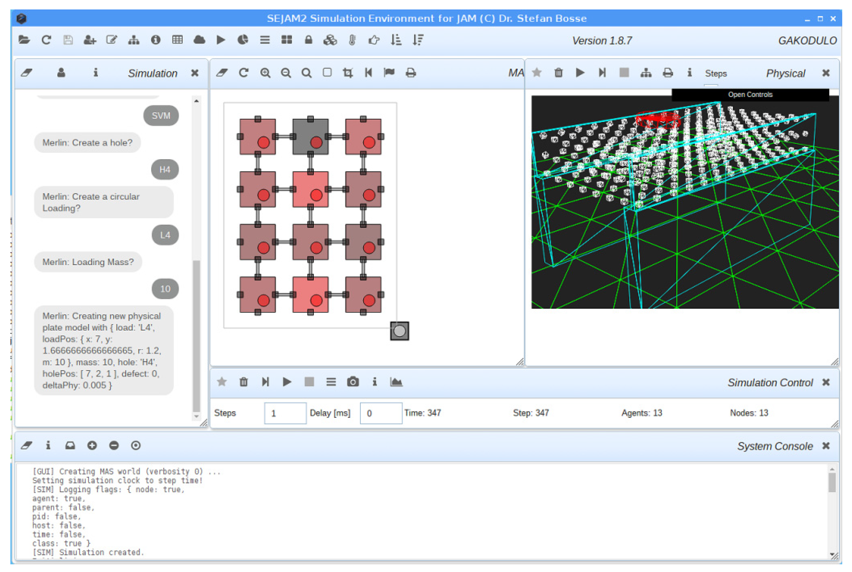
The software architecture of the multi-domain simulator SEJAM2 is shown in Figure 1 and Figure 2. The entire simulator is programmed in JavaScript and processed by node-webkit (embedding the V8 JavaScript high-performance engine). Details can be found in [13,15].

As already stated in the introductory section, the MBP simulation is faster than classical FEM simulation by several orders of magnitude. For example, the simulation of a physical structure consisting of about 330 mass nodes and 2500 springs requires about 50 μs for one update computation of the structure (one physical simulation step, calculation of all mass displacements, forces, and spring forces), using a typical mid-range computer and the JavaScript (JS) V8 engine benchmarking at 22,000k C dhrystones/s and 6600k JS/V8 dhrystones/s, respectively.

Computational complexity and concrete computation times for FEM depend on algorithms, used equation solvers, and the complexity/size of the FEM graph (i.e., the number of elements, basically). In [4], the FEM computation of a simple model using a 1D model with only 11 elements was evaluated for a micro-controller with an Arm Cortex 4 core (at 180MHz clock frequency). The computation time for one static computation (terminating in a stable state) was about one second. Assuming 5000k C-dhrystones/s/GHz for the used machine, this scales to 50ms on the mid-range desktop computer (1000 times slower) considered before; finally, scaled linearly with respect to the number of elements (2500/11), it would require about 10s (or even more). The simulation of the dynamic behavior investigated in this work requires semi-static stepwise FEM simulation accumulating the simulation times for each step. A typical dynamic simulation run requires about 1000 steps. In [3], an investigation of FEM computation times was made with a 3D model showing a more or less linear dependency of the computation time on the number of elements. A structure with about 2000 elements required a computation time of approximately 15 s.

The data processing part is performed by agents executed by the JavaScript Agent Machine (JAM). A physical JAM node supports a world consisting of virtual (logical) nodes (vJAM), which are used to compose the artificial sensor network in the simulation, i.e., each sensor node in the simulation world is represented by a vJAM instance. Agents perform sensor sampling, sensor processing, aggregation, and learning (either centralized by one learning instance or decentralized by multiple learning instances).

2.3. Synthetic Sensors

The physical MBP simulation is primarily used to compute sensor data passed to the digital sensor network. There are basically two classes of sensors and measuring techniques used in SHM and NDT:

• Strain sensors applied to the surface or integrated in the surface layer of a DUT;
• Ultrasonic acoustic sensors and actuators coupled to the surface of the DUT (active measuring technique), or more generally acoustic sensors detecting vibrations of the DUT (passive measuring technique).

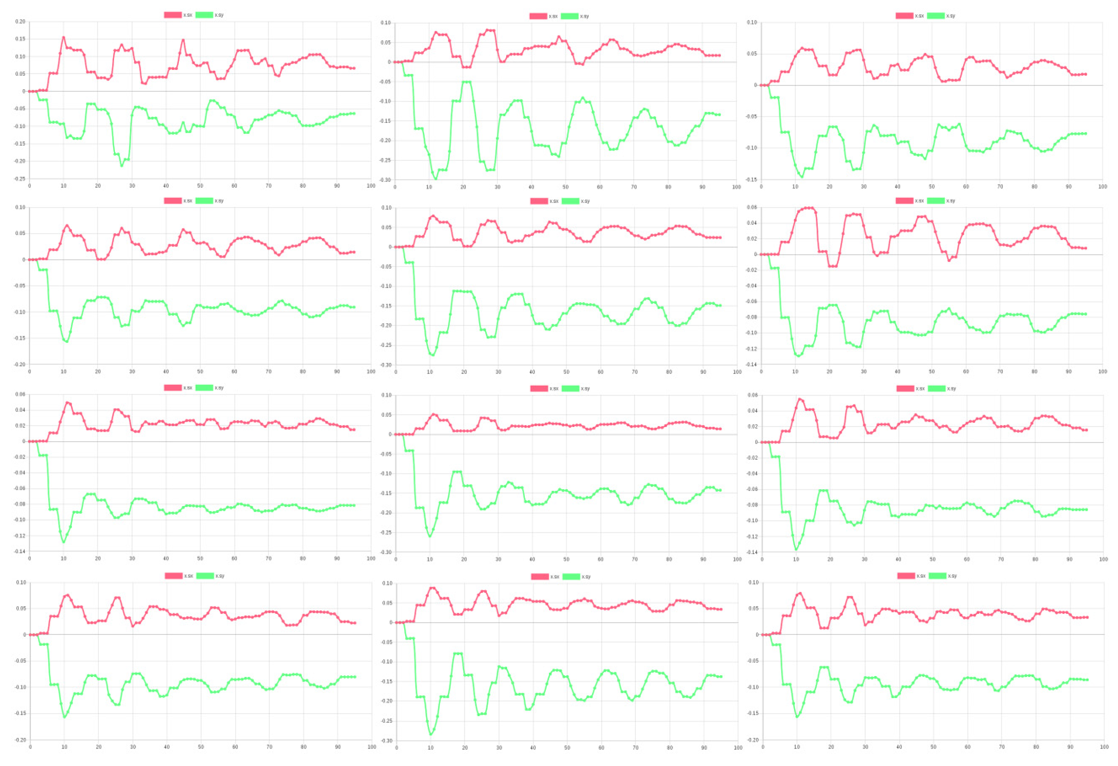
Sensor data of the first class can be directly calculated from the mass-spring network requiring only the distances between mass nodes (available directly from the CANNON engine). A low mass-node density is still sufficient. The second class requires the simulation of the propagation of elastic and acoustic (e.g., lamb) waves in the material, which requires a high density of mass-nodes. Figure 3 shows signals of a spatially distributed strain-gauge sensor network attached to the surface of rectangular plate and getting time-resolved sensor data from the MBP simulation. These plots show the fine-grained and highly time-resolved dynamic behavior of the plate (swinging, starting with an initial and terminating with a final shape caused by gravity).

3. Machine Learning

Machine learning consists basically of three functions:

• The learned model M(x) mapping an input vector x (sensor data) on an output vector y (prediction of system state);
• The training function learn deriving the model function M from (known and labelled) training data;
• The prediction function applying the model function M to unknown (unlabeled) sample data.

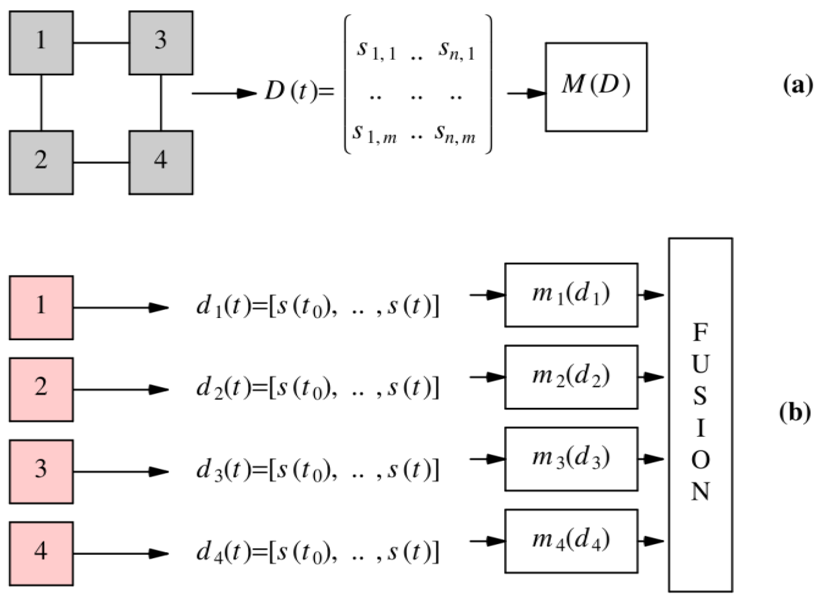
Learning and prediction using sensor data can be performed in two dimensions (see Figure 4):

• Spatial domain. The sensor data D(x, t₀) consists of data from spatially distributed sensors (either the entire sensor network or a sub-domain) sampled at a specific time point t₀ (or accumulated over a time period).
• Time domain. The sensor data are time dependent d(t) and time series of single or a set of sensors are recorded and evaluated.

$$\begin{array}{l}{d}_t(t)=\{s(t_0),s(t_1),s(t_n),..,s(t)\}\hfill \\ D_s(x,t_0)=\left(\begin{array}{ccc}{s}_{1,1}(t_0)& \cdots & s_{n,1}(t_0)\\ ⋮& \ddots & ⋮\\ s_{1,m}(t_0)& \cdots & s_{n,m}(t_0)\end{array}\right)\hfill \\ D_{t-s}(x,t)=\left\{\left(\begin{array}{ccc}{s}_{1,1}(t_0)& \cdots & s_{n,1}(t_0)\\ ⋮& \ddots & ⋮\\ s_{1,m}(t_0)& \cdots & s_{n,m}(t_0)\end{array}\right),..,\left(\begin{array}{ccc}{s}_{1,1}(t)& \cdots & s_{n,1}(t)\\ ⋮& \ddots & ⋮\\ s_{1,m}(t)& \cdots & s_{n,m}(t)\end{array}\right)\right\}\hfill \\ \hfill \end{array}$$

(2)

Finally, learning and prediction can be performed by a single instance using spatially global sensor data or by multiple distributed instances (e.g., applied to temporal data record). Multiple learner instances create multiple prediction models m_i that must be fused to compute a global prediction.

4. Decision Tree Learner

4.1. Training Sets

The original ID3 algorithm by J. R. Quinlan [16] is an iterative algorithm for constructing decision trees (DT) from a training data set D.

D is a table with columns (x₁, x₂, …, x_n, y) and a number of rows. Each table cell has a value v ∈ V(x) (of attribute variable x) and t ∈ T for the target attribute variable. Each column c(x_i) of the variable x_i has a set of values {c_v = v_i,j : j = {1, 2, …, m}}, with m as row number of the data table (

Table 1. Training data table format.

x1	x2	…	xn	y
v1,1	v2,1	…	vn,1	t1
…	…	…	…	…
v1,m	v2,m	…	vn,m	tm

).

The main difference between the ID3 and C45 learner and models is related to the data type of the input variables x. ID3 only supports sets of discrete values or symbols (categorical data), whereas C45 supports both numerical and categorical data. In case of numerical data, C45 constructs binary trees with relational edges. Categorical data (variables) produce n-ary trees with edges representing discrete values of the node variable.

4.2. Entropy

Consider a column of the table, e.g., the target attribute column of y, c(y). There is a finite set of unique values V = {v₁, v₂, …, v_u} that any column c(x) (and c(y)) can hold. Now it is assumed that some values occur multiple times. The information entropy, i.e., a measure of disorder of the data, of this (or any other) column c (of variables x/y) is defined by the entropy of the value distribution entropyN:

$$\begin{array}{l}entrop{y}_N(N)={\displaystyle \sum _{i=1}^n-p_i{\log }_2{p}_i},\mathrm{with}{p}_i=\frac{N_i}{{\displaystyle \sum N}}\\ entropy(c)={\displaystyle \sum _{v\in V(c)}^{}-p_v{\log }_2{p}_v},\mathrm{with}{p}_v=\frac{\left|c_v\right|}{\left|c\right|}\end{array}$$

(3)

In general, the information entropy of the value distribution of a column c(x_i) related to the outcome of the target variable Y is given by:

$$\begin{array}{l}Entropy(T,c)={\displaystyle \sum _{v\in V(c)}{p}_{v}entrop{y}_N(\{|c_v(t)|:t\in T\})},\\ \mathrm{with}{p}_v=\frac{\left|c_v\right|}{\left|c\right|}\mathrm{and}\\ \left\{\right|c_v(t)|:t\in T\}=\left\{\right|c_v\mathrm{with}\mathrm{y}=t_1|,|c_v\mathrm{with}\mathrm{y}=t_2|,..\},t_i\in T\end{array}$$

(4)

with v ∈ V(c) as the possible unique values of the attribute variable x and T as the values of the target attribute.

The ID3 algorithm now starts with an empty tree and the full set of attribute variables A = {x₁, …, x_n} and the full data set D. The entropy for each column is calculated (applying Equations (4) and (5)) and finally the information counting gain for each column with respect to the target attribute distribution T in this column:

$$Gain(T,c)=entropy(T)-Entropy(T,c)$$

(5)

The column c(x_i) with the highest gain associated with attribute variable x_i is selected for the first tree node splitting and is removed from the set A. For each value of the attribute occurring in the selected column a new branch of the tree is created (i.e., each branch contains the rows that have one of the values of the selected attribute). In the next iteration a new attribute (column) is selected from the remaining attribute set until there are no more attributes. A zero gain indicates a leave (i.e., all rows select the same target attribute, i.e., T = {t}).

5. ICE Decision Tree Learner

5.1. Noise and Value Intervals

The ID3 and C45 learning algorithms were designed with categorical data and always distinguishable numerical data in mind [16]. Two numbers i and j are always distinguishable if i ≠ j, i.e., they are always different independent how close together the values are. However, real-world data are noisy, and two numbers can only be distinguished if they are separated at least by a distance of ε, i.e., they are only considered as different feature values if the noise margin is lower than their distance. The problem of ambiguous data values is relevant for all DT learners.

For this reason, a hybrid ID3-C45 decision learner algorithm extending variables with ε-intervals was created (interval column entropy, ICE). The new algorithm is compared with other algorithms in Section 8. Each data variable x_i is assigned an ε_i value (individually) that is used to transform column values to 2ε value intervals, i.e., [v_x − ε_i, v_x + ε_i]. Now, the previous entropy and gain computations are performed with ε-variables and interval arithmetic.

5.2. Gain Computation

The following gain computation is performed for each column of the data training table, shown in

Table 2. Extending data variables with ε value intervals; only non-overlapping intervals contribute to the set of unique values V_ε ⊂ V.

x1 ± ε1	x2 ± ε2	…	xn ± εn	y
v1,1 ± ε1	v2,1 ± ε2	…	vn,1 ± εn	t1
…	…	…	…	…
v1,m ± ε1	v2,m ± ε2	…	vn,m ± εn	tm

using interval arithmetic. Instead of counting all different values in a column creating the set V, only non-overlapping 2ε-values are counted as unique values creating the sub-set V_ε ⊂ V.

$$\begin{array}{l}Gai{n}_{\epsilon }(T,c,\epsilon )=entropy(T,\epsilon )-Entrop{y}_{\epsilon }(T,c,\epsilon )\\ Entrop{y}_{\epsilon }(T,c,\epsilon )={\displaystyle \sum _{v\in V_{\epsilon }(c)}{p}_{v}entrop{y}_N(\{|c_v(t)|:t\in T\})}\\ V_{\epsilon }=\{c_i:[v_i-\epsilon ,v_i+\epsilon ]\cap [v_j-\epsilon ,v_j+\epsilon ]=\varnothing ,\forall i\ne j,c_i\in c,c_j\in c\}\end{array}$$

(6)

Instead of using relational splitting as in the binary trees created by the C45 algorithm (i.e., {n₁|x_i < v, n₂|x_i ≥ v}), the ICE algorithm creates n-ary trees with child nodes n_i providing interval value splitting points ({n₁|x_i ∈ [v₁ − ε₁, v₁ + ε₁], …}), similar to the ID3 discrete categorical value splits. Each split interval is computed from column interval values from all rows with the same target variable value (all rows with the same target variable value create a cluster).

A nearest-neighbor approach is used to find the best matching child node on prediction. Either a variable value is contained in one of the possible split child node intervals (preferred non-overlapping), or the child node with nearest distance to its value interval is chosen.

The main advantage of the new ICE algorithm compared to traditional decision tree learners is the improved gain computation for the selection of suitable and strong feature variables and tree splitting. The entropy and gain of a feature variable column of the training data table depends on the number of unique value sets in this column. Without noise consideration, different values (independent of their distance from each other) lead to a high number of unique values. With consideration of noise and ε value-intervals, the number of unique values in a column can decrease significantly, separating strong and weak feature variable columns (with respect to the split selection).

6. Comparison of Decision Tree Models

Past research in the area of machine learning has led to the definition of several variants of decision tree models. Those employed in the present study are explained in Figure 5.

7. Global vs. Local Learning

Global learning collects spatially distributed sensor data and processes the entire data with one learning instance. In contrast, distributed local learning processes the local sensor data (of a node or a spatially bounded region of nodes). This learning architecture introduces multiple learning instances, requiring a global consensus algorithm upon prediction to decide one global decision. A simple type of such consensus algorithm is majority voting.

Global learning can use snapshots (at a specific time) or time-accumulated sensor data to avoid a large amount of data variables, whereas local learning can process time-resolved data, too, without exceeding computational complexity that can be handled, e.g., in real-time.

8. Experiments and Evaluation

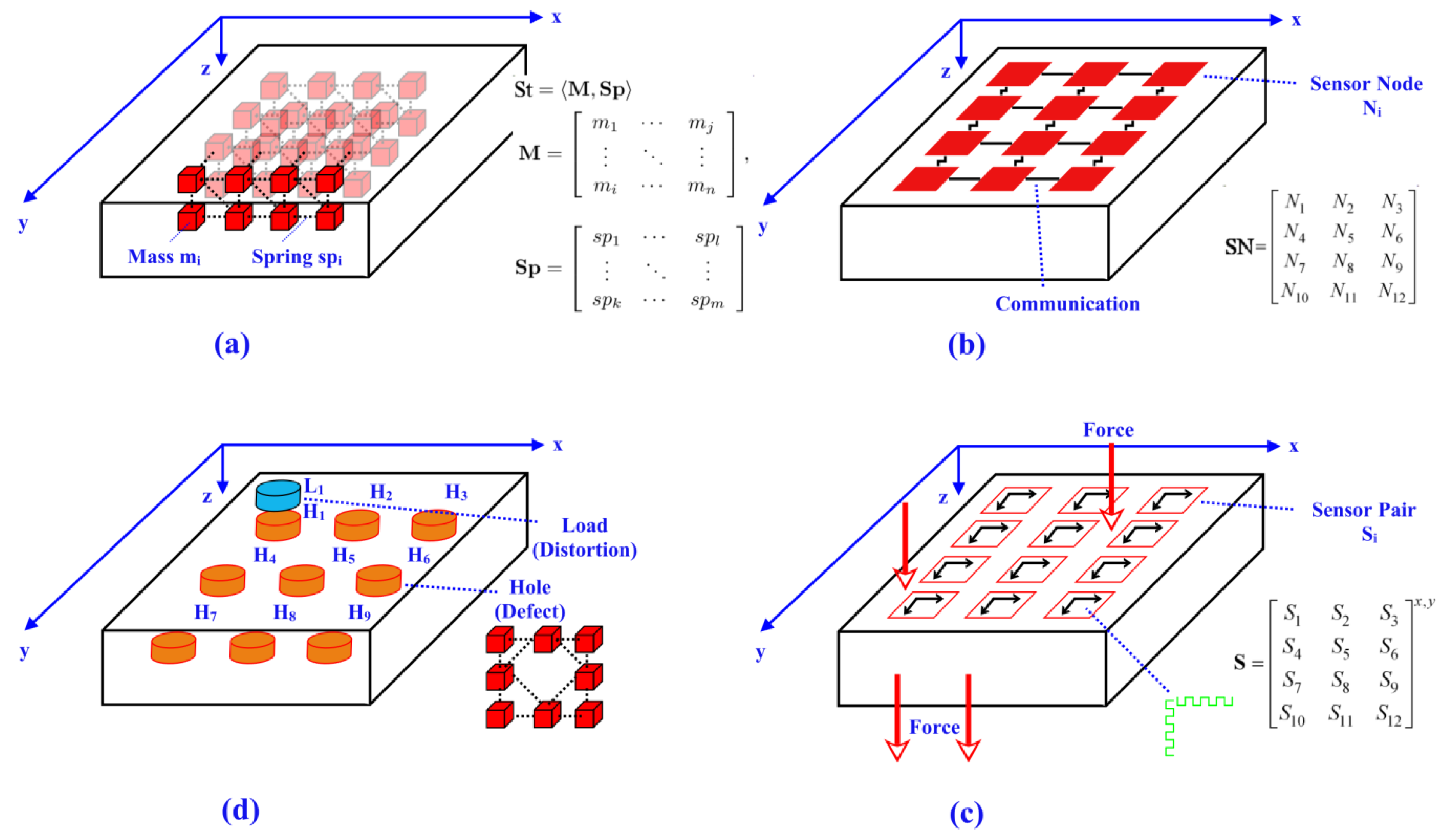
Experiments were performed using the SEJAM2 simulation environment. A rectangular plate was used as a typical device under test (DUT). Two sides of the plate were fixed by two walls. The DUT was modelled with the MBP models and a grid size of 14 × 8 × 3 mass nodes connected with springs (elastic model), shown in Figure 6a. Bending by gravity was used a typical load situation. Starting from an initial state of the DUT, the mass nodes are moved towards the gravity force direction resulting in a typical bending structure.

The sensor network consists of 3 × 4 sensor nodes, shown in Figure 6b. Each node samples two connected synthetic strain-gauge sensors (orthogonal orientated), shown in Figure 6c. The originally undamaged plate DUT can be modified by adding holes inside (by removing mass nodes of the DUT) and prediction can be disturbed by applying additional load to the upper surface, shown in Figure 6d.

The following learning algorithms and models were used:

• Classical decision tree learner (C45);
• Advanced decision tree learner with interval arithmetic and nearest-neighbor approximation (ICE);
• Random forest tree learner (RF);
• Single-layer perceptrons (one layered artificial neural network, SLP);
• Multi-layer perceptrons (deep learning with hidden layers, MLP);
• Multi-label support vector machines (SVM).

Two different learning domain strategies were investigated:

• Global learning with one learner instance (see Figure 4a) using a sensor snapshot (after the DUT dynamics is below a threshold);
• Local learning with 12 node-based learner instances and global fusion (see Figure 4b) using time records of the sensor signals (starting at the beginning of DUT dynamics).

8.1. Global Learning

With 12 sensor nodes and each sensor node connected with a pair of strain gauge sensors, there are 24 input variables. The neural networks consist of 24 input neurons (12 sensor pair feature variables) and 10 output neurons (nine damage locations and the undamaged case). The multi-label SVM consists of 10 parallel binary classifier SVMs (one for each damage feature).

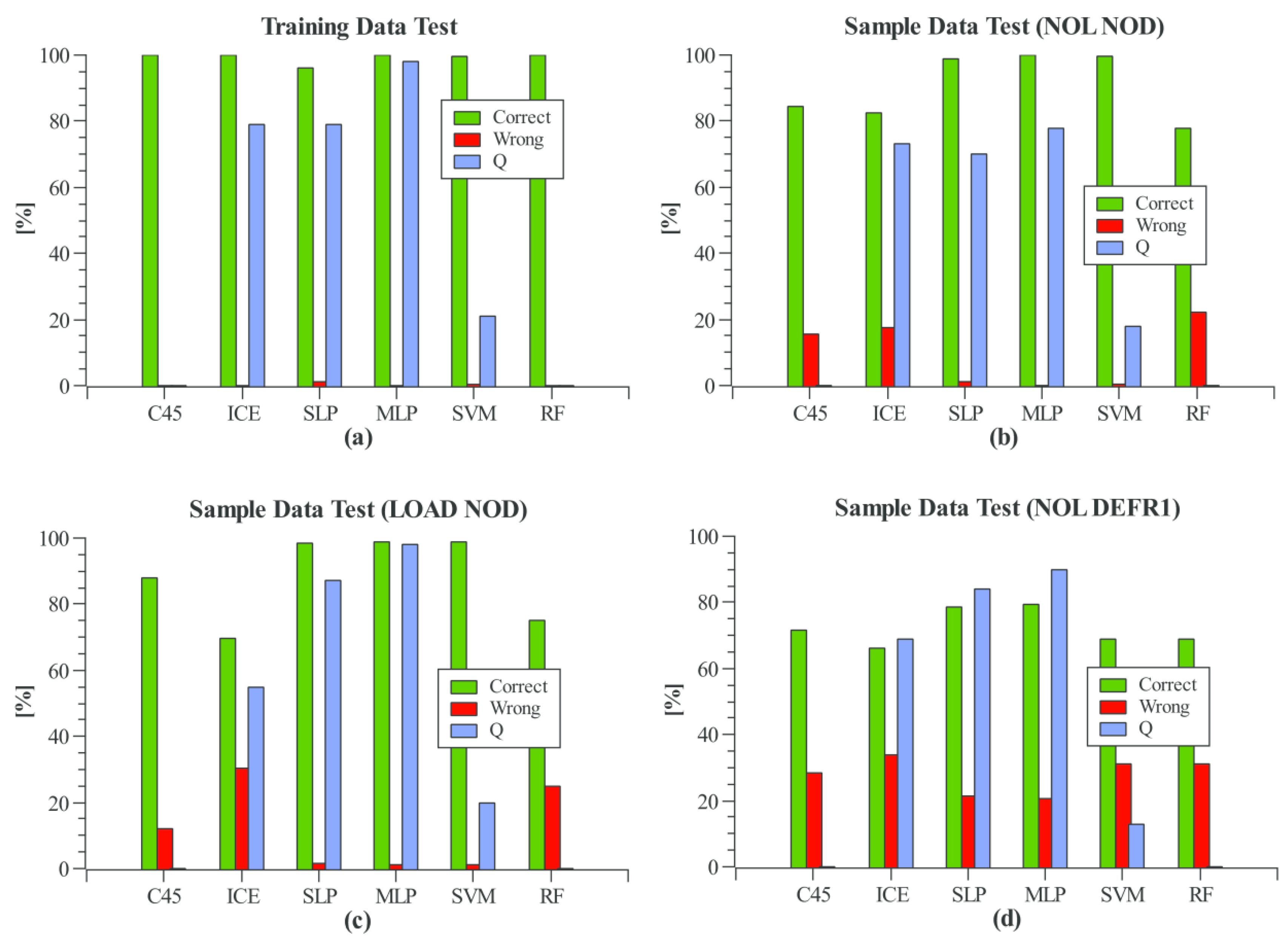
The various ML algorithms differ in learning time and model data size, shown in

Table 3. Comparison of different learned models (200 data sets of all sensors; global learning) showing learning time and model data size.

ML	Parameter	Learning Time	Modelsize (Bytes)
C45	-	8 s	4k
ICE	ε = 0.01	100 ms	16k
SLP	iter = 1000	1 s	190k
MLP1	iter = 1000, layershidden = [5]	2 s	210k
MLP2	iter = 20,000, layershidden = [5]	22 s	210k
SVM	iter = 1000, kernel={type: rbf, C:0.5, σ:0.1}	90 s	260k
RF	depthmax = 10, trees = 5	150 ms	1.2M

for 200 training data sets. The learners require accurate setting of a parameter set (except the C45 learner). The neural networks require the specification of the model architecture (number of hidden layers, number of neurons, and the neuron interconnect graph), whereas the other model architectures are automatically determined by the learner (but still influenced by the learning parameters).

The ICE algorithm has the fastest learning time in the milliseconds scale, followed by the random forest learner. The neural network learners require much higher learning times in order of magnitude of seconds. Adding hidden layers (here only one hidden layer with five neurons) requires a significantly higher amount of learning iterations (about 10–20 times) to get reasonable prediction results. The SLP can be trained with less than 1000 iterations and still results in a high prediction accuracy of about 80%–98% (see Figure 7), whereas a MLP predicts only noise at 1000 iterations. However, the MLP outperforms the SLP if a high training iteration count greater than 10,000 iterations is used, with the disadvantage of high learning times (up to 100 s for 200 training sets). The slowest algorithm in comparison is SVM as result of the binary classifier nature of SVMs. To provide multi-label classification, an SVM is required for the prediction of each label (i.e., here, nine damage locations and the undamaged case label). Although the random forest can compete with the new ICE learner in learning time, the model size is the largest of all compared models and the prediction results are on the lower bound in this comparison.

The computation of the quality confidence marker Q depends in the learned model and algorithm. For neural networks, the output value of the most significant firing output neuron is used (range [0, 1). SVMs usually uses a threshold function to output a binary set of values (e.g., [−1, 1). The output of the SVM before applying the threshold function can be used an approximation of the Q marker, although without no strict and fixed bounds. The classical C45 decision tree and the random forest trees do not deliver any suitable Q marker. In contrast to C45/ID3, the ICE predictor uses nearest neighborhood estimation to find the best matching path in the decision tree. The distance from each node variable value to its nearest child node value is used as Q marker (accumulated over all nodes along a tree search path).

The evaluation results show that the Q confidence marker is not always suitable to give a measure of trust. There is no strong correlation between the Q value and the correctness probability in case of the ICE learner. The MLP results show similar Q values (80%–90%) for training and sample data, but the failure rate in the last situation (defect sensors) is significantly increased. The SVM values for Q are always low (indeed using a best-winner approach selecting the SVM classifier with the highest output but still negative value!).

8.2. Local Learning

In contrast to the previously evaluated global learning approach using sensor snapshots of all spatially distributed sensors at a specific time, the local learning approach uses time-resolved records of the sensor signals with a given capture window (32 samples). Furthermore, each sensor node implements a single-learner instance learning local models that are applied to local sensor data only. Therefore, the input data vector X consists of 64 variables.

There are only two target labels for each learning instance that have to be classified: (DAMAGE) meaning a damage was detected within a region around the sensor node (radius of 1.5 sensor distance lengths) and (NODAMAGE) meaning no damage within this region was detected. In the evaluation, the number of “No damage” cases for each node is much higher than the number of “Damage nearby” cases (naturally).

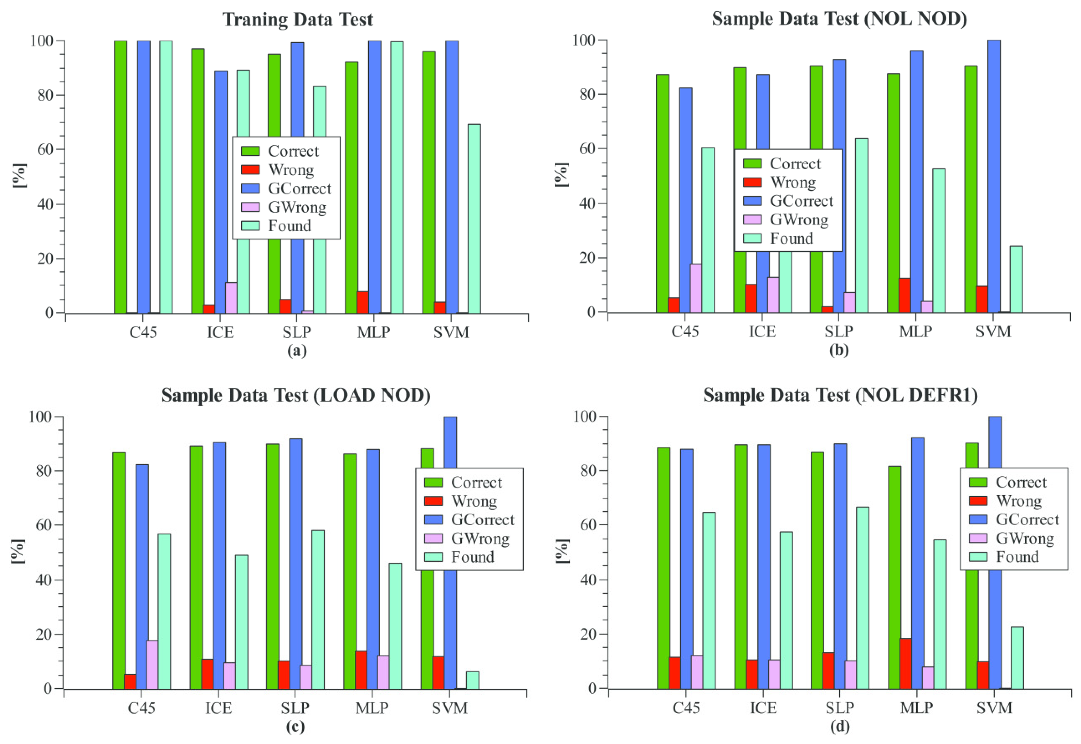
The evaluation of the local learning approach with nine different damage locations and an unmodified structure is shown in Figure 8. Again, training data tests and sample prediction without and with disturbance (additional loads, defect sensors randomly chosen) is shown. Different quality parameters were retrieved from the analysis. The first pair correct/wrong tests each single node whether the damage within the neighboring region was correctly found or not. The second pair gcorrect/gwrong uses global fusion by computing the average position of all sensor nodes detecting a damage. If the average position is near by the real damage location (within a radius of 1.5 node distance units), the classification is counted as correct, otherwise as wrong.

All learning algorithms show a high correct-positive and correct-negative single-node prediction probability with zero or only a few wrong-positive and wrong-negative predictions. However, remember that the NODAMAGE feature has a 10 times higher weight with respect to each single node. The global fused damage prediction quality (with equally distributed weights of the ten different damage features) shows the best result for the SVM learner, although the single local DAMAGE hit rate is rather low compared with the other learners. In contrast to the global learner, the MLP model shows lower prediction quality than the SLP. The decision tree learner can still compete with the more complex neural networks and SVM, leading to a prediction accuracy higher than 80%.

8.3. Efficiency Comparison

The efficiency of a learner is defined by:

$$ϵ=\frac{p}{LD}$$

(7)

where p is the prediction accuracy in %, L is the learning time in seconds, and D is the model data size in kB. In

Table 4. Comparison of efficiencies for different ML algorithms (global learning instance).

C45	ICE	SLP	MLP	SVM	RF
3	50	0.5	0.02	0.004	0.4

, the efficiencies of the different ML algorithms are compared using the results from the previous sections (global learner instance). The prediction accuracy is an average value of all four test cases (training data, sample data, sample data with additional loads, and sample date with random defect sensors).

9. Conclusions

A multi-domain simulation framework realizing tight coupling of physical simulation of mechanical structures and computational simulation of sensor networks was used to investigate different ML approaches and algorithms applied for the prediction of hidden damage. The main focus was to provide a basis for the deployment of low-cost non-calibrated strain gauge sensors towards this aim. It could be shown that simple decision tree models are generally suitable for damage prediction. A new advanced ICE-type decision tree learner was introduced. This learner takes noise of sensor data into consideration leading to improved models and prediction accuracy. Additionally, this new learner outperforms classical decision tree learners and neural networks regarding learning time (in milliseconds) and model data size. A further comparison of single and multi-layer neural networks (deep learning) has revealed no significant advantage over multi-layer networks with respect to prediction accuracy. All learners can be applied in the sensor spatial and time domain, and in centralized single- and multiple-instance decentralized learning architectures. Although SVMs require the highest learning time, they outperform all other algorithms in multiple-instance, decentralized learning architectures using time records of sensor signals. Related to training time and accuracy, the ICE learner provides the best overall efficiency and quality.