TI-Stan: Adaptively Annealed Thermodynamic Integration with HMC ^†

Abstract

We present a novel implementation of the adaptively annealed thermodynamic integration technique using Hamiltonian Monte Carlo (HMC). Thermodynamic integration with importance sampling and adaptive annealing is an especially useful method for estimating model evidence for problems that use physics-based mathematical models. Because it is based on importance sampling, this method requires an efficient way to refresh the ensemble of samples. Existing successful implementations use binary slice sampling on the Hilbert curve to accomplish this task. This implementation works well if the model has few parameters or if it can be broken into separate parts with identical parameter priors that can be refreshed separately. However, for models that are not separable and have many parameters, a different method for refreshing the samples is needed. HMC, in the form of the MC-Stan package, is effective for jointly refreshing the ensemble under a high-dimensional model. MC-Stan uses automatic differentiation to compute the gradients of the likelihood that HMC requires in about the same amount of time as it computes the likelihood function itself, easing the programming burden compared to implementations of HMC that require explicitly specified gradient functions. We present a description of the overall TI-Stan procedure and results for representative example problems.

1. Introduction

Thermodynamic integration (TI) is a numerical technique for evaluating model evidence integrals. The technique was originally developed [2] to estimate the free energy of a fluid. Various improvements and changes have been made over the decades, and the incarnation of the technique that our method is based on is the adaptively-annealed, importance sampling-based method described by Goggans and Chi [3]. Their implementation follows John Skilling’s BayeSys [4], and both make use of Binary slice sampling (BSS) and the Hilbert curve to complete the implementation. This article proposes a modification of this method that uses PyStan [5,6] and the No U Turn Sampler (NUTS) [7] instead of BSS and the Hilbert curve. This article is an adaptation of portions of the first author’s doctoral dissertation ([1] Chapter 3). A Python 3 implementation of this method by the authors can be found on GitHub (https://github.com/rwhender/ti-stan) [8].

1.1. Motivation

The family of adaptively-annealed TI methods are important for solving model comparison problems in engineering, where we frequently need to evaluate complex physics-based mathematical models. TI methods with fixed annealing schedules (e.g., [9,10]) are useful for solving more traditional statistics problems, but tend to fail with the complex models that arise in engineering problems. TI methods that use BSS on the Hilbert curve are useful for a large set of problems; however, these methods see diminishing returns when the number of model parameters grows somewhat large ($>10$ or so). These performance issues can be mitigated if the model equation can be decomposed into additive components with identical form and equivalent joint priors on their parameters. However, for problems with many model parameters and with model equations that cannot be decomposed, a different class of methods is required.

1.2. Background

From Bayes’ theorem, for model vector $\mathit{M}$, data vector $\mathit{D}$, model parameter vector $\mathsf{\Theta }$, and prior information I, the model evidence is

$$\mathrm{p}\left(\mathit{D}\right|\mathit{M},I)=\int \mathrm{p}(\mathit{D}|\mathsf{\Theta },\mathit{M},I)\mathrm{p}\left(\mathsf{\Theta }\right|\mathit{M},I)\mathrm{d}\mathsf{\Theta }.$$

(1)

Here we introduce an inverse temperature parameter, $\beta$, that will control how much the likelihood influences the evidence value,

$$\mathrm{p}\left(\mathit{D}\right|\mathit{M},\beta ,I)=\int {\left[\mathrm{p}\left(\mathit{D}\right|\mathsf{\Theta },\mathit{M},I)\right]}^{\beta }\mathrm{p}\left(\mathsf{\Theta }\right|\mathit{M},I)\mathrm{d}\mathsf{\Theta }.$$

(2)

The full derivation is omitted here. The result is the thermodynamic integral form of the model evidence,

$$log\mathrm{p}\left(\mathit{D}\right|\mathit{M},\beta ,I)=-{\int }_0^1{〈E_L\left(\mathsf{\Theta }\right)〉}_{\beta }\mathrm{d}\beta ,$$

(3)

where the energy term is defined as the negative log-likelihood:

$$E_L\left(\mathsf{\Theta }\right)=-log\mathrm{p}\left(\mathit{D}\right|\mathsf{\Theta },\mathit{M},I).$$

(4)

The integral in (3) usually cannot be evaluated analytically. For problems with relatively simple models, a fixed temperature ladder can be used, and Markov chain Monte Carlo (MCMC) can be used to estimate the expected energy at each temperature. However, for the class of problems we are concerned with, an approach in which the subsequent temperature is computed based on the conditions observed in the current step is necessary. This process is known as adaptive annealing. The general procedure as described by [3] is as follows:

1.

Start at $\beta =0$ where $\mathrm{p}\left(\mathsf{\Theta }\right|\mathit{M},\mathit{D},\beta ,I)=\mathrm{p}(\mathsf{\Theta }|\mathit{M},I)$, and draw C samples from this distribution (the prior).

2.

Compute the Monte Carlo estimator for the expected energy at the current $\beta$,

$${〈E_L\left(\mathsf{\Theta }\right)〉}_{\beta }\approx \frac{1}{N}\sum _{t=1}^C{E}_L\left({\mathsf{\Theta }}_t\right),$$

(5)

where ${\mathsf{\Theta }}_t$ is the current position of the t-th Markov chain.

3.

Increment $\beta$ by $\mathsf{\Delta }{\beta }_i$, where

$$\mathsf{\Delta }{\beta }_i=\frac{log\frac{max w_j}{min w_j}}{max{E}_L\left({\mathsf{\Theta }}_{\mathit{i}}\right)-min{E}_L\left({\mathsf{\Theta }}_{\mathit{i}}\right)},$$

(6)

j is the index on the chains, $w_j$ is the weight associated with chain j, and

$$w_j=exp[-\mathsf{\Delta }{\beta }_i{E}_L\left({\mathsf{\Theta }}_{\mathbf{j}}\right)].$$

(7)

4.

Re-sample the population of samples using importance sampling.

5.

Use MCMC to refresh the current population of samples. This yields a more accurate sampling of the distribution at the current temperature. This step can be easily parallelized, as each sample’s position can be shifted independently of the others.

6.

Return to step 2 and continue until ${\beta }_i$ reaches 1.

7.

Estimate (3) using quadrature and the expected energy estimates built up using (5).

In this procedure, steps 3 and 4 are closely connected. In order to refresh the sample population most effectively, the importance sampling step should discard and replace at most 1 sample per temperature. New temperatures are chosen in a way that encourages this behavior. The term $log\frac{max w_j}{min w_j}$ is a method parameter that can be set to make the adaptive annealing process more or less aggressive. Values of this parameter only slightly greater than one encourage a slow annealing, while higher values encourage a faster process.

2. Materials and Methods

The main innovation of this article relates to the implementation of step 5. As of Summer 2018, a survey of the available modern implementations of MCMC methods indicated that MC Stan (or simply Stan) [5], was the gold standard for general purpose MCMC. Stan uses NUTS [7] as the basis for its sampling functions. NUTS is based on Hamiltonian Monte Carlo (HMC) [11], which uses the gradient of the log-likelihood function to more efficiently explore the posterior distribution. NUTS improves upon HMC by automatically choosing optimal values for HMC’s tunable method parameters. NUTS has been shown to sample complex distributions effectively. We sought to build an improved thermodynamic integration implementation by using Stan instead of binary slice sampling and leapfrog sampling to refresh the sample population at each temperature within TI. The result, Thermodynamic integration with Stan (TI-Stan), is described in this section.

The TI-Stan algorithm is shown in Algorithm 1.

Our implementation is in Python, so we made use of the PyStan interface to Stan [6]. Stan defines its own language for defining statistical models, which allows it to efficiently compute the derivatives needed for HMC via automatic differentiation. For a particular problem, it is therefore necessary to write a Stan file that contains the Stan-formatted specification of the model, in addition to the pure-Python energy functions necessary for TI with BSS. Once one is familiar with the simple Stan language, this additional programming cost becomes trivial compared to the time savings achieved by using this method instead of BSS.

Algorithm 1 Thermodynamic integration with Stan

1: procedureTI($P,S,C,W,data$) 2:     Inputs: P–Number of parameters, S–Number of Stan iterations per temperature, C–Number of chains, W–Ratio to control adaptive annealing, $data$–Data 3:     for $m\leftarrow 1,C$ do 4:      for $j\leftarrow 1,P$ do 5:      ${\alpha }_j^m\leftarrow {\mathrm{R}}_{\mathrm{AND}}(0,1)$ 6:      end for 7:      $E_m^{*}\leftarrow {\mathrm{E}}_{\mathrm{NERGY}}({\alpha }^m,data)$ 8:     end for 9:     $i\leftarrow 1$ 10:    Compute ${\langle E^{*}\rangle }_i$ 11:    ${\beta }_1\leftarrow min\{log\left(W\right)/[max\left(E^{*}\right)-min\left(E^{*}\right)],1\}$ 12:    $w\leftarrow exp(-{\beta }_1{E}^{*})$ 13:    ${\mathrm{I}}_{\mathrm{MPORTANCE}}{\mathrm{S}}_{\mathrm{AMPLING}}(w,\alpha ,E^{*},C)$ 14:    while ${\beta }_i>0$ and ${\beta }_i<1$ do 15:      for $m\leftarrow 1,C$ do 16:      ${\mathrm{S}}_{\mathrm{TAN}}{\mathrm{S}}_{\mathrm{AMPLING}}({\alpha }^m,E_m^{*},C,P,S,{\beta }_i,data)$ 17:      end for 18:      $i\leftarrow i+1$ 19:      $\mathsf{\Delta }\beta \leftarrow log\left(W\right)/[max\left(E^{*}\right)-min\left(E^{*}\right)]$ 20:      ${\beta }_i\leftarrow min({\beta }_{i-1}+\mathsf{\Delta }\beta ,1)$ 21:      if ${\beta }_{i-1}+\mathsf{\Delta }\beta >1$ then 22:      $\mathsf{\Delta }\beta \leftarrow 1-{\beta }_{i-1}$ 23:      end if 24:      $w\leftarrow exp(-\mathsf{\Delta }\beta E^{*})$ 25:      ${\mathrm{I}}_{\mathrm{MPORTANCE}}{\mathrm{S}}_{\mathrm{AMPLING}}(w,\alpha ,E^{*},C)$ 26:    end while 27:    Estimate (3) using trapezoid rule and $\left\{{\beta }_i\right\}$ and $\left\{{\langle E^{*}\rangle }_i\right\}$ 28: end procedure

2.1. Tests

We use two test problems to demonstrate TI-Stan in practice. These test problems are described below.

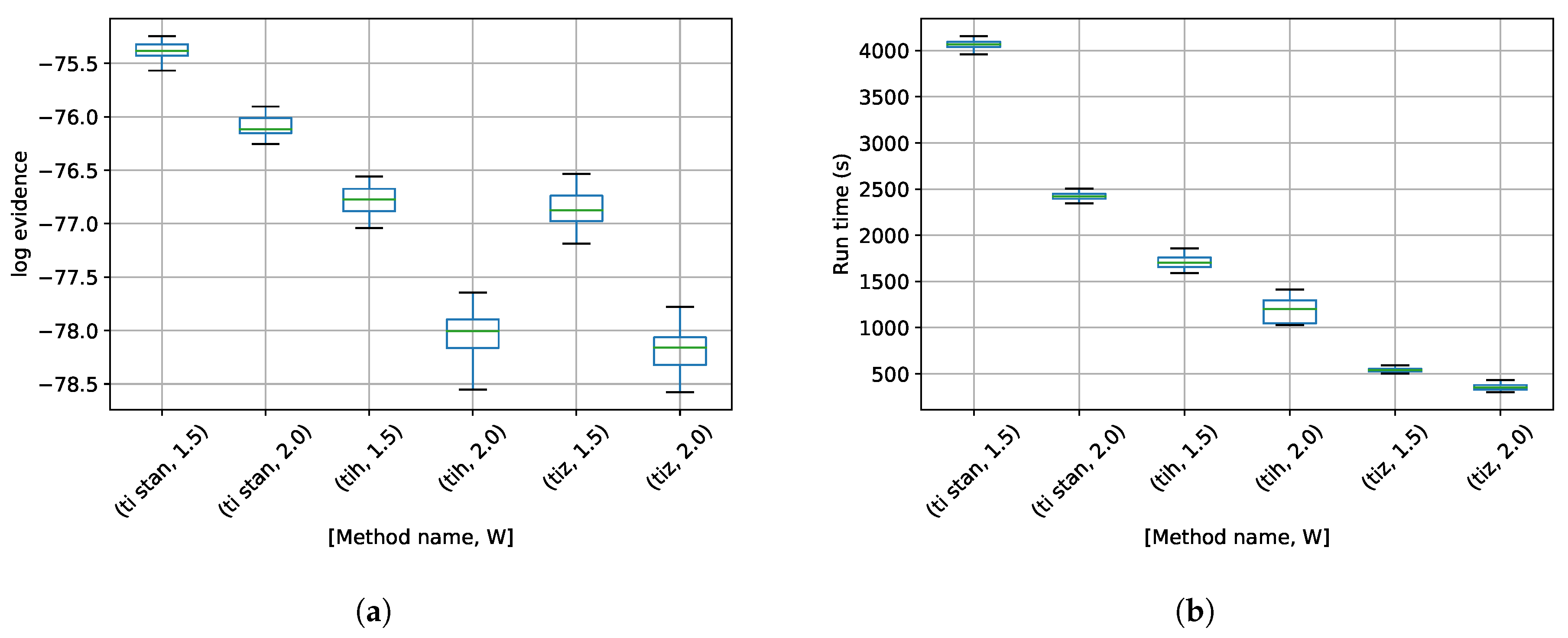
2.1.1. Twin Gaussian Shells

The first example is the twin Gaussian shell problem from [12]. In [12], the authors present results for this problem in up to 30 dimensions. Handley, et al. [13] also use this problem in 100 dimensions to test their algorithm. This problem presents a few interesting challenges. Because the likelihood takes the form of a thin, curved density whose mass centers on a hyper-spherical shell, MCMC moves are difficult to make efficiently. The bimodal distribution is also challenging to sample effectively. Finally, the examples we explore are high-dimensional to the point that standard numerical integration techniques would be useless.

The likelihood function in the twin Gaussian shells problem takes the form,

$$\mathcal{L}\left(\mathsf{\Theta }\right)=\frac{1}{\sqrt{2\pi }{w}_1}exp\left[-\frac{\left(\right|\mathsf{\Theta }-{\mathbf{c}}_1{|-r_1)}^2}{2w_1^2}\right]+\frac{1}{\sqrt{2\pi }{w}_2}exp\left[-\frac{\left(\right|\mathsf{\Theta }-{\mathbf{c}}_2{|-r_2)}^2}{2w_2^2}\right].$$

(8)

Following [12], we set the parameters as follows: $w_1=w_2=0.1$, $r_1=r_2=2$, ${\mathbf{c}}_1={[-3.5,0,\cdots ,0]}^T$, and ${\mathbf{c}}_2={[3.5,0,\cdots ,0]}^T$. We use a uniform prior over the hypercube that spans $[-6,6]$ in each dimension.

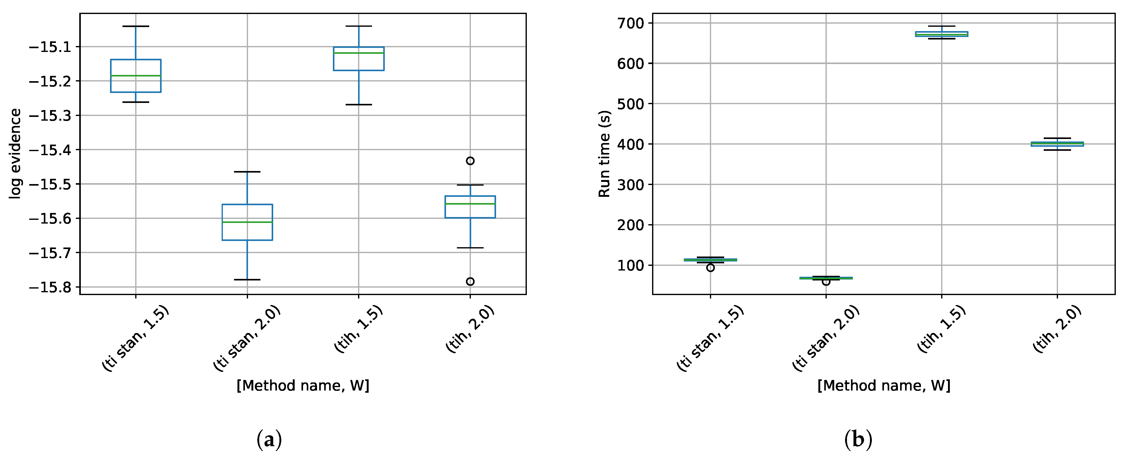
2.1.2. Detection of Multiple Stationary Frequencies

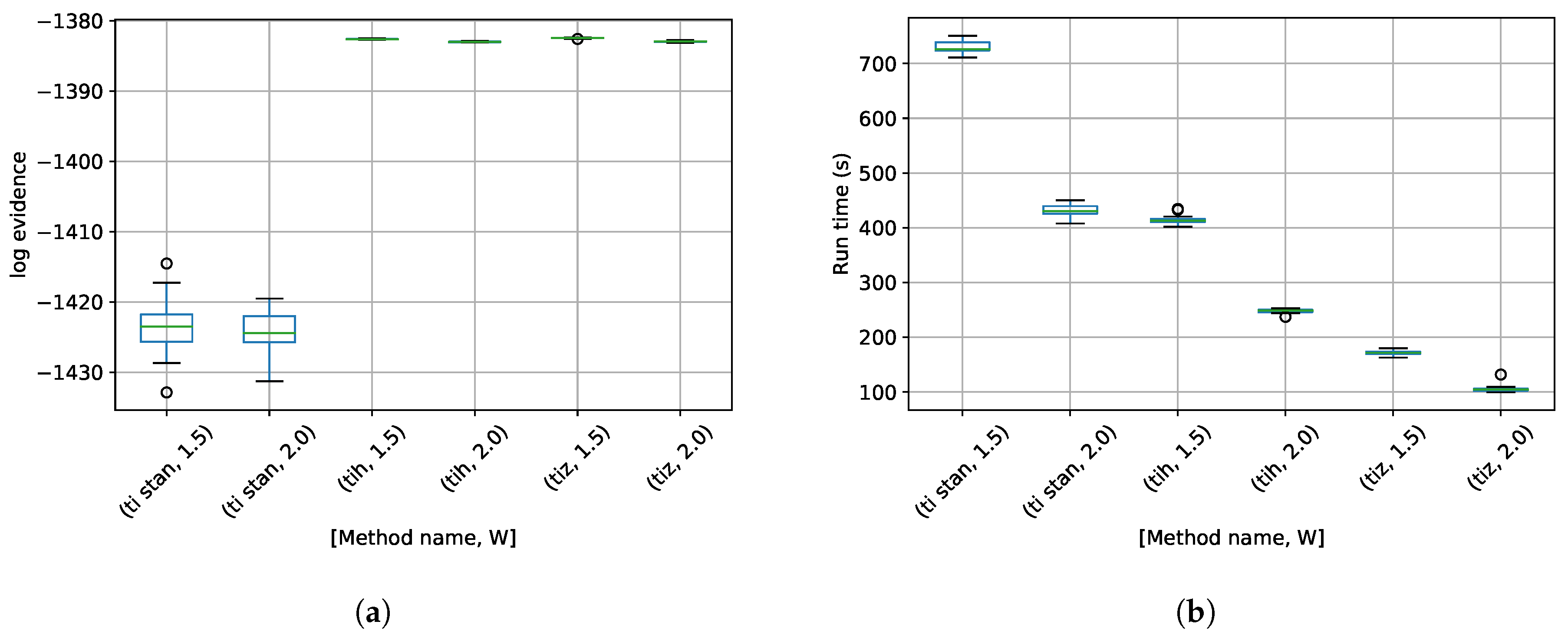
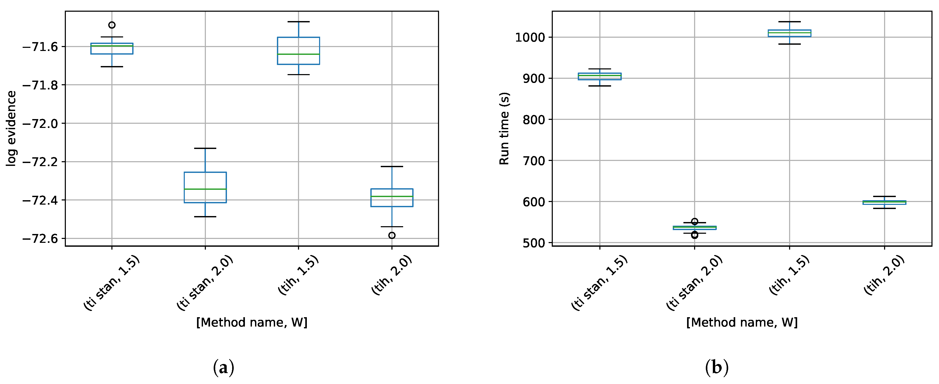
For the second test, we estimate the number of stationary frequencies present in a signal. This problem is similar to the problem of multiple stationary frequency estimation in [14, Chapter 6], with the additional task of determining the number of stationary frequencies present. Differences among log-evidence values for models containing either the most probable number of frequencies or more tend to be small, meaning that a precise estimate of these log-evidence values is essential to the task of determining the most probable model.

Each stationary frequency (j) in the model is determined by three parameters: the in-phase amplitude ($A_j$), the quadrature amplitude ($B_j$), and the frequency ($f_j$). Given J stationary frequencies, the model at time step $t_i$ takes the following form:

$$g\left[t_i;\mathsf{\Theta }\right]=\sum _{j=1}^J{A}_{j}cos\left(2\pi f_j{t}_i\right)+B_{j}sin\left(2\pi f_j{t}_i\right),$$

(9)

where $\mathsf{\Theta }$ is the parameter vector

$$\mathsf{\Theta }={\left[A_1{B}_1{f}_1\cdots A_J{B}_J{f}_J\right]}^T.$$

For the purposes of this test the noise variance used to generate the simulated data is known, hence we use a Gaussian likelihood function,

$$\mathcal{L}\left(\mathsf{\Theta }\right)=\prod _{i=1}^{K}exp\left\{-\frac{{\left[g\left(t_i;\mathsf{\Theta }\right)-d_i\right]}^2}{2{\sigma }^2}\right\},$$

(10)

for K simulated data $d_i$ and noise variance ${\sigma }^2$. The log-likelihood function is then

$$log\mathcal{L}\left(\mathsf{\Theta }\right)=-\sum _{i=1}^K\frac{{\left[g\left(t_i;\mathsf{\Theta }\right)-d_i\right]}^2}{2{\sigma }^2}.$$

(11)

Each model parameter is assigned a uniform prior distribution with limits as shown in

Table 1. Prior bounds for multiple stationary frequency model parameters.

	Lower Bound	Upper Bound
$A_j$	$-2$	2
$B_j$	$-2$	2
$f_j$	0 Hz	$6.4$ Hz

.

Our test signal is a sum of two sinusoidal components, and zero-mean Gaussian noise with variance ${\sigma }^2=0.01$. This signal is sampled at randomly-spaced instants of time, in order to demonstrate that this time-domain method does not require uniform sampling to perform spectrum estimation. Bretthorst [15] demonstrates that the Nyquist critical frequency in the case of nonuniform sampling is $1/2\mathsf{\Delta }{T}^{\prime }$, where $\mathsf{\Delta }{T}^{\prime }$ is the dwell time. The dwell time is not defined for arbitrary-precision time values as used in this example, so we must choose another limiting value. A more conservative limit is given by $1/10\mathsf{\Delta }{T}_{\mathrm{avg}}$, where $\mathsf{\Delta }{T}_{\mathrm{avg}}$ is the average spacing between time steps, $1/64$ s. This formulation yields a prior maximum limit of $6.4$ Hz, as shown in Table 1. The parameters used to generate the simulated data are shown in

Table 2. Parameters used to generate simulated signal.

j	${\mathit{A}}_{\mathit{j}}$	${\mathit{B}}_{\mathit{j}}$	${\mathit{f}}_{\mathit{j}}$ (Hz)
1	$1.0$	$0.0$	$3.1$
2	$1.0$	$0.0$	$5.9$

.

3. Results

For these tests, performance is compared among the Thermodynamic integration with binary slice sampling (TI-BSS) method and the TI-Stan method. The settings used for TI-BSS are shown in

Table 3. Parameters for TI-BSS examples.

Parameter	Value	Definition
S	200	Number of binary slice sampling steps
M	2	Number of combined binary slice sampling and leapfrog steps
C	256	Number of chains
B	32	Number of bits per parameter in SFC

, while the settings used for TI-Stan are shown in

Table 4. Parameters for TI-Stan examples.

Parameter	Value	Definition
S	200	Number of steps allowed in Stan
C	256	Number of chains

. For each example, the user-defined annealing control constant W was set to both 1.5 and 2.0. For the box-plots in this section, the middle line represents the median value, the box is bounded by the upper and lower quartiles, and the whiskers extend to the range of the data that lies within 1.5 times the inter-quartile range. Any data points past this threshold are plotted as circles.

These results were generated on a Google Cloud instance with 32 virtual Intel Broadwell CPUs and 28.8 GB of RAM.

First, we present results for the twin Gaussian shells distribution with 10 dimensions. A box-plot summarizing the log-evidence estimates over 20 runs each for TI-Stan and Thermodynamic integration with binary slice sampling and the Hilbert curve (TI-BSS-H) and for each value of W is shown in Figure 1a. A box-plot summarizing the run times over 20 runs each for the TI methods is shown in Figure 1b.

Second, we present results for the detection of multiple stationary frequencies problem. Box-plots of log-evidence values for a model assuming one, two, and three frequencies present are shown in Figure 2a, Figure 3a, and Figure 4a. For the models with one and three frequencies present, results are shown for TI-Stan, TI-BSS-H, and Thermodynamic integration with binary slice sampling and the Z-order curve (TI-BSS-Z) [16]. For the model with two frequencies present (the model also used to generate the test signal), results for TI-BSS-Z are not shown. For this model, TI-BSS-Z ended early here and did not arrive at a reasonable result. Box-plots of the run time for models assuming one, two, and three frequencies present are shown in Figure 2b, Figure 3b, and Figure 4b.

4. Discussion

Regarding the twin Gaussian shells test, the analytical log-evidence for this distribution [12] is $-14.59$. None of the configurations tested actually reached that value (Figure 1a, but the runs using $W=1.5$ got closest, suggesting that a value of W closer to 1 would perhaps approach the correct value more closely. Figure 1b shows that the run time drastically increases as W approaches 1. It also shows that TI-BSS-H takes about 6 times longer, on average, than TI-Stan to compute its estimate of the log-evidence. According to Figure 1a, the two methods have comparable accuracy and precision, so this difference in run time illustrates the difficulty the Hilbert curve-based method has with distributions of high dimension.

Regarding the detection of multiple stationary frequencies test, there are no analytical log-evidence values available. We argue that a method is successful if the model used to generate the data clearly has the highest log-evidence, with a good margin between it and the log-evidence for the other models. Figure 2a and Figure 4a show some significant disagreement among the various methods for the “wrong” models (those with one and three frequencies), but Figure 3a shows that the methods are in much closer agreement for the two frequency model. For TI-Stan and TI-BSS-H and for both values of W, the two frequency model is clearly the maximum-log-evidence choice. Even with the variations in the runs, the results do not overlap at any point from model to model, and the closest model-to-model margins are all greater than 2.3, which corresponds to an odds of 10.

In Figure 2b, TI-Stan has the greatest run time for both values of W, suggesting that its adaptive sampling process had trouble efficiently sampling distributions based on this high-error model. TI-BSS-H was much faster, and TI-BSS-Z was faster still. In Figure 3b, the run times of TI-Stan and TI-BSS-H are comparable. This suggests that TI-Stan was able to more effectively sample the distribution based on the lower-error model. Figure 4b shows a similar pattern in the run times to Figure 2b. The fact that this model is able to fit the noise in the data (yielding especially sharp distributions) and the fact that the distribution is increasingly multi-modal as the number of frequencies increases may explain why TI-Stan took a long time to compute a result here.

These preliminary results indicate that TI-Stan is a promising method for computing model evidence for problems with complex physics-based mathematical models. Results for further problems, including the twin Gaussian shell problem with up to 100 dimensions, can be found in ([1] Chapter 3). Future work could further evaluate this method’s usefulness by solving real complex model comparison problems in engineering.

References

1. Henderson, R.W. Design and analysis of efficient parallel bayesian model comparison algorithms. Doctoral Dissertation, University of Mississippi, Oxford, MS, USA, 2019. [Google Scholar]
2. Kirkwood, J.G. Statistical Mechanics of Fluid Mixtures. J. Chem. Phys. 1935, 3, 300–313. [Google Scholar] [CrossRef]
3. Goggans, P.M.; Chi, Y. Using thermodynamic integration to calculate the posterior probability in Bayesian model selection problems. AIP Conf. Proc. 2004, 707, 59–66. [Google Scholar] [CrossRef]
4. Skilling, J. BayeSys and MassInf; Maximum Entropy Data Consultants Ltd.: London, UK, 2004. [Google Scholar]
5. Carpenter, B.; Gelman, A.; Hoffman, M.D.; Lee, D.; Goodrich, B.; Betancourt, M.; Brubaker, M.; Guo, J.; Li, P.; Riddell, A. Stan : A Probabilistic Programming Language. J. Stat. Softw. 2017, 76. [Google Scholar] [CrossRef] [PubMed]
6. Stan Development Team. PyStan: The Python Interface to Stan. 2018. Available online: http://mc-stan.org (accessed on 21 November 2019).
7. Hoffman, M.D.; Gelman, A. The No-U-Turn Sampler: Adaptively Setting Path Lengths in Hamiltonian Monte Carlo. J. Mach. Learn. Res. 2014, 15, 1593–1623. [Google Scholar]
8. Henderson, R.W. TI-Stan. 2019. original-date: 2019-07-04T09:56:19Z. Available online: https://github.com/rwhender/ti-stan. (accessed on 21 November 2019).
9. Gelman, A.; Meng, X.L. Simulating normalizing constants: From importance sampling to bridge sampling to path sampling. Stat. Sci. 1998, 13, 163–185. [Google Scholar] [CrossRef]
10. Oates, C.J.; Papamarkou, T.; Girolami, M. The Controlled Thermodynamic Integral for Bayesian Model Evidence Evaluation. J. Am. Stat. Assoc. 2016, 111, 634–645. [Google Scholar] [CrossRef]
11. Neal, R.M. MCMC using Hamiltonian dynamics. In Handbook of Markov Chain Monte Carlo; Brooks, S., Gelman, A., Jones, G., Meng, X.L., Eds.; Chapman & Hall / CRC Press: New York, NY, USA, 2011. [Google Scholar]
12. Feroz, F.; Hobson, M.P.; Bridges, M. MultiNest: an efficient and robust Bayesian inference tool for cosmology and particle physics. Mon. Not. R. Astron. Soc. 2009, 398, 1601–1614. [Google Scholar] [CrossRef]
13. Handley, W.; Hobson, M.; Lasenby, A. PolyChord: Next-generation nested sampling. Mon. Not. R. Astron. Soc. 2015, 453, 4384–4398. [Google Scholar] [CrossRef]
14. Bretthorst, G.L. Bayesian Spectrum Analysis and Parameter Estimation; Springer: Berlin/Heidelberg, Germany, 1988. [Google Scholar]
15. Bretthorst, G.L. Nonuniform sampling: Bandwidth and aliasing. AIP Conf. Proc. 2001, 567, 1–28. [Google Scholar] [CrossRef]
16. Henderson, R.W.; Goggans, P.M. Using the Z-order curve for Bayesian model comparison. In Bayesian Inference and Maximum Entropy Methods in Science and Engineering. MaxEnt 2017; Springer Proceedings in Mathematics & Statistics; Polpo, A., Stern, J., Louzada, F., Izbicki, R., Takada, H., Eds.; Springer: Berlin/Heidelberg, Germany, 2018; Volume 239, pp. 295–304. [Google Scholar]
Figure 1. Twin Gaussian shell test results. (a) Box-plot of log-evidence for the 10-D twin Gaussian shell problem for TI-Stan and TI-BSS-H; (b) Box-plot of run time in seconds for the 10-D twin Gaussian shell problem for TI-Stan and TI-BSS-H.
Proceedings 33 00009 g001
Figure 2. MSF model with J = 1 results. (a) Box-plot of log-evidence for the one stationary frequency model for TI-Stan, TI-BSS-H, and TI-BSS-Z, for two values of W; (b) Box-plot of run time for the one stationary frequency model for TI-Stan, TI-BSS-H, and TI-BSS-Z, for two values of W.
Proceedings 33 00009 g002
Figure 3. MSF model with J = 2 results. (a) Box-plot of log-evidence for the two stationary frequency model for TI-Stan and TI-BSS-H, for two values of W; (b) Box-plot of run time for the two stationary frequency model for TI-Stan and TI-BSS-H, for two values of W.
Proceedings 33 00009 g003
Figure 4. MSF model with J = 1 results. (a) Box-plot of log-evidence for the three stationary frequency model for TI-Stan, TI-BSS-H, and TI-BSS-Z, for two values of W; (b) Box-plot of run time for the three stationary frequency model for TI-Stan, TI-BSS-H, and TI-BSS-Z, for two values of W.
Proceedings 33 00009 g004