Abstract
Hyperspectral datasets provide explicit ground covers with hundreds of bands. Filtering contiguous hyperspectral datasets potentially discriminates surface features. Therefore, in this study, a number of spectral bands are minimized without losing original information through a process known as dimensionality reduction (DR). Redundant bands portray the fact that neighboring bands are highly correlated, sharing similar information. The benefits of utilizing dimensionality reduction include the ability to slacken the complexity of data during processing and transform original data to remove the correlation among bands. In this paper, two DR methods, principal component analysis (PCA) and minimum noise fraction (MNF), are applied to the Airborne Visible/Infrared Imaging Spectrometer-Next Generation (AVIRIS-NG) dataset of Kalaburagi for discussion.
1. Introduction
Hyperspectral sensor images are employed in various applications of remote sensing, containing spatial and spectral information about the surface of the Earth. These images are acquired from both airborne and spaceborne platforms, rendering data with high spectral resolution, narrow contiguous bands that are redundant and complex to process [1]. In order to reduce the complexity of the data, various transforms have been applied to scale and adjust the image data, thus eliminating the noise from each band [2]. Transforms like principal component analysis (PCA), minimum noise fraction (MNF), and independent component analysis (ICA), produce new components that are ordered by image quality. Such dimensionality reduction (DR) techniques are applied to raw datasets for effective noise removal and intense smoothening is employed for components with a high noise and low signal content foreach band of the original data [3]. Furthermore, techniques like optimized MNF (OMNF), which calculates the noise covariance matrix (NCM) via spatial spectral de-correlation (SSDC), perform spectral unmixing, producing components for better classification. The inherent dimensionalities of bands are resolved for a visual inspection of the eigenvalues that are further utilized for the endmember extraction process [4]. Determining an appropriate and evident DR technique is still a tough task while handling hyperspectral imageries. Despite some disadvantages, PCA is a commonly used DR technique as it has a significant effect on classification. Classification results are greatly influenced by MNF when the ground cover features exhibit homogeneity. The efficiency of the classifiers improves with reduced components that reveal apparently informative bands [5,6]. This paper compares and evaluates the performance of two defined DR methods, namely PCA and MNF, by interpreting the eigen values acquired during processing. The cumulative variances of reduced components are explored for bands showing high correlation to low-order bands containing noise affecting the quality of the original hyperspectral imagery. Bands comprising definite and high information an be further utilized for processing.
2. Material and Methods
2.1. Dataset Used
The Airborne Visible/Infrared Imaging Spectrometer-Next Generation (AVIRIS-NG) hyperspectral dataset for a portion of the Kalaburagi region, Karnataka, with a total extent from 76°04’ to 77°42’ East longitude, and 17°12’ to17°46’ North latitude, was used in this study. AVIRIS-NG provides a spectrum of 432 bands ranging from a wavelength of 376–2500 nm. The dataset is atmospherically corrected to obtain the reflectance spectrum of 425 bands, which can then be employed for detailed processing.
2.2. Methodology
The dimensionality reduction method applied for the dataset is explained in the following subsections.
2.2.1. Optimal Band Selection through Dimensionality Reduction
Determination of the DR method is a challenging job for simplifying the process. For the selected hyperspectral AVIRIS-NG dataset shown in Figure 1, PCA and MNF were applied to find the intrinsic dimensions that clearly disclose urban areas of the considered study region. From the correlation matrix computed and the derived eigenvalues, a scree plot was graphically procured for additional information. Through a visual observation of the eigen images, the components that provide useful details with less noise that are ordered from high to low were taken into account. Appropriate band selection through PCA and MNF is briefly described.
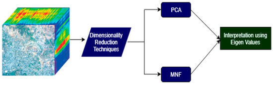
Figure 1.
Workflow.
2.2.2. Principal Component Analysis
PCA is a preprocessing linear transformation technique that reorganizes the variance from multiple bands to a new set of bands. Input bands processed after PCA provide uncorrelated bands that have maximized data variance. In this study, for the given hyperspectral data, statistics representing the covariance and correlation matrix were computed. The process of PC rotation normalizes the calculated matrices to unit variance and in order to equalize the influence of bands, it reduces the bands with higher variance and vice versa [7].In general, the PC finds the relationship between dependent and independent variables that prioritizes them, in which the first principal component spreads along a straight line with the longest dimension of the data and the second component is projected perpendicular to it, thus fitting the error produced by the first component. After fitting the principal components to the variance of the data, eigenvalues and eigenvectors can be assessed [8]. The goal of this study is to reduce the n dimensional data that is projected into a k dimensional subspace in which k < n is implemented, through which informative bands are retained, thus increasing the computational accuracy. Bands ranging from λ50 = 621.87 nm to λ194 = 1343.11 nm, λ224 = 1493.37 nm to λ280 = 1773.86 nm, and λ335 = 2049.34 nm to λ395 = 2349.86 nm, resulting in a total of 263 spectral bands where λk is the kth spectral band with its corresponding wavelength, were chosen by avoiding unessential bands. With respect to the eigenvalues, the first nine components that render information from the dataset were considered for analysis.
2.2.3. Minimum Noise Fraction
Noise characteristics change from band to band and provide coarsely ordered bands as per the image quality. The MNF transform discussed in this paper has the capability of providing optimal high to low order to the bands with respect to the image quality. MNF defines how the spatial information can be used to interpret the covariance structure of the signal and noise. The transform segregates the image in the data and its inherent dimensionality through two cascaded PC transformations. At first, the noise covariance matrix is computed to decorrelate and rescale the noise from the data, known as ‘noise whitening’. A later process is eigen decomposition on the modified matrix, which orders the bands with respect to the signal to noise. Higher eigenvalues (>1) contain more information in the bands and values near 1 render noisy datasets. Similar to the PCA, the top components are filtered for the study and the rest are zeroed out [9]. A total number of 263 spectral bands considered for PCA were taken into account for applying the MNF transform.
3. Results and Discussion
3.1. Transformation Results
DR techniques retrieve information that can be further processed for endmember extraction and classification. From the results, it is evident that noise from the data is segregated, although bands are ordered by a decreasing signal to noise ratio. It is observed that the first nine components of each transform render highly informative bands from the eigenvalues displayed. Bands that comprise urban information are clearly seen in PCA-transformed bands of 1, 3, 5, and 9 and MNF-transformed bands of 1, 4, 7, and 8. The rest of the components also comprise details, along with greatly enhanced noise patterns. It is noted that there is a much lower noise concentration and less correlation between the bands with shorter wavelengths. The remaining bands have a salt and pepper noise effect, thus slackening the quality of the transformed image. Clean transformed band information was retrieved through linear transformation with respect to the reflectance characteristics of each band, providing noise-free components for further data analysis processing. Figure 2 and Figure 3 show the dimensionally-reduced bands resulting from the application of PCA and MNF, respectively.
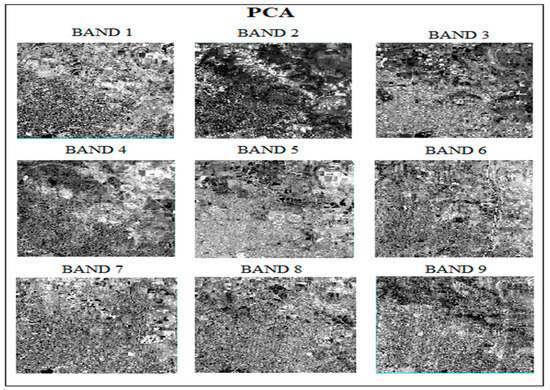
Figure 2.
Principal component analysis.
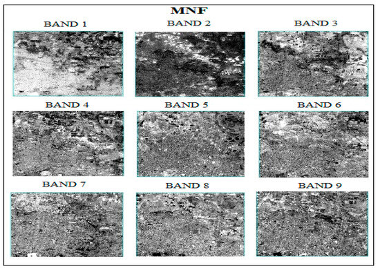
Figure 3.
Minimum noise fraction.
3.2. Interpretation of Eigenvalues Presented ina Scree Plot
The scree test is a criterion used as an optimal method for reducing the dimensionality band from the hyperspectral dataset [6]. From the scree plot, it is shown that the first nine principal components are retained and the bands corresponding to these components provide large data variance when compared with the low-order PC. From the MNF results, it is seen that the first nine eigen images contain coherent information, while the others contain noise. In general, the eigenvalues of the components are decreasing, denoting a lot of available information from a higher to lower order. PCA eigenvalues are larger when compared to MNF, indicating how well the data is spread out in the direction with much variance. However, MNF usually produces higher signal to noise ratios when compared to PCA. Hence, denoising the image is more effective when using the MNF dimensionality reduction transformation. The results were analyzed by incorporating the factor analysis method, in which the acquired components and the total calculated are plotted against a scree graph. The scree graph represents the range of eigenvalues plotted with respect to the principal components as it subsequently tapers towards a lower order, disclosing the noise in the hyperspectral imagery. Eigenvalues with corresponding components for PCA and MNF, along with the generated scree plot, are shown in Table 1 and Table 2, and Figure 4a,b, respectively.

Table 1.
Principal component analysis (PCA) eigenvalue table.
Table 2.
Minimum noise fraction (MNF) eigenvalue table.
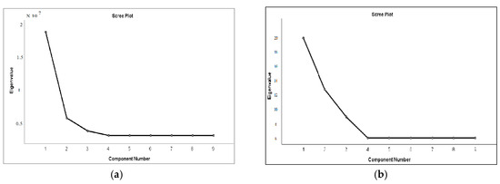
Figure 4.
Scree plot for (a) PCA and (b) MNF.
4. Conclusions
It is concluded from the study that the MNF transform outperforms the PCA dimensionality reduction technique. This is proved through a visual inspection of the resulting gray-scale eigen images and scores provided by the given hyperspectral AVIRIS-NG dataset. The first nine components of the reduced dataset yielding the most information were considered for further analysis.
Author Contributions
Conceptualization and analysis, K.N.P. and V.S.; writing—original draft preparation, K.N.P. and V.S.; review and editing, S.S. and K.B.; supervision, S.S. and K.B.; funding acquisition, S.S.
Funding
This research was carried out under the support of the DST-funded Network Project on Imaging Spectroscopy andApplications (NISA).
Conflicts of Interest
The authors declare no conflict of interest.
References
- Goetz, A.F.H.; Vane, G.; Solomon, E.J.; Rock, B.N. Imaging spectrometry for earth remote sensing. Science 1985, 228, 1147–1153. [Google Scholar] [CrossRef] [PubMed]
- Roger, R.E. Principal components transform with simple, automatic noise adjustment. Int. J. Remote Sens. 1996, 17, 2719–2727. [Google Scholar] [CrossRef]
- Green, A.A.; Berman, M.; Switzer, P.; Craig, M.D. A transformation for ordering multispectral datain terms of image quality with implications for noise removal. IEEE Trans. Geosci. Remote Sens. 1988, 26, 65–74. [Google Scholar] [CrossRef]
- Gao, L.; Zhang, B.; Sun, X.; Li, S.; Du, Q.; Wu, C. Optimized maximum noise fraction for dimensionality reduction of Chinese HJ-1A hyperspectral data. Eurasip J. Adv. Signal Process. 2013, 65. [Google Scholar] [CrossRef]
- Liu, X.; Zhang, B.; Gao, L.; Chen, D. A maximum noise fraction transform with improved noise estimation for hyperspectral images. Sci. China Ser. F: Inf. Sci. 2009, 52, 1578–1587. [Google Scholar] [CrossRef]
- Arslan, O.; AkyÜRek, Ö.; Kaya, Ş. A comparative analysis of classification methods for hyperspectral images generated with conventional dimension reduction methods. Turk. J. Electr. Eng. Comput. Sci. 2017, 25, 58–72. [Google Scholar] [CrossRef]
- Principal Component Analysis. Available online: https://www.harrisgeospatial.com/docs/PrincipalComponentAnalysis.html (accessed on 20 May 2019).
- A Beginner’s Guide to Eigenvectors, Eigenvalues, PCA, Covariance. Available online: https://skymind.ai/wiki/eigenvector (accessed on 20 May 2019).
- Minimum Noise Fraction Transform. Available online: https://www.harrisgeospatial.com/docs/MinimumNoiseFractionTransform.html (accessed on 21 May 2019).
Publisher’s Note: MDPI stays neutral with regard to jurisdictional claims in published maps and institutional affiliations. |
© 2019 by the authors. Licensee MDPI, Basel, Switzerland. This article is an open access article distributed under the terms and conditions of the Creative Commons Attribution (CC BY) license (https://creativecommons.org/licenses/by/4.0/).