Sentinel-1 Data Border Noise Removal and Seamless Synthetic Aperture Radar Mosaic Generation ^†

Abstract

The Canadian Ice Service (CIS, Ottawa, ON, Canada) is receiving hundreds of Synthetic Aperture Radar (SAR) images daily with almost a complete coverage of Canada navigable waters for the monitoring and mapping of seasonal sea and lake ice. In order to efficiently use and analyze such a large amount and wide areal extent of data, short-term (i.e., 12 h to a few days) high-resolution mosaic products are of interest. Among these SAR images, Sentinel-1 data have been known to have an issue of border noise which needs to be removed before generating a seamless mosaic. A method using line-by-line scanning and filtering is proposed, which traces an extreme jump between two neighboring pixels along every scan line. The results show that this method can remove the noise precisely while retaining the rest of the valid data. For visual display, analysis, and interpretation, as done at the CIS, a tone-balanced smooth mosaic is of interest and value to ice analysts in displaying the overall ice distribution and in viewing and comparing cross-region ice conditions. To address this, a scene boundary match balancing method is developed. These short-term mosaic products are proved very helpful in daily ice analysis and macroscopic ice drift measurement.

1. Introduction

The Canadian Ice Service (CIS, Ottawa, ON, Canada) relies on a variety of Earth Observation datasets to operationally monitor sea and lake ice in Canadian waters. Among them, space-borne Synthetic Aperture Radar (SAR) is the primary data source because of its high-resolution, all-weather, and day-or-night collection capability. In addition to RADARSAT-2, recently available Sentinel-1 A and B have provided more capability with enhanced revisit frequency and extended spatial coverage. Currently, a typical 48 h availability of SAR images received at CIS is shown in Figure 1. Considering that the three-satellite RADARSAT Constellation Mission (RCM) developed by the Canadian Space Agency (CSA, Saint-Hubert, QC, Canada) will be launched in late 2018, the number of SAR images will keep increasing without doubt. To help CIS analysts viewing and analyzing data efficiently and comprehensively, automated big data processing and computer-assisted products should be of desirable interest. A regional or Pan-Arctic SAR mosaic product could be one of them. Actually, various SAR mosaic products are developed and used for different applications, such as global forest investigation from L-band ALOS PALSAR [1] and national land mapping from EnviSat ASAR [2]. Unlike land applications where a mosaic may use data collected in a relatively long term, e.g., from one or several months to even a year, sea ice conditions are generally very dynamic and can change dramatically in a few days. Therefore, a short-term (12 h to a few days) and near real-time mosaic for sea ice is required. An automated RADARSAT-2 mosaicking system has been developed before at the CIS [3], and the regional multi-day mosaic images for the Canadian Arctic are provided on a weekly basis [4]. Based on previous works, an improved system is here implemented to be able to incorporate images observed by different satellites and sampled at different scales, such as C-band Sentinel-1, RADARSAT-2, and the future RCM.

It is known that Sentinel-1 images are impacted by the so-called border noise effect. These noises, i.e., non-zero artifacts, appear as a thin strip along the borders of both range and azimuth directions (see Figure 2). They are thought to be caused by processor failure in documenting the invalid sensing areas. Such noise needs to be removed before generating a seamless mosaic. Although the Sentinel Application Platform (SNAP) toolbox [5] released by the European Space Agency (ESA, Paris, France) includes a module called “Sentinel-1 Remove GRD Border Noise”, in practice this tool works well on land but does not work properly over ocean. When the backscattering signals are low, e.g., from water, applying this tool can either leave lots of residuals or take off many valid data. A few other methods have been recently proposed to deal with these noise, and better results are shown comparing to those from the SNAP tool [6,7]. In order to appropriately remove border noises in scenes specifically over sea ice and open water, a method using line-by-line scanning and filtering is proposed in this paper.

2. Mosaic Methodology

The CIS obtains Sentinel-1 A/B Level-1 Ground Range Detected (GRD) products for Canadian waters from the Collaborative Data Hub in Canada (under an agreement between CSA and ESA). The data are processed using a CIS importer, and the output images contain border noises, as shown in Figure 2, where a corner (red box) of a Sentinel-1 scene is enlarged, and the noises are enhanced by a dark blue color. Such border noises should be removed before the data are used for generating a mosaic.

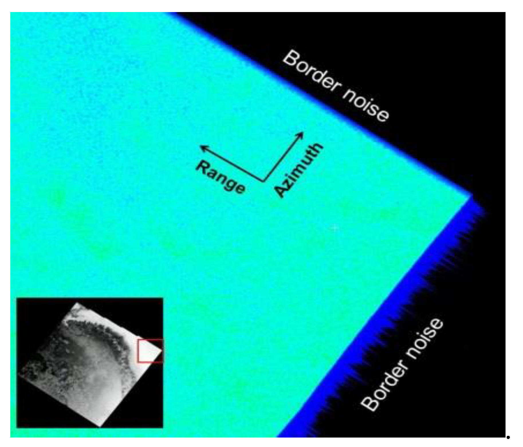
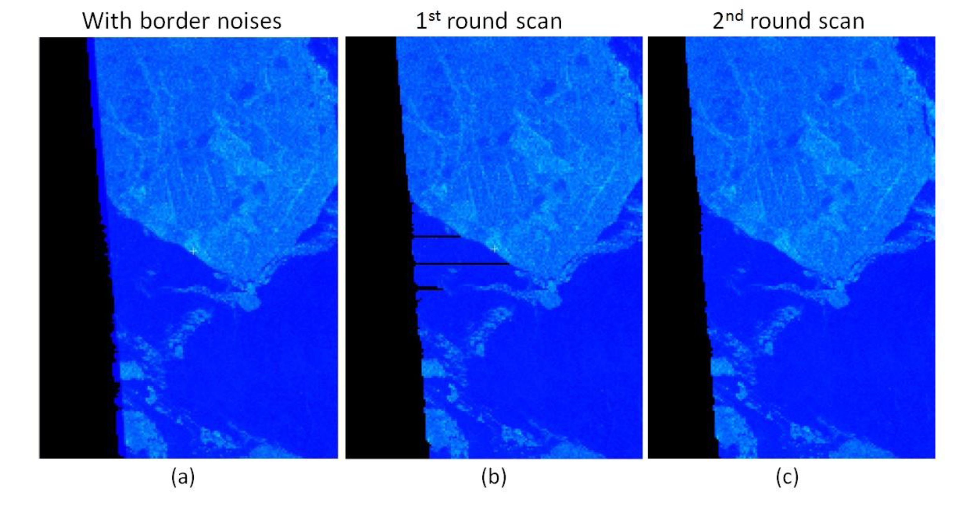
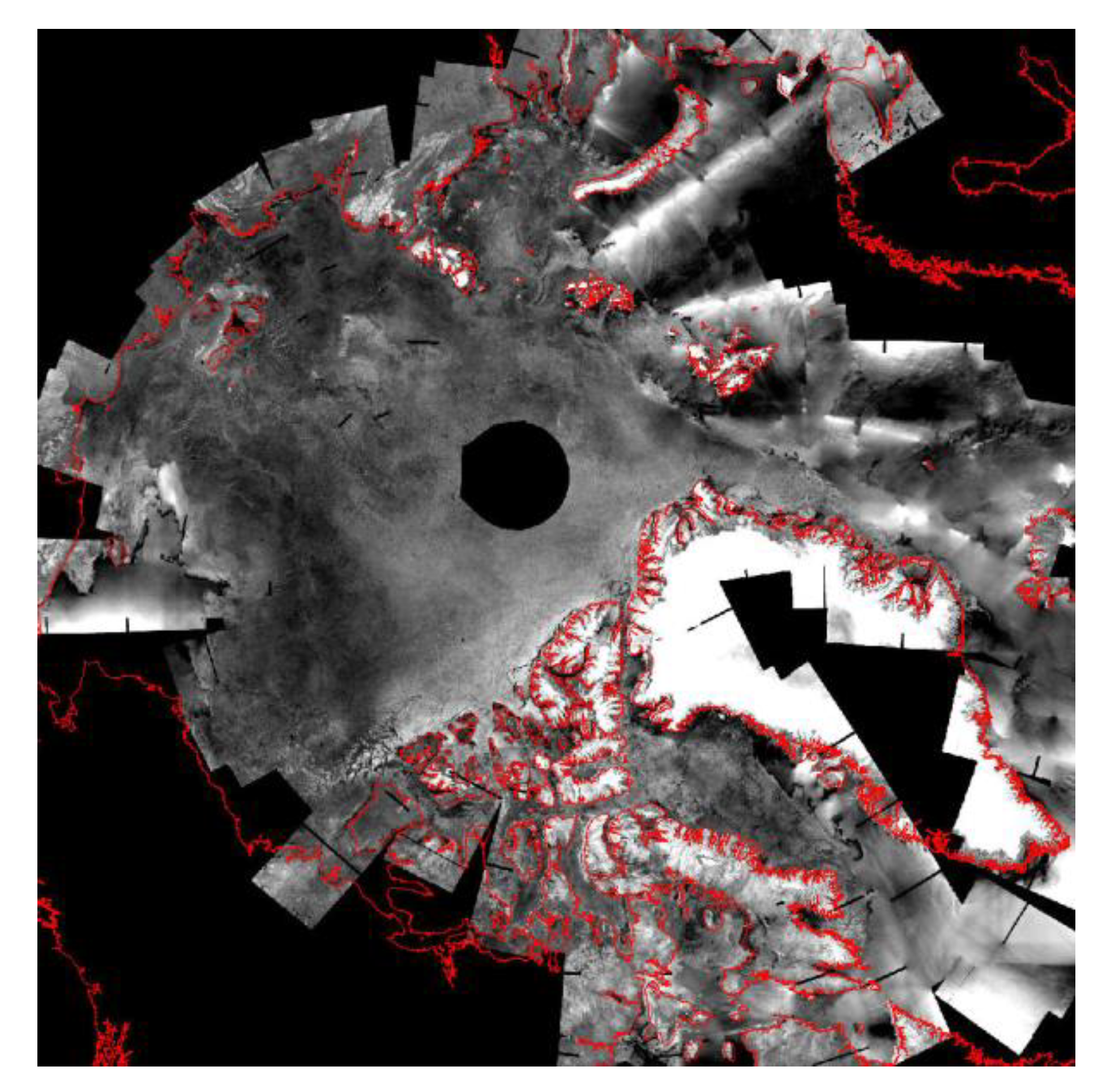
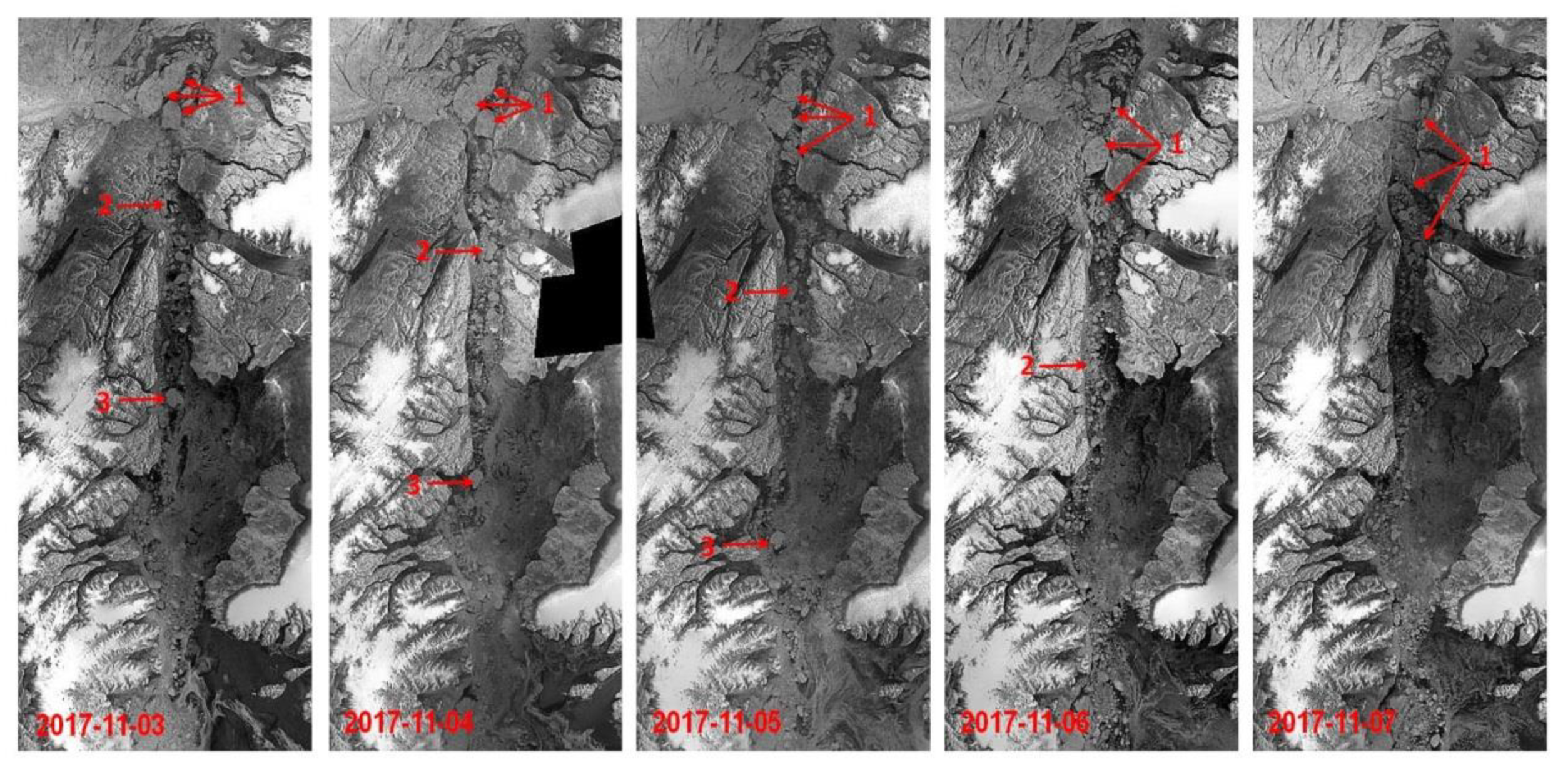
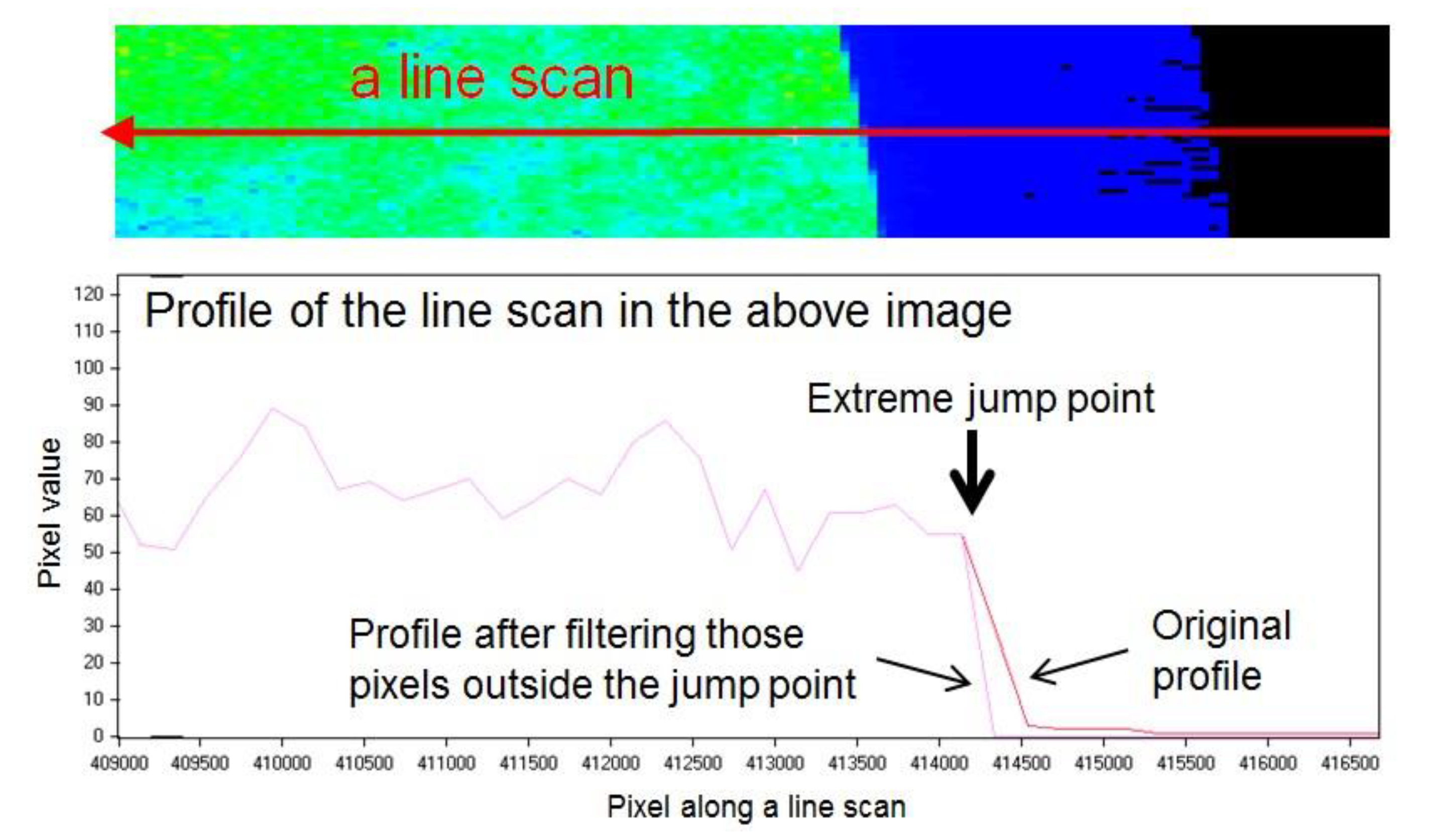
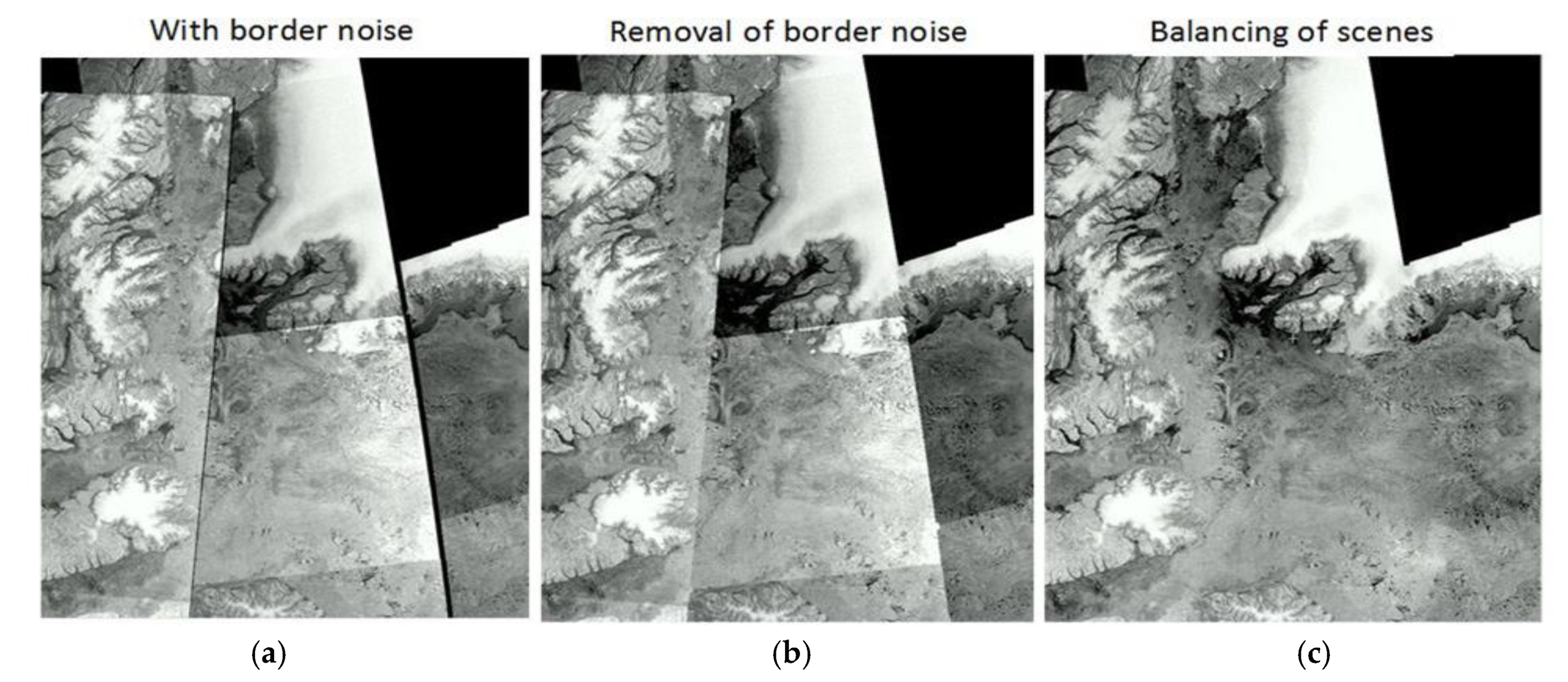
2.1. Border Noise Removal

The magnitude of border noise varies from scene to scene and for a few cases it is even equivalent to that of the valid data, so a predetermined-threshold masking approach is not feasible. Cropping an image by a certain width of border margin may remove the noise but also cut off good data. Such indiscriminate cropping could result in a no-data gap between two consecutive scenes. Considering also that most of the images received are processed already onto a local map projection instead of in their Level-1 swath format, a method using line-by-line scanning and filtering is proposed. The idea is based on the fact that the noise value is generally far lower than a valid value. The method traces an extreme jump between two neighboring pixels along a scan line and then locates the separation point of noise and valid data. The jump can be expressed as a ratio of values of two neighboring pixels (non-zero), and the maximum ratio represents very likely the extreme jump, as displayed in Figure 3. In practice, there is a condition applied to this maximum ratio, i.e., it should be significantly larger than the second maximum ratio. This is to avoid a false locating of the separation point. Generally, this line-by-line scanning and filtering method works for most cases, but there are still a couple of issues, especially for images dominated by open water and sea ice. First, some open water pixels have a very low backscattering that is almost equivalent to those of the noises (see Figure 4a), and then the maximum ratio may not happen at the real separation point but at the boundary of water and ice. This results in an overshot filtering, as shown in Figure 4b. To prevent it, a second round scanning is introduced, which applies a limit on how deep the scanning can get inside the image. The limit depth comes from an average width of noise belt estimated during the first round scanning. The second issue is that, after scanning horizontally and vertically, the noises are not completely removed in some cases, i.e., there are a few noise residuals. To solve it, two additional scans should be done at tilted directions of 45° and 135°, respectively, to the horizontal.

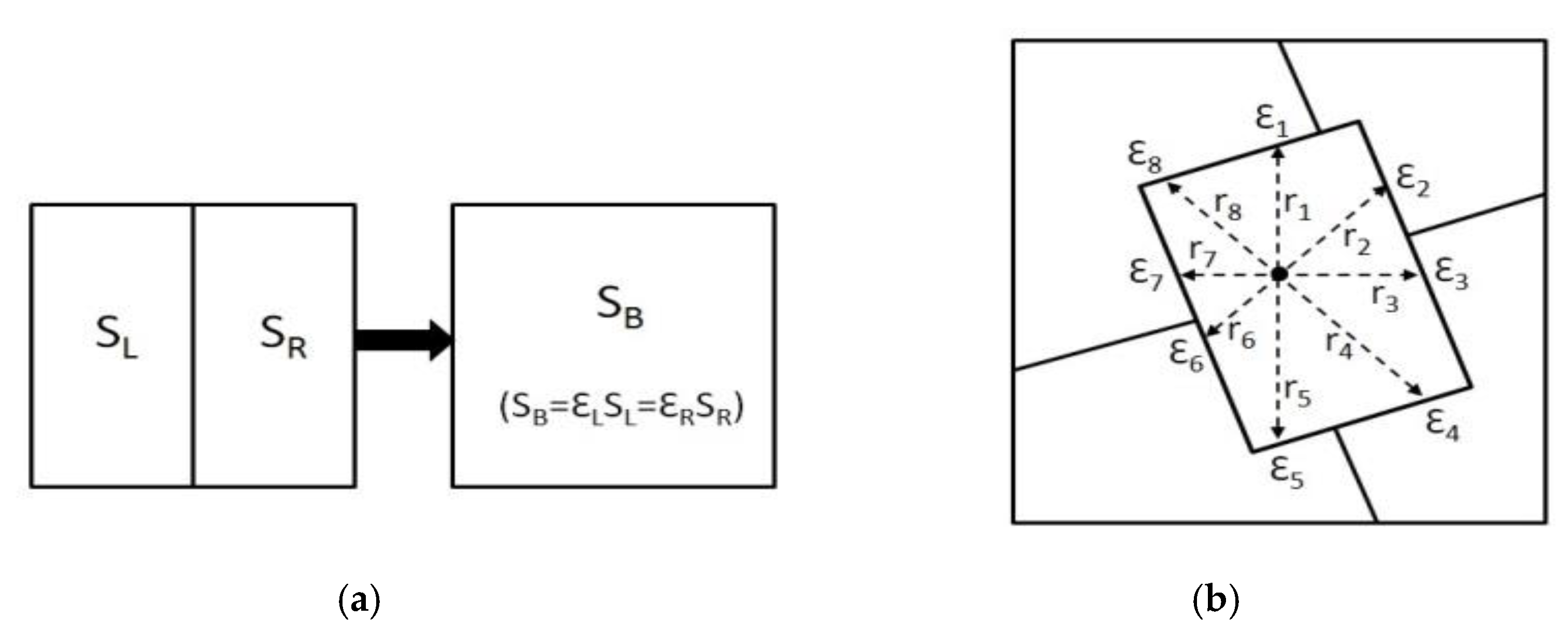
2.2. Tone-Balanced Mosaic Generation

A mosaic is comprised of multiple scenes collected when they fall into an observing time window and a geographic range box. After all scenes are reprojected onto the same map projection (e.g., the polar stereographic one shown in Figure 1) and all pixels are resampled into the same spatial size, they can be stitched together to make one single mosaic image. If there appears overlapping, i.e., more than one scene collected over the same geolocation, only one scene would be retained normally, following a rule suggesting to keep the latest observed or the one with the best quality. Mosaicking SAR images acquired at different times, look directions, and observation angles is a challenge because of the scene-to-scene signal and tonal variations. For visual display, analysis, and interpretation— as it is done at the CIS—a tone-balanced smooth mosaic is of interest and value to ice analysts in displaying the overall ice distribution and in viewing and comparing cross-region ice conditions. To address this, a scene boundary match method is developed to generate a seamless and tone-balanced mosaic product.

Assuming that two scenes have a common boundary, but the boundary values are S_L for the left scene and S_R for the right one, a simple way to match the boundary is to multiply S_L and S_R by the coefficients of ε_L and ε_R, respectively, and then make both sides be equal to a balanced value S_B, as described in Figure 5a. S_B should be thought as a linear or nonlinear combination of S_L and S_R. If it is assumed that there is no difference between S_L and S_R regarding data quality (e.g., signal-to-noise ratio level) or other priorities (e.g., incident angle, weather conditions etc.), S_B = (S_L + S_R)/2 could be a good match. Once the balanced formula S_B is defined, the coefficients ε_L and ε_R could be derived as a function of the boundary values S_L and S_R. Actually, S_L and S_R are not values of a single pixel on the boundary but they are obtained by statistically averaging a bundle of nearby pixels that surround each boundary pixel. For a pixel away from any boundary, the balancing could be impacted by all coefficients of all boundaries. To simplify the process but still efficiently maintain an all-direction balancing scheme, an octal-direction boundary matching is applied, as shown in Figure 5b. The balancing coefficient of any pixel is determined by the sum of eight coefficients (ε₁, ε₂, …, ε₈) weighted by their inverse distance (1/r₁, 1/r₂, …, 1/r₁) which is measured from a boundary to that pixel.

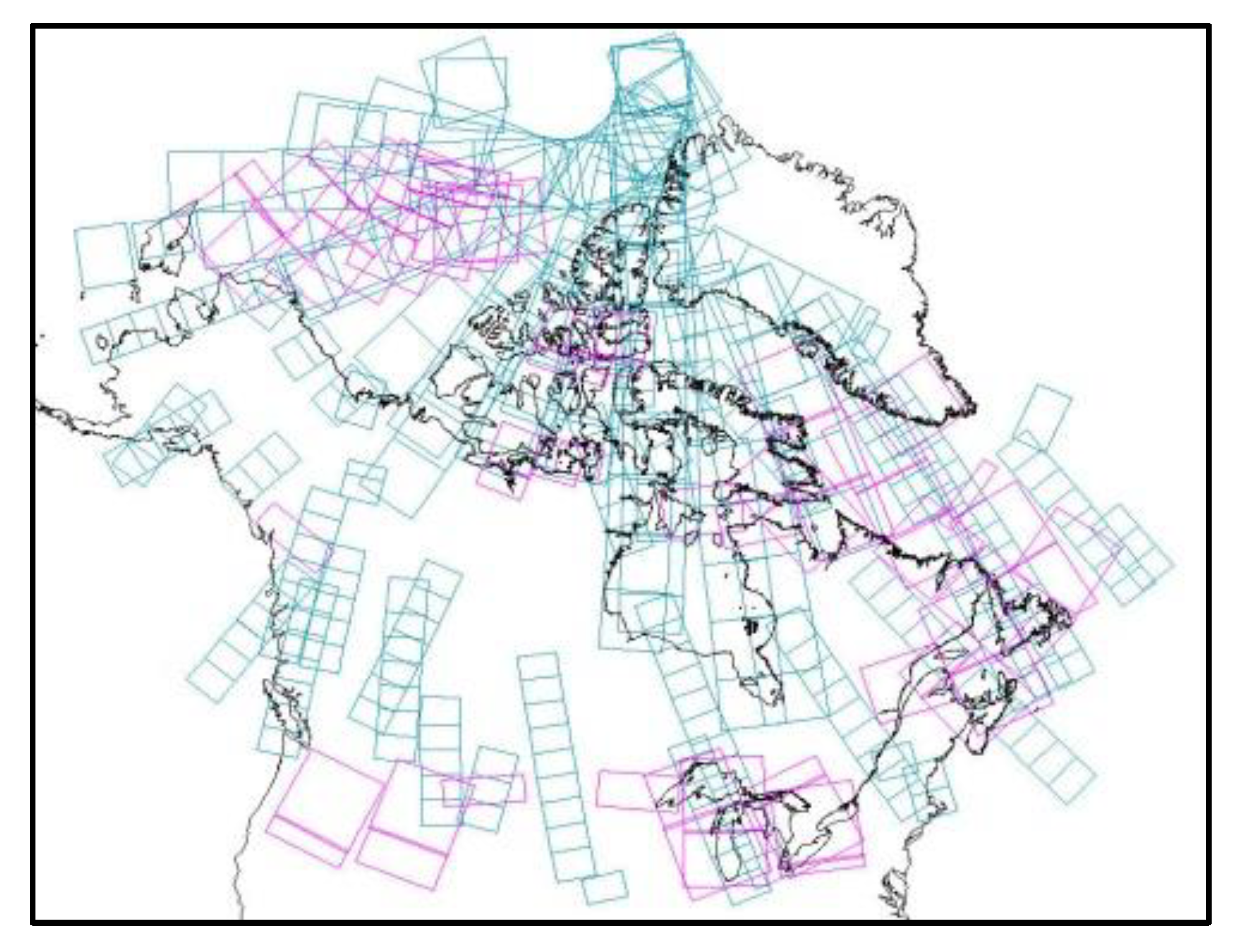
3. Mosaic Results and Applications

The impacts of border noise and tone difference to a mosaic are displayed in Figure 6a, while the results of noise removal and tone balancing are displayed in Figure 6b,c. It is obvious through comparing the three panels in Figure 6 that the methods developed in Section 2 work very well. The dark seams of border noises in Figure 6a are neatly removed in Figure 6b, and then the tone differences in Figure 6b are smoothly balanced in Figure 6c. One of the advantages of the mosaic product is its capability to display an extended coverage at either regional or global scale. For example, by mosaicking as many as 450 Sentinel-1 A/B scenes observed in four days, a Pan-Arctic view of sea ice can be obtained, as shown in Figure 7. Even though it is comprised of hundreds of scenes, the overall balancing process performs quite favorably, especially for the land and sea ice coverage. However, an issue appears over the open water areas (mainly in the upper-right part), where there are still high-contrast tone differences and non-smooth textures. This complexity is caused by the fact that SAR imaging of open water is very sensitive to the radar incident angle as well as local to weather conditions, such as surface wind speed. Another important application of a short-term mosaic product is to trace the ice drift visually or digitally. Five consecutive daily mosaic images over the Nares Strait are provided in Figure 8. To increase the revisit frequency, both Sentinel-1 A/B and RADARSAT-2 data are collected. Three ice targets (Labeled as 1, 2, and 3 in Figure 8) are identified, image by image, and the downward ice movement is traced.

So far, the developed mosaic algorithm and product have been widely used elsewhere, such as in a climatology study reported by the CIS in its “Annual Arctic Ice Atlas” [8] and in an education program initiated by the CSA, entitled “Canada from Space: Giant Floor Map project” [9,10].

4. Concluding Remarks

The border noise removal algorithm of line-by-line scanning has proven to be a feasible and useful tool to improve and perfect the quality of Sentinel-1 data. The seamless and tone-balanced mosaic generation has provided a unique and helpful product for analysts to operationally monitor and analyze sea ice as well as to produce large-scale ice charts. Once more and more SAR data, e.g., the three-satellite RCM, become available, the burden of data collection and the efficiency of data usage could be major concerns for the analysts. A quickly and automatically generated mosaic product with high spatial resolution and extended coverage might be a potential solution. In addition, these short-term mosaic products can also be used as baseline data for further processing where raw data with absolute values are not critical, such as the animation of sea ice change and the quantification of macroscopic ice drift. A large-scale SAR mosaic product can also be used for data fusion with other satellite imagery, e.g., from optical sensors [11], to benefit from particular advantages of different types of data. In order to meet the increasing demand in process automation and in computer-assisted analysis, the current algorithm and product are absolutely helpful, and their continuous improvements are also really necessary.

References

1. Shimada, M.; Itoh, T.; Motohka, T.; Watanabe, M.; Shiraishi, T.; Thapa, R.; Lucas, R. New global forest/non-forest maps from ALOS PALSAR data (2007–2010). Remote Sens. Environ. 2014, 155, 13–31. [Google Scholar] [CrossRef]
2. Zhang, L.; Guo, H.; Liu, G.; Fu, W.; Yan, S.; Song, R.; Ji, P.; Wang, X. SAR China Land Mapping Project: Development, Production and Potential Applications. IOP Conf. Ser. Earth Environ. Sci. 2014, 17, 12229. [Google Scholar] [CrossRef]
3. Luo, Y.; De Abreu, R. Operational RADARSAT-2 Image Mosaicking for the Canadian Arctic. In Proceedings of the 3rd Workshop on RADARSAT-2, Saint-Hubert, QC, Canada, 27 September 2010. [Google Scholar]
4. RADARSAT Mosaics, Canadian Ice Service, Environment and Climate Change Canada. Available online: https://www.canada.ca/en/environment-climate-change/services/ice-forecasts-observations/latest-conditions/products-guides/satellite-images-mosaics-animations.html (accessed on 1 February 2018).
5. Sentinel Application Platform (SNAP), European Space Agency. Available online: http://step.esa.int/main/toolboxes/snap/ (accessed on 1 February 2018).
6. Ali, I.; Cao, S.; Naeimi, V.; Paulik, C.; Wagner, W. Methods to remove the border noise from Sentinel-1 Synthetic Aperture Radar data: Implications and importance for time-series analysis. IEEE J. Sel. Top. Appl. Earth Obs. Remote Sens. 2018, 99, 1–10. [Google Scholar] [CrossRef]
7. Dyatmika, H.S.; Sambodo, K.A.; Budiono, M.E.; Hendayani. Noise removal using thresholding and segmentation for random noise Sentinel-1 data. IOP Conf. Ser. Earth Environ. Sci. 2017, 54. [Google Scholar] [CrossRef]
8. Annual Arctic Ice Atlas: Winter 2015–2016, Canadian Ice Service. Available online: https://www.canada.ca/en/environment-climate-change/services/ice-forecasts-observations/publications/annual-arctic-atlas-winter-2015-2016.html (accessed on 1 February 2018).
9. Canada from Space, Canadian Space Agency. Available online: http://www.asc-csa.gc.ca/eng/search/images/watch.asp?id=2572 (accessed on 1 February 2018).
10. Giant Floor Map: Canada from Space, Canadian Geographic Education. Available online: http://www.canadiangeographic.com/educational_products/canada_from_space_map.asp (accessed on 1 February 2018).
11. Luo, Y.; De Abreu, R. Data fusion of RADARSAT and MODIS images for Arctic sea ice mapping. In Proceedings of the American Meteorological Society Annual Meeting, Seattle, WA, USA, 22–27 January 2011. [Google Scholar]
Figure 1. Availability of Synthetic Aperture Radar (SAR) images at the Canadian Ice Service (CIS) during 6 and 7 February 2018, for RADARSAT-2 (pink) and Sentinel-1 A/B (blue).
Proceedings 02 00330 g001
Figure 2. Border noises in Sentinel-1 image that appear along both the range and the azimuth edges.
Proceedings 02 00330 g002
Figure 3. Diagram of a line scan and profile of the line scan.
Proceedings 02 00330 g003
Figure 4. (a) Sentinel-1 image with border noises on the left edge; (b) first-round scan with noises removed, but a few overshooting lines; (c) second-round scan by a limited width of noise belt estimated through the first-round scan.
Proceedings 02 00330 g004
Figure 5. (a) Balancing at boundary by matching two scenes’ boundary pixels; (b) rebalancing for any pixel within a scene through octal-direction-weighted boundary matching.
Proceedings 02 00330 g005
Figure 6. An example of Sentinel-1 mosaic. (a) Mosaic without border noise removal; (b) mosaic after noise removal; (c) mosaic with tone balancing.
Proceedings 02 00330 g006
Figure 7. Mosaic of Sentinel-1 A/B. A total of 450 scenes that were acquired between 18 and 21 Novemebr 2017 are used.
Proceedings 02 00330 g007
Figure 8. Daily mosaic of combined Sentinel-1 A/B and RADARSAT-2 over the Nares Strait.
Proceedings 02 00330 g008
Publisher’s Note: MDPI stays neutral with regard to jurisdictional claims in published maps and institutional affiliations.