Abstract
Spatial localization of emitting sources is especially interesting in different fields of application. The focus of an earthquake, the determination of cracks in solid structures or the position of bones inside a body are some examples of the use of multilateration techniques applied to acoustic and vibratory signals. Radar, GPS and wireless sensors networks location are based on radiofrequency emissions and the techniques are the same as in the case of acoustic emissions. This paper is focused on the determination of the position of sources of partial discharges inside electrical insulation for maintenance based on the condition of the electrical machine. The use of this phenomenon is a mere example of the capabilities of the proposed method because its emission can be electromagnetic in the UHF range or acoustic when the insulation is immersed in oil. Generally, when a pulse is radiated from a source, the wave will arrive to two receivers at different times. One of the advantages of measuring these time differences of arrival or TDOA is that it is not required a common clock as in other localization techniques based on the time of arrival (TOA) of the pulse to the receiver. With only two sensors, all the possible points in the plane that would give the same TDOA describe a hyperbola. Using an independent third receiver and calculating the intersection of the three hyperbolas will give the position of the source. Therefore, planar localization of emitters using multilateration techniques can be solved at least with three receivers. This paper presents a method to locate sources in a plane with only two receivers, one of them in a fixed position and the other is placed describing a circumference around the first one. The TDOA are measured at different angles completing a total turn and obtaining a function, angle versus TDOA, that has all the geometric information needed to locate the source. The paper will show how to derive this function analytically with two unknown parameters: the distance and bearing angle from the fixed receiver to the source. Then, it will be demonstrated that it is possible to fit the curve with experimental measurements of the TDOA to obtain the parameters of the position of the source.
1. Introduction
The localization of emitting sources is an interesting research topic which covers several fields, from earthquake detection, to RADAR and GPS applications. All of them can use multilateration techniques applied to radio-frequency, acoustic and vibration signals which are acquired with several fixed sensors. Generally, the time differences of arrival (TDOA) between these sensors are used as input variables in a non-linear equation system for the localization of the source. Depending on the type of sensor and application, between 3 and 4 receivers are needed for 2D or 3D localization, respectively.
In this paper, the authors face the problem from a different point of view moving at least one of the receivers with the aim of reducing the number of sensors using the known position of their relative movement to obtain the needed TDOA for the localization of pulsed sources.
In this work, the pulsed source will be a phenomenon known as partial discharges (PD) which are small-energy ionizations taking place within insulation materials revealing accelerated ageing. It is well known that the detection of PD can be used to prevent premature failures of power cables and electric machines [1]. In the particular case of open-air substations, the radio-frequency (RF) radiation emitted by PD can be used to detect and locate the imperfections, giving valuable information for condition monitoring [2]. Typically, the localization of PD sources using RF signals has been done through a system of 4 omnidirectional antennas [3]. The position of the receivers and TDOA of the pulses arriving to these sensors form a system of non-linear equations that can be solved to locate the emitter [4]. However, in the RF range the sampling frequencies ought to be high to have sufficient resolution so the acquisition systems have fairly high costs. Thus, a reduction in the number of receivers could help in the reduction of the price of the instrumentation (sensors, channels of the acquisition system …). Therefore, the authors propose a system for planar localization of PD sources by means of two sensors mechanically linked by a rod. In order to get the necessary number of different TDOA for the localization (with one value it is impossible), one of the sensors is moved (rotated) fixing the other one as a geometric reference. The mathematical function relating the relative distance between the two sensors, the rotation angle of the moveable one, and the TDOA will be derived in the paper showing good agreement with the experimental results. It will also be shown that the localization can be successful done using only these two sensors. The results obtained here are not restricted to this type of pulsed source, since the same strategy could be applied to other type of signals whose source needed to be localized.
2. Basis
The proposed method is based on the information of the arrival of pulsed signals to two sensors, in this case, two simple omnidirectional antennas, as a function of their relative position with respect to the source. The TOA from the source to the antenna i, , is not known since the position of the source has not yet been determined. Therefore, the localization relies on the time differences of arrival, of the emission to the antennas as in all multilateration techniques. The novelty of this work is presented henceforth. The distance between antennas is fixed attaching them to the ends of a shaft or rod. Then, both antennas can be moved jointly when the rig is rotated around the vertical axis passing through the middle point between the antennas or the antenna 1 (▲) can be fixed at the origin of a cartesian coordinate system while the antenna 2 (▼) rotates around the antenna 1 as shown in Figure 1 where the source (●) is placed at m. Though both possibilities are valid, the latter configuration is preferable to moving both antennas simultaneously since one of the receivers is always placed in the same site.
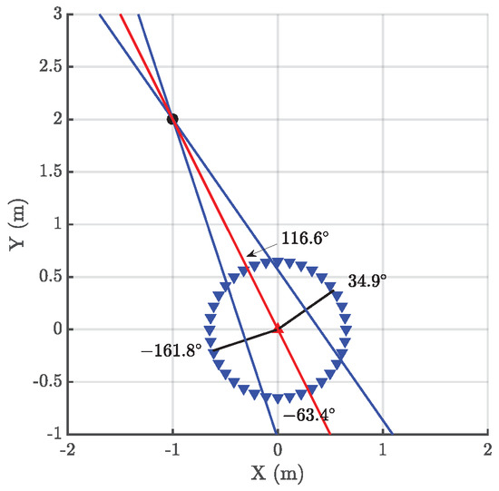
Figure 1.
Different positions represented of antenna 2 marked with triangles (▼) when turned around the fixed antenna 1 (▲).
2.1. Intersection of lines
The process consists on measuring the TDOA at different angles completing a total turn to obtain the theoretical function plotted in Figure 2. The units of the TDOA are usually seconds but they can also be represented in meters multiplying time by the speed of light c, or samples, dividing time by the sampling time . The choice of samples for the plot in the figure is to bear in mind that the sampling frequency and the length of the rod are related and affect the sensibility as will be explained in Section 2.3.
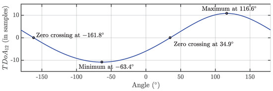
Figure 2.
Periodic function representing the TDOA vs the rotating angle. The units in the TDOA are samples because it is easier to study the sensibility of the rig.
There are two possible methods to determine the position of the source. One of them is based on the intersection of two lines perpendicular to the rod when and the other is based on the determination of the analytical expression of the periodic function in Figure 2 and fitting the curve to the experimental data. These two procedures are explained in the next sections.
There are four characteristic points in the periodic function: two zero crossings, and maximum and minimum values. The maximum corresponds to one of the maxima TDOA which occurs when the rod is aligned with the direction of the source, therefore, antenna 1, antenna 2 and source are in the same line. Figure 1 shows this particular case when the antenna 2 is placed at , then and . There is also a minimum at the opposite angle, , because there are two positions where the three elements are aligned. In this case, the relative locations of antenna 1 and antenna 2 are swapped and the TDOA is negative, and . The function also crosses zero twice and this happens when the rod is perpendicular to the direction of the source because, in that case, both times of arrival to the antennas are the same, and , black radii in Figure 1. These cases are more helpful because plotting the perpendicular lines at the angular positions defined by the two zero crossings and calculating the intersection of the two lines will determine and solve the position of the source. Figure 1 shows these locations at and and the lines perpendicular to the rod that intersect at the source.
In summary, the procedure to determine the position of the source is straightforward. First, the TDOA at different angles in one turn are calculated analysing the onset of the pulses of the incoming signals to both antennas using any algorithm presented in [5] which, in this work, is based on the Hinkley criterion. Then, the angles where the TDOA are minima, and , are calculated interpolating the closest angles above and below zero. The next step traces the line perpendicular to the rod at those angles passing through its middle point. Finally, the position of the source is calculated with the intersection of those lines.
2.2. Analytical Expression of the Periodic Function
The analytical expression of the periodic function defined in Figure 2 can be derived from the setup in Figure 3 where is the distance from the antenna i to the source. The antenna 1 is located at the origin of coordinates and the positions of the source and the antenna 2 are defined by their radius and azimuth in cylindrical coordinates and , respectively. The TDOA in meters can be calculated subtracting the distances, , which is better done in cartesian coordinates:
where are the coordinates of the source, the position of the antenna 2 and r the constant distance between antennas. Therefore, is calculated as:
or, rearranging the terms, as:
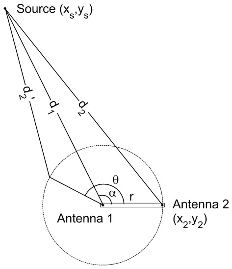
Figure 3.
Source and antenna positions to determine the analytic expression of the periodic function vs TDOA.
Equation (3) depends on the position of the source, determined by and ; the distance between antennas, r and the rotation angle, . The only unknown parameters are and , so fitting the experimental data to the analytical expression with a non-linear least squares algorithm will determine these parameters and, therefore, the position of the source.
2.3. Choosing the Separation Distance
The separation between antennas is a critical parameter that will determine the accuracy of the calculated position of the source. The maximum time difference of arrival can be derived from Equation (3) considering that , or . In that case, the square root would be minimum and the maximum TDOA in meters would be:
This result is expected since when the antennas are aligned (), the relative distance between the antennas and the source would be maximum and equal to the distance between them, r. This parameter is directly related to the sampling frequency and the sensibility of the rig. In effect, since the sampling time determines the minimum measurable distance, the minimum step of would be one sample or meters. We have considered that it would be necessary to have at least ten steps in the maxima of the curve in Figure 2 to reach a sufficiently high resolution, therefore, or . This figure of merit would ensure that the zero crossings can be determined with good accuracy.
3. Analysis of the measurements
The TDOA for 500 pulses, obtained subtracting the onsets determined with the Hinkley criterion, are plotted versus the angle of rotation in a box plot in Figure 4. The bottom and top of the boxes in blue represent the boundaries for 25 % to 75 % of all the values obtained for the TDOA while the red line inside the box represent the median value. The red crosses outside the box are estimations of the TDOA given by the algorithm for some of the pulses that have not clear onsets. These cases give TDOA outside the boundaries of the box so they can be considered statistical outliers though they are also considered in the calculation of the median value and the boundaries of the box. Admitting that it may be thought that the number of outliers is high, it can be clearly seen that the boxes are very narrow which means that most of the results are concentrated around the median. Figure 5 shows the fitting of periodic function considering only the median of all TDOA in every angle of rotation. The numerical results after the fitting are m and while the exact values, considering the layout in Figure 1 are m and which are very close to the estimated position. The shift between the source and the estimated position is cm mostly due to the difference in the distance because the error in the angle is only . The mean square error of the fitting considering the median of the TDOA is also very low samples. The estimated zero crossings obtained with the method presented in Section 2.1 are and which are very close to the theoretical ones in Figure 2. Though the error is well below in both angles, the intersection of the lines falls far from the actual position of the source: m and m. It is very common, when localizing sources, that the error in the bearing angle is low while the error in the distance is high.
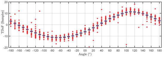
Figure 4.
Box plot of the time differences of arrival versus angle of rotation for the pulses generated by the pulsed source.
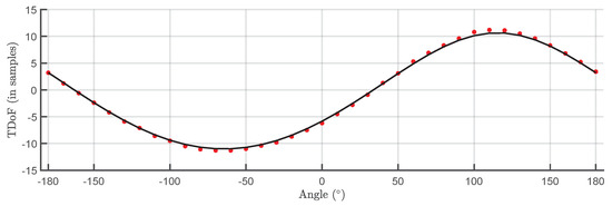
Figure 5.
Median of all TDOA versus rotation angle.
4. Conclusions
The method that fits the derived function to experimental data has been successfully tested obtaining low errors in the localization of the source. Though the accuracy is pretty high, it can be further improved filtering the incoming signals with denoising techniques based in the wavelet transform, for instance. The method based on the intersection of lines gives two angles where the TDOA is zero with high accuracy. Unfortunately, small errors in these angles yields high errors in the estimated position of the source.
Acknowledgments
The work done in this paper has been funded by the Spanish Government under contract DPI2015-66478-C2-1-R (MINECO/FEDER, UE).
References
- Stone, G.C.; Warren, V. Effect of manufacturer, winding age and insulation type on stator winding partial discharge levels. IEEE Electr. Insul. Mag. 2004, 20, 13–17. [Google Scholar] [CrossRef]
- Moore, P.J.; Portugues, I.E.; Glover, I.A. Radiometric location of partial discharge sources on energized high-voltage plant. IEEE Trans. Power Deliv. 2005, 20, 2264–2272. [Google Scholar] [CrossRef]
- Markalous, S.M.; Tenbohlen, S.; Feser, K. Detection and location of partial discharges in power transformers using acoustic and electromagnetic signals. IEEE Trans. Dielectr. Electr. Insul. 2008, 15. [Google Scholar] [CrossRef]
- Robles, G.; Fresno, J.M.; Sánchez-Fernández, M.; Martínez-Tarifa, J.M. Antenna Deployment for the Localization of Partial Discharges in Open-Air Substations. Sensors 2016, 16, 541. [Google Scholar] [CrossRef] [PubMed]
- Robles, G.; Fresno, J.M.; Giannetti, R. Ultrasonic bone localization algorithm based on time-series cumulative kurtosis. ISA Trans. 2017, 66, 469–475. [Google Scholar] [CrossRef] [PubMed]
Publisher’s Note: MDPI stays neutral with regard to jurisdictional claims in published maps and institutional affiliations. |
© 2018 by the authors. Licensee MDPI, Basel, Switzerland. This article is an open access article distributed under the terms and conditions of the Creative Commons Attribution (CC BY) license (https://creativecommons.org/licenses/by/4.0/).