Abstract
In Spain, several major cities face high rates of avoidable deaths due to NO2 exposure. Understanding NO2 atmospheric dynamics is essential to support public health efforts and policymaking. Recent satellite products have proven useful in characterizing urban atmospheric composition in various regions. This study compares NO2 concentration data from in situ air quality monitoring networks and the Sentinel-5P TROPOMI satellite in Spain’s three largest cities (Madrid, Barcelona, and Valencia), alongside O3 levels —due to its close photochemical relationship with NOx—wind speed and direction, temperature, relative humidity, and solar radiation. Data from 2022 were analyzed using Pearson correlation coefficients and Principal Component Analysis (PCA) to identify key relationships and patterns. Results showed a consistent negative correlation between NO2 and O3, wind speed, temperature, and solar radiation. Differences between in situ and satellite data were more pronounced in coastal cities, influenced by wind patterns and urban morphology (Madrid: r = 0.86, v = 1.34 m/s; Valencia: r = 0.68, v = 2.97 m/s; Barcelona: r = 0.65, v = 8.04 m/s). These insights enhance the understanding of NO2 behavior in urban environments and support the use of remote sensing to estimate surface-level pollution in areas lacking ground-based monitoring infrastructure. This is the first study in Spain to jointly evaluate NO2 from satellite and in situ data across multiple cities, linking pollutant concentrations with meteorological and chemical drivers to improve surface-level estimation strategies and support air quality assessment in under-monitored areas.
1. Introduction
When assessing air quality, nitrogen oxides (NOx), which encompass nitrogen monoxide (NO) and nitrogen dioxide (NO2), emerge as undisputed protagonists with a multifaceted impact. These compounds, resulting from the combination of oxygen and nitrogen at high temperatures, can originate naturally (e.g., lightning, volcanic eruptions, biomass burning) [1,2], but their persistence in urban environments stems from the intensive development of activities involving the combustion of fossil fuels (e.g., road transportation, power generation, domestic heating) [3]. Therefore, NO2 concentration tends to grow with population density.
Once emitted, NOx rapidly transforms into NO2, which can have harmful effects on human health by causing diseases of the immune, circulatory, and respiratory systems [4]; on ecosystems, by triggering processes of acidification and eutrophication [5]; and on historical heritage, by accelerating the corrosion of buildings and monuments [6]. It can further react with other substances and generate secondary pollutants, mainly particulate matter, nitric acid (HNO3), peroxyacetyl nitrates (PANs), and tropospheric ozone (O3).
Increasing NO2 pollution in urban environments raises global concern, as 70% of the world’s population will live in cities by 2050 [7]. The European Union has long aimed to tackle this issue. According to current regulations, the annual NO2 limit value is 40 µg/m3. However, plans are underway to halve this threshold in the near future, with the ultimate goal of eventually meeting the World Health Organization (WHO) recommendation of 10 µg/m3 [8]. In Spain, these efforts involve updating legal frameworks, which advocate for the establishment of low-emission zones in municipalities with over 50,000 inhabitants, and the adoption of more efficient and sustainable transportation models. Yet, Spanish major cities have been identified as some with the highest number of avoidable deaths due to NO2 in Europe, with Madrid ranking 1st, Barcelona 6th, and Valencia 68th [9]. Out of the 130 air quality zones designated in Spain in 2022, 30 did not meet the annual limits for NO2 projected by the European Union, and 84 did not meet those recommended by the WHO.
To ensure the ongoing monitoring of air quality and assess the efficacy of new policies, data on pollution levels are gathered via in situ stations. However, in recent years, remote sensing has become an increasingly valuable tool for air quality monitoring, offering spatially continuous data that complement the limited coverage of in situ networks. Satellite-based instruments have been used not only to estimate pollutant concentrations, but also to assess the effectiveness of environmental policies, model emission inventories, and identify pollution hotspots across diverse regions [10,11,12,13]. Among the most commonly used sensors for tropospheric NO2 monitoring are the Ozone Monitoring Instrument (OMI), the Global Ozone Monitoring Experiment–2 (GOME-2), and the TROPOspheric Monitoring Instrument (TROPOMI), which is onboard the Sentinel-5 Precursor satellite. TROPOMI represents a major step forward due to its enhanced spatial resolution (3.5 × 5.5 km2 since 2019) and daily global coverage, making it particularly suitable for detecting urban-scale NO2 variability [14,15].
Despite these advances, the accuracy of satellite-derived NO2 measurements is influenced by several factors. Retrieval algorithms estimate vertical column densities based on radiative transfer models, which are sensitive to aerosol presence, cloud cover, surface reflectivity, and solar zenith angle [16]. Data may be excluded or flagged under unfavorable conditions, such as high cloud fraction and low-quality pixels, and tropospheric NO2 can be underestimated in coastal or topographically complex environments due to mixing layer variability and vertical stratification [17,18]. Furthermore, the resolution of satellite data, while improving, still limits the ability to resolve local gradients and street-level pollution peaks captured by ground-based stations. Nevertheless, multiple studies have shown strong correlations between TROPOMI-derived NO2 values and in situ observations in urban contexts [10,13,17,19,20,21,22], confirming its potential for supporting air quality assessments and policymaking strategies in areas lacking dense monitoring infrastructure.
However, the strength of the correlation between satellite and ground-based NO2 measurements can vary substantially depending on local conditions. To improve surface-level NO2 estimations in areas where satellite performance is less consistent, it is essential to understand the environmental drivers that influence this relationship. Yet, most studies often neglect how local meteorological and geographical conditions may influence the reliability of satellite-derived NO2 estimations. Climatic, meteorological, and geographical factors affect the distribution and detectability of NO2, both directly (e.g., dispersion, removal, chemical conversion, changes in mean lifetime) [23,24,25,26,27] and indirectly (e.g., boundary layer height) [28,29,30]. As a result, relying solely on satellite data to estimate surface-level NO2 concentrations may be insufficient in certain urban settings, unless these local dynamics are properly considered [31,32,33].
Few studies have aimed to address this gap, which is particularly relevant in countries like Spain, where urban NO2 pollution is a major concern. This study provides an updated assessment of NO2 remote sensing performance across three major Spanish cities—Madrid, Barcelona, and Valencia—with distinct meteorological and geographical characteristics. It integrates all available meteorological and air quality data from 2022 and examines their relationship with NO2 concentrations derived from both ground-based monitoring networks and Sentinel-5P satellite observations. In addition, surface-level O3 concentration is incorporated due to its strong involvement in NOx conversion processes. This is the first study to conduct this type of comparative analysis using both in situ and satellite data across multiple cities.
The objective is to improve understanding of air quality dynamics in these locations and to explore the feasibility of using satellite data to estimate surface-level NO2, particularly in municipalities lacking robust air quality monitoring infrastructure.
2. Materials and Methods
2.1. Regions of Interest and Study Period
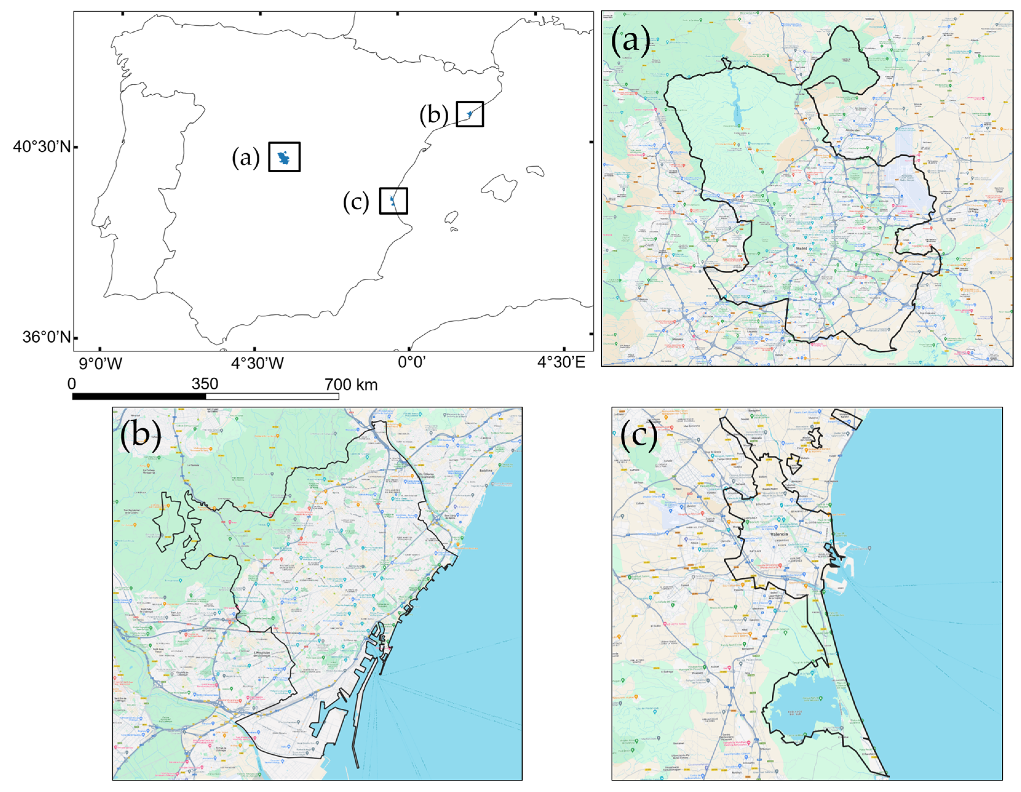
The study regions were the cities of Madrid (3,332,035 inhabitants, Figure 1a), Barcelona (1,660,122, Figure 1b), and Valencia (807,693, Figure 1c) [34]. The study covered the period from 1 January to 31 December 2022.

Figure 1.
Geographical location of the cities of (a) Madrid, (b) Barcelona, and (c) Valencia in Spain.
2.2. In Situ Data
Surface-level NO2, O3, and all meteorological variables information were obtained from the monitoring stations networks located within the city boundaries. Hourly NO2 and O3 concentrations are typically measured by chemiluminescence analyzers and ultraviolet photometry devices, respectively, and provide data in mixing ratio units (µg/m3). Hourly wind speed (m/s), wind direction (°), temperature (°C), relative humidity (%), and solar radiation (W/m2) data were simultaneously available in all three cities. Wind direction data, which can be heavily influenced by the sampling location in urban environments [35,36] were instead derived from the ERA5-Land hourly model [37], in line with previous research [12,38]. The geographical location of the stations is presented in Figure S1, and data availability is shown in detail in Table S1.
All this information was openly available in all cases [39,40,41,42,43].
2.3. Satellite NO2 Data
TROPOMI, developed jointly by the European Space Agency (ESA) and the Netherlands Space Office, is the sensor aboard the Copernicus Sentinel-5P satellite. Launched into orbit in September 2017, its mission is to monitor atmospheric composition and air quality until the future launches of Sentinel-4 [44] and Sentinel-5 [45]. With its capability to measure in the UV (270–500 nm), NIR (675–775 nm) and SWIR (2305–2385 nm) bands, TROPOMI facilitates the observation of a wide range of atmospheric pollutants [46]. Since June 2018, it has provided openly available daily global imagery, initially at a resolution of 3.5 × 7.5 km2, which was subsequently enhanced to 3.5 × 5.5 km2 in August 2019. Sentinel-5P operates on a near-polar, sun-synchronous orbit at an altitude of 824 km. It completes 14 orbits per day, with an ascending node equatorial crossing at 13:30 Mean Local Solar Time [15]. In Madrid, Barcelona, and Valencia (UTC + 1 in winter; UTC + 2 in summer), Sentinel-5P overpasses consistently occurred between 12 PM and 4 PM (local time) in 2022. Occasionally, two consecutive orbits may overlap in some regions, resulting in two readings with a 100 min difference in the same day.
The ESA classifies TROPOMI products into three categories based on the processing level: Level-0, Level-1, and Level-2 [47]. Level-2 images include information on aerosol layer height, absorbing aerosol index, and geolocated total columns of carbon monoxide (CO), sulfur dioxide (SO2), methane (CH4), formaldehyde (CH2O), ozone (O3), and NO2. These are primarily derived from a DOAS algorithm, similar to other satellite missions [16,48]. For NO2, two types of column products are available: the total vertical column and the tropospheric vertical column. In this study, we used the tropospheric column retrievals from the offline (OFFL) processing chain, which offers higher quality and improved post-processing compared to the near-real-time (NRTI) products, albeit with a longer data delivery time.
In previous studies that worked with TROPOMI images and air quality station data simultaneously, additional processing of the images was performed, obtaining Level-3 products [10,19]. The Level-3 images used in this paper stem from Level-2 products that were further processed using the harp-converter drive tool with the bin-spatial operation, obtaining an orthorectified raster layer in a 0.01 × 0.01 degrees resolution mosaic. High cloud cover, low-quality pixels (<75%), and vertical column density values below −0.001 mol/m2 were masked, following the data provider recommendations [49]. Original mol/m2 units were converted to Dobson units (DU).
2.4. Data Processing
The study employed a multi-step statistical approach to explore the relationship between NO2 concentrations and environmental variables. First, the temporal evolution of pollutant and meteorological data was assessed using 30-day moving averages to smooth short-term fluctuations. Pearson correlation coefficients were then calculated to evaluate linear associations between variables. To complement this, extreme pollution events were identified by isolating the upper and lower 10% of NO2 values, allowing for comparative analysis of meteorological conditions under different pollution regimes. Finally, Principal Component Analysis (PCA) was used to reduce dimensionality and detect underlying structures among the variables, offering a synthetic view of the dominant patterns influencing air quality in each city [50]. The analysis included NO2 concentrations (from both in situ and satellite sources), O3, wind speed and direction, temperature, relative humidity, and solar radiation. A PCA was performed using statistical software with built-in multivariate analysis functions [51], following standard procedures for component extraction based on the Kaiser criterion (eigenvalues > 1) and scree plot interpretation.
To enable a direct comparison between both NO2 datasets, satellite observations were obtained at the precise locations of each air quality monitoring station. Following a similar approach to previous studies [22,52], regional daily values were calculated by averaging data falling between Sentinel-5P overpass times (12 p.m. to 4 p.m.) and removing outliers using a 3σ (standard deviation) limit. Scalar averaging was applied for NO2 and O3 concentrations, temperature, relative humidity, and solar radiation, while vector averaging was performed for wind speed and wind direction. The temporal evolution of all variables was represented using 30-day moving averages.
Given the heavy influence of wind on the transport of atmospheric pollution, monthly tropospheric NO2 spatial distributions observed by TROPOMI were compared with wind speed (measured by the meteorological stations) and wind direction (derived from the ERA5 model) data.
3. Results
3.1. Data Overview
Table 1 presents the key statistics of all variables in each city. A daily record was available for each dataset, except for the TROPOMI images, which did not always meet quality criteria. NO2 data from ground stations placed Madrid as the city with the highest pollution levels, with concentrations 1.4% higher than those in Barcelona and 22.2% higher than those in Valencia. In the case of TROPOMI observations, the differences were 12.8% and 61.8%, respectively.

Table 1.
Statistical summary of the study variables.
O3 concentration values were similar in all three cities, with Madrid presenting the highest average level (72.8 µg/m3), followed by Valencia (72.2 µg/m3) and Barcelona (68 µg/m3). However, the differences between maximum values were larger, being 147 µg/m3 in Madrid, 129 µg/m3 in Barcelona, and 113 µg/m3 in Valencia.
The highest average wind speed was recorded in Barcelona (8.04 m/s), as were both extreme values (2.15 m/s and 29.6 m/s). The highest average temperature was observed in Valencia (22 °C), while the annual minimum (6.3 °C) and maximum (37.8 °C) occurred in Madrid. The highest average solar radiation (595 W/m2) and extreme values (49.3 W/m2 and 977 W/m2) were also recorded in the capital. Mean relative humidity values were similar across the cities, with slightly higher levels observed in the coastal areas, where they exceeded 50%.
3.2. Temporal Evolution of Study Variables
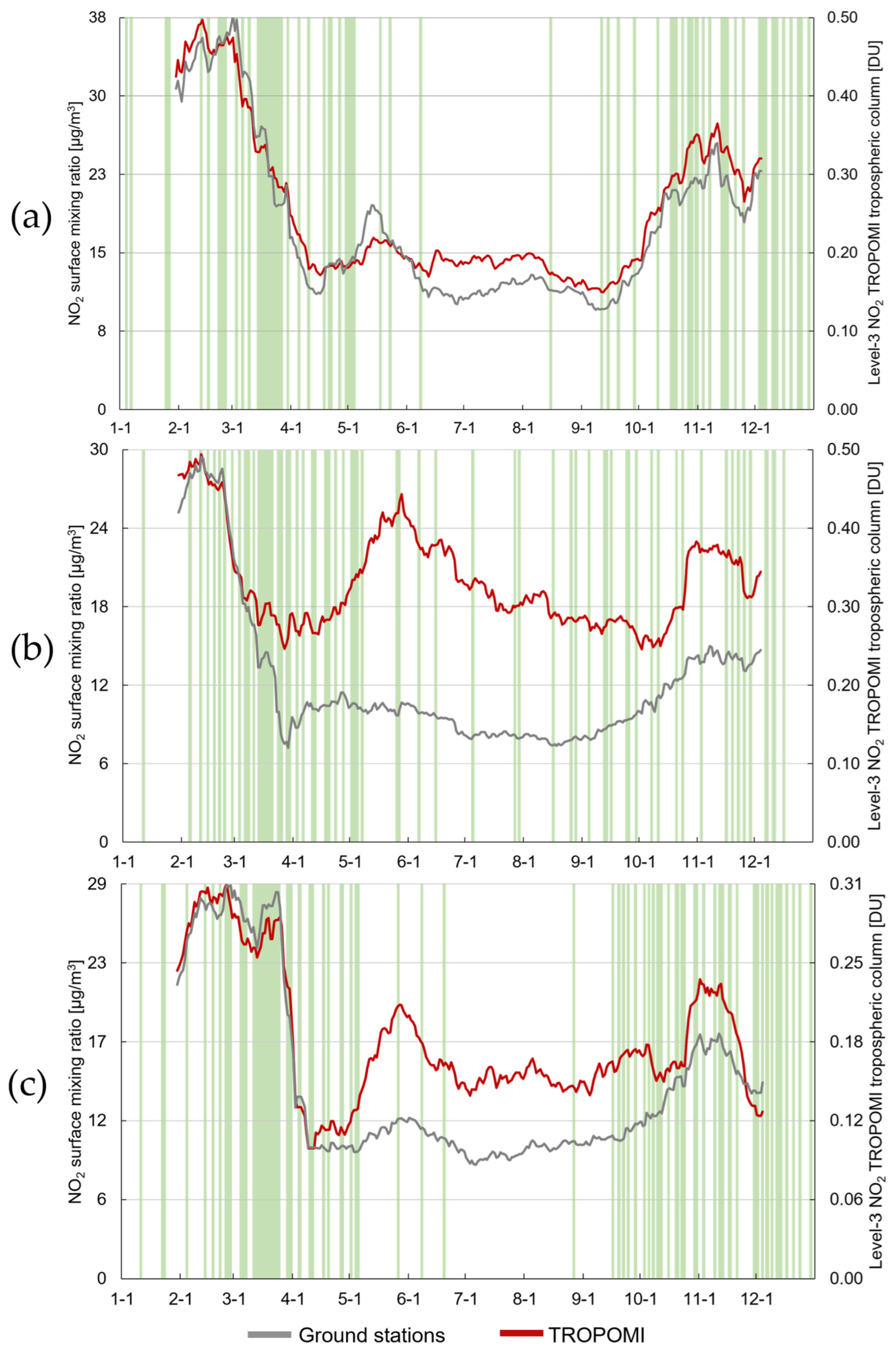
The temporal evolution of in situ and satellite NO2 concentration data were compared first. The analysis was limited to those cases where both types of observations could be retrieved simultaneously. Tropospheric column density data from TROPOMI displayed a more evident seasonal pattern in all three cities, with higher mean values in autumn and winter. In Madrid, both datasets aligned closely. However, measurements from air quality monitoring stations showed significant spikes in Barcelona and Valencia during warmer months, which were not clearly observed through satellite remote sensing (Figure 2).

Figure 2.
The 30-day moving average of NO2 concentration measured by the air quality monitoring stations networks and by TROPOMI in (a) Madrid, (b) Barcelona, and (c) Valencia in 2022. Green background highlights the days for which no valid satellite observations were available due to quality constraints.
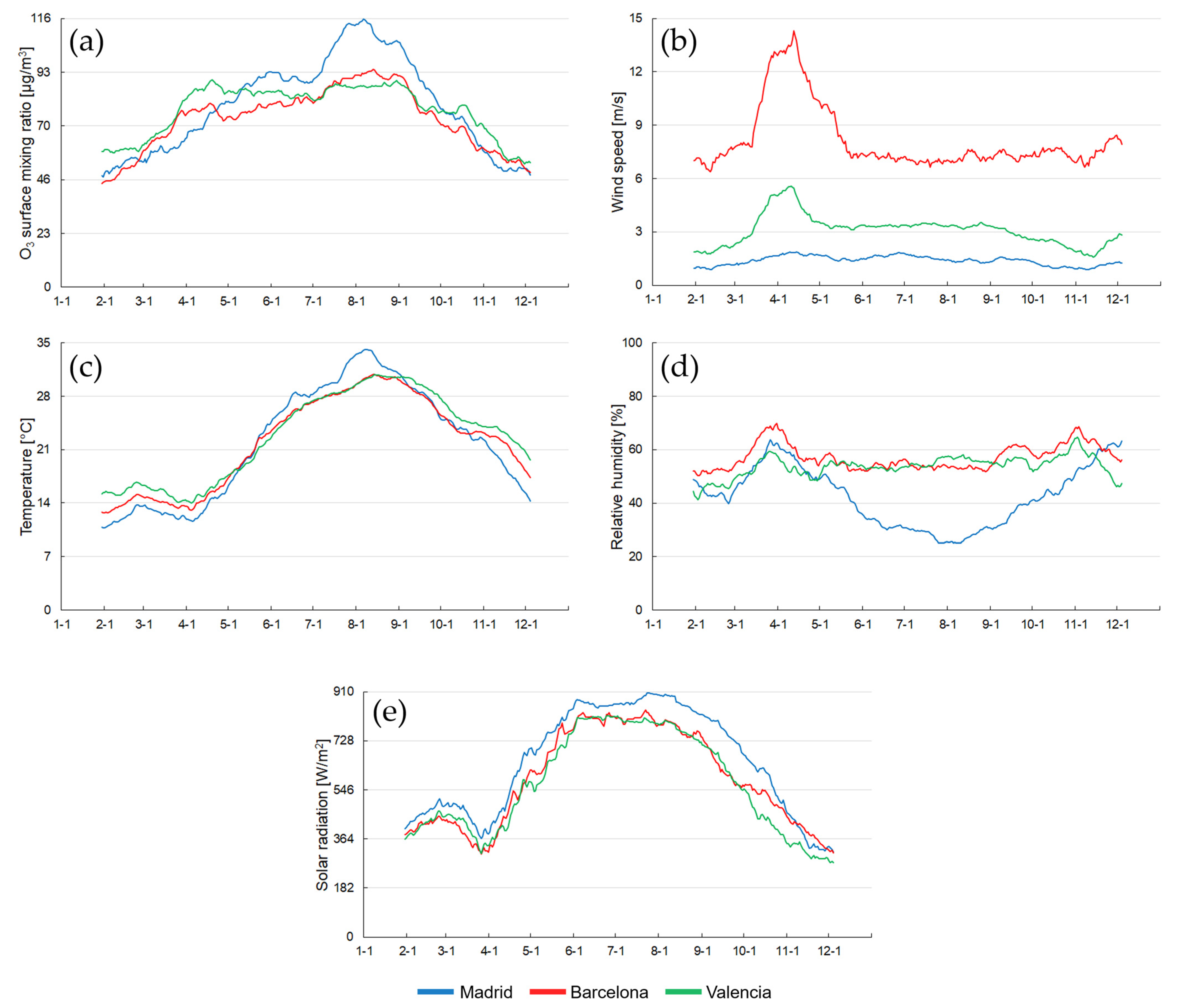
The temporal evolution of the rest of the variables is depicted in Figure 3.

Figure 3.
The 30-day moving average of (a) O3 surface concentration, (b) wind speed, (c) temperature, (d) relative humidity, and (e) solar radiation in (blue) Madrid, (red) Barcelona, and (green) Valencia in 2022.
O3 surface concentration developed similarly in the three cities. It decreased during colder months and spiked in summer, although this enhancement was more significant in Madrid (Figure 3a).
Wind speed (Figure 3b) and relative humidity (Figure 3d) showed similar patterns in the coastal cities. Wind speed was more intense during spring, and relative humidity maintained a relatively constant distribution, with slight increases in spring and autumn. In contrast, opposite trends were observed in Madrid. Wind speed remained more uniform throughout the year, while relative humidity experienced a significant decrease during the summer.
Temperature (Figure 3c) and solar radiation (Figure 3e) followed similar trends in all three cities, increasing from early spring until August, when the seasonal decline began.
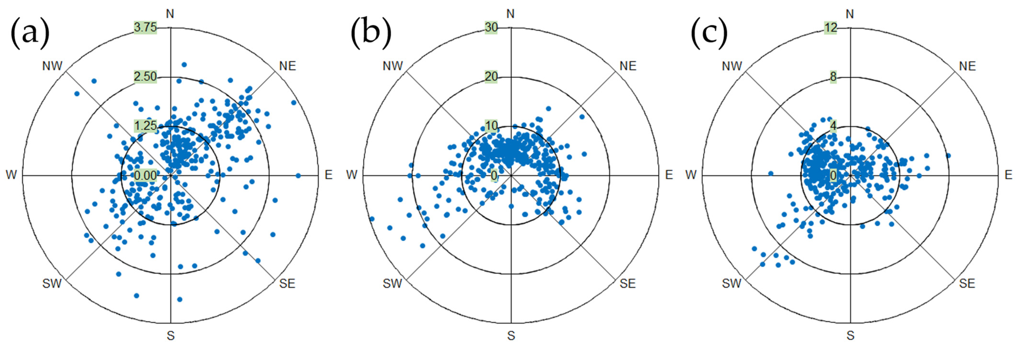
Wind distribution is represented separately in Figure 4. In Madrid, 54.5% of wind observations (Figure 4a) were recorded in the N and NE directions, with an average speed of 1.44 m/s. In Barcelona (Figure 4b), 61.1% of observations were recorded between NW and NE directions, with an average speed of 8.63 m/s. In Valencia (Figure 4c), 54.2% of observations were recorded between the W and NW directions, with an average speed of 2.73 m/s.

Figure 4.
Distribution of wind speed and direction in 2022 in (a) Madrid, (b) Barcelona, and (c) Valencia, where N stands for north (337.5–22.5°), NE for northeast (22.5–67.5°), E for east (67.5–112.5°), SE for southeast (112.5–157.5°), S for south (157.5–202.5°), SW for southwest (202.5–247.5°), W for west (247.5–292.5°), and NW for northwest (292.5–337.5°). Each dot represents average wind speed and direction in a day between Sentinel-5P overpass times. The distance to the center corresponds to the speed magnitude, and the angle with respect to the N represents the direction.
3.3. Correlation Between NO2 and Meteorological Variables
Table 2 shows the correlation coefficient matrix. The first column displays the relationship between both NO2 datasets, which align with the graphics in Figure 2.
Table 2.
Linear correlation coefficients (r) between NO2 data from air quality monitoring stations and TROPOMI and between the studied meteorological variables in each city. Values marked with an asterisk (*) are not statistically significant at p < 0.05.
In all three cities, O3 had the strongest correlation with both NO2 datasets. Wind speed coefficients were close to those of O3, and very similar within each location. Temperature results showed greater discrepancies between ground and satellite data in the coastal cities (r = −0.10 vs. r = −0.46 in Barcelona; r = −0.17 vs. r = −0.48 in Valencia). This was also the case for solar radiation (r = −0.17 vs. r = −0.41 in Barcelona; r = −0.18 vs. r = −0.40 in Valencia). Relative humidity was the only variable that showed positive correlation coefficients, which did not exceed r = 0.3 in any case.
All correlation coefficients presented in Table 2 were tested for statistical significance using Pearson’s correlation test. In all three cities, most correlations between NO2 and meteorological variables—including O3, wind speed, temperature (except for AQ stations data in Barcelona), and solar radiation—were statistically significant (p < 0.05). Only correlations involving relative humidity showed non-significant values (p > 0.05), indicating that the weak relationships observed may not result from consistent patterns.
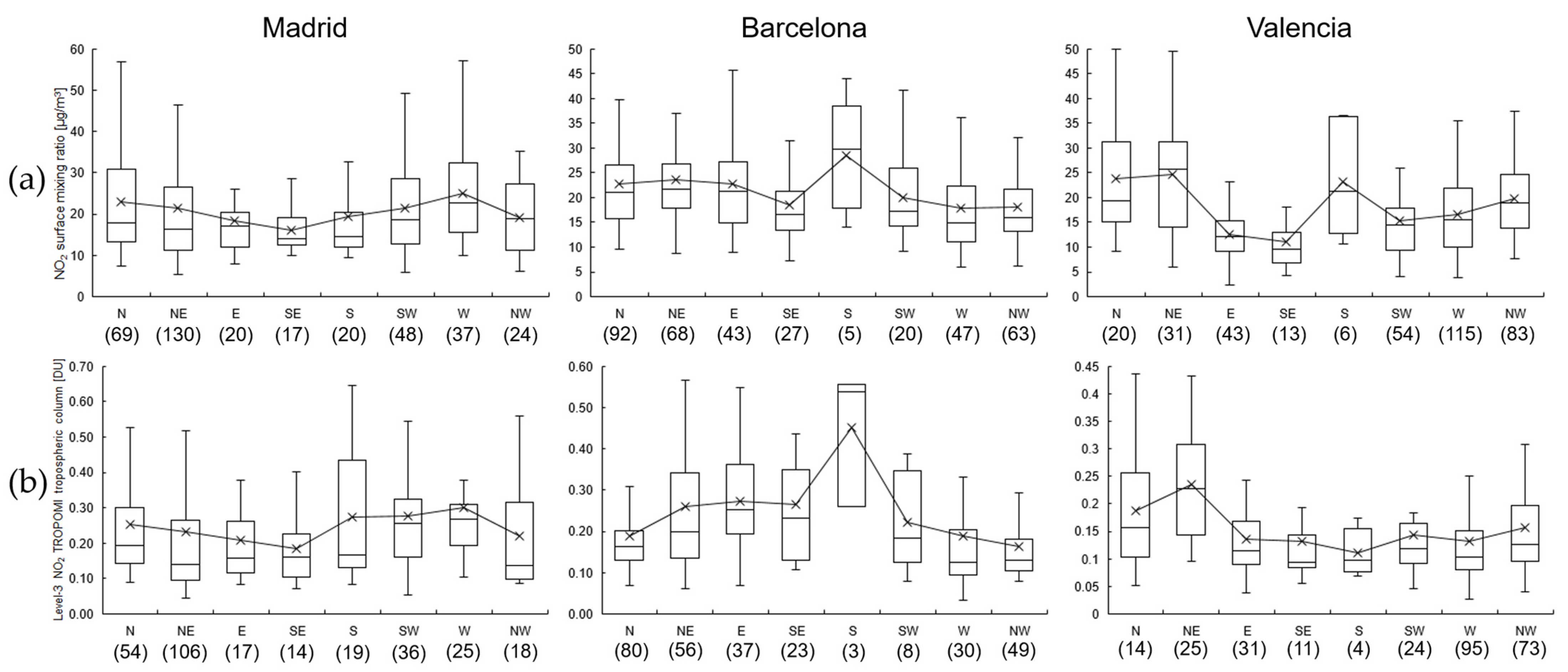
Figure 5 displays the distribution of NO2 concentration according to wind direction.

Figure 5.
Boxplot of NO2 concentration data measured by (a) air quality monitoring stations and (b) TROPOMI depending on wind direction in each city in 2022. The number of cases for each direction is indicated in parentheses.
The results were similar for both air quality monitoring stations (Figure 5a) and TROPOMI (Figure 5b) data. In Madrid, the lowest and highest NO2 concentrations were observed for the SE (16 µg/m3 and 0.184 DU) and W (25.1 µg/m3 and 0.302 DU) directions, respectively, although with very slight differences. In Barcelona, these cases were observed for the NW (18.2 µg/m3 and 0.162 DU) and S (28.4 µg/m3 and 0.451 DU) directions, although S was the least frequent direction. Valencia showed more discrepancies than the other cities, although the highest concentrations were detected for the NE (24.6 µg/m3 and 0.235 DU).
A side-by-side comparison between Figures S2 and S3, Figures S4–S7 provides a more in-depth analysis of the influence of the wind on the spatial distribution of NO2 concentration. In periods of higher speeds and more persistent directions, pollution hotspots tended to shift accordingly. This is particularly noticeable in Barcelona and Valencia, where wind speeds were consistently higher than in Madrid.
3.4. Study Variables Under Extreme NO2 Conditions
Table 3 shows the average conditions in the top 10% and bottom 10% cases of NO2 pollution.
Table 3.
Average value of all study variables in the top 10% and bottom 10% (in parentheses) NO2 concentration scenarios observed by air quality monitoring stations and TROPOMI in each city in 2022.
In all three cities, top and bottom NO2 and O3 concentrations were inversely related. The same pattern was observed for wind speed, temperature, and solar radiation, but not for relative humidity.
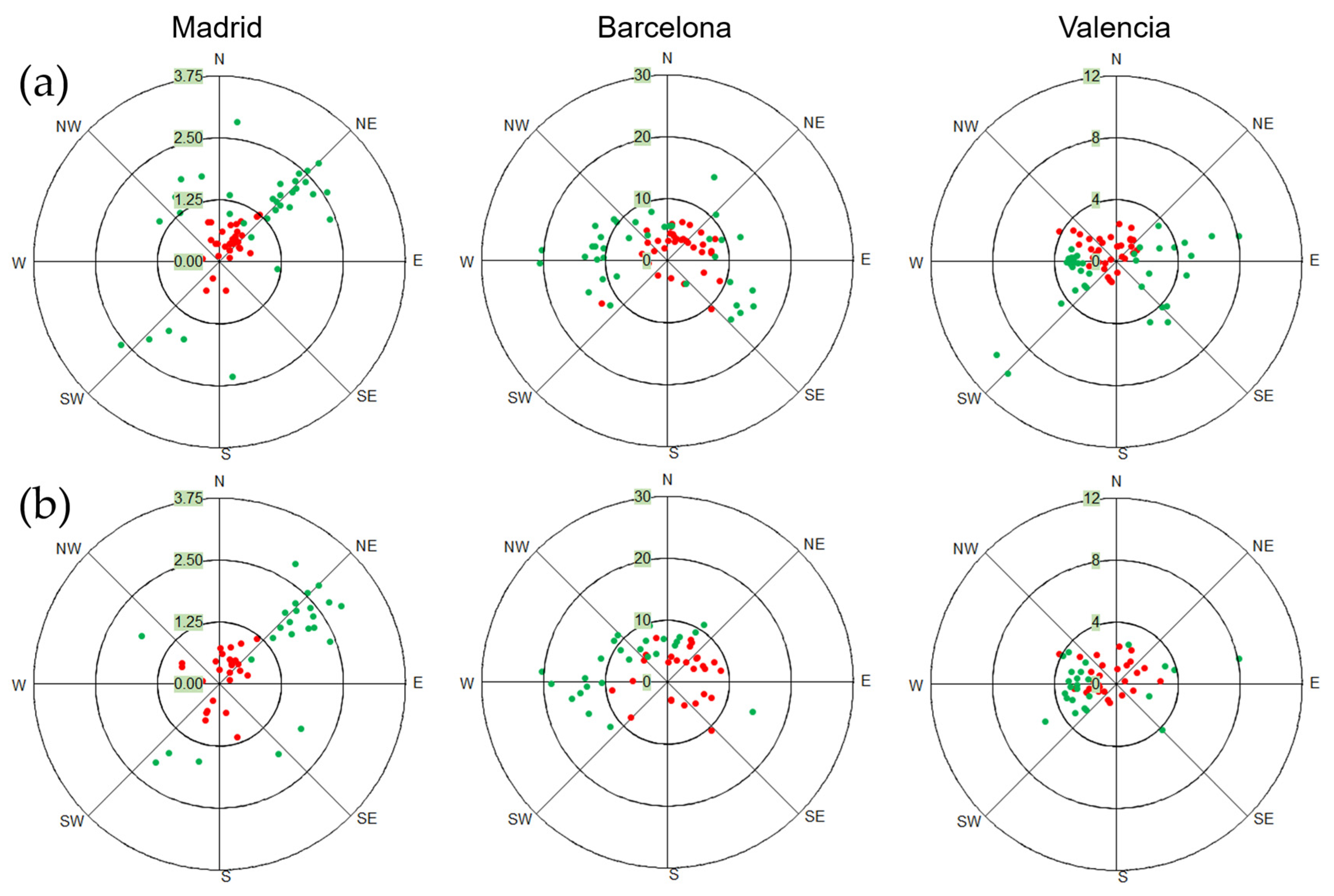
Extreme NO2 data according to wind records are shown in Figure 6. In Madrid, most results accumulated in the NE direction, with wind speed being a determining factor.

Figure 6.
Wind speed and wind direction records in the top 10% (red) and bottom 10% (green) NO2 concentration scenarios observed (a) by air quality monitoring stations and (b) by TROPOMI in each city in 2022.
Barcelona presented a more scattered distribution: air quality stations (Figure 6a) observed top NO2 episodes accumulating between the NW and E, while bottom cases depended on wind speed. TROPOMI (Figure 6b) detected most top NO2 episodes when the wind blew towards the sea, and bottom cases occurred for opposite directions. In Valencia, top NO2 episodes frequently gathered between the W and NE, while most bottom cases took place towards the W direction.
3.5. Principal Component Analysis
PCAs were conducted in all cases to further analyze patterns between NO2 concentration and all study variables. Table 4 shows the main results, with the original variables clustered in each principal component.
Table 4.
Main results of the PCA application for the study variables at Madrid, Barcelona, and Valencia for each NO2 dataset. Values in bold indicate the variables grouped in each principal component.
There was a consistent pattern in all performed PCAs. O3 concentration, temperature, and solar radiation were always placed in the same group. Wind speed was also closely related to NO2 concentration, in agreement with the correlation matrix in Table 2. Relative humidity was not associated with other variables.
In summary, the results show that NO2 concentrations were highest in Madrid, followed by Valencia and Barcelona, both in satellite-based and in situ datasets. Temporal trends and 30-day moving averages showed similar seasonal patterns across data sources, with higher values during colder months. Correlation analysis indicated a consistent negative association between NO2 and O3, temperature, wind speed, and solar radiation in all three cities. The strongest linear correlation between satellite and surface NO2 data was observed in Madrid (r = 0.86), followed by Valencia (r = 0.68) and Barcelona (r = 0.65). The PCAs grouped related meteorological and pollution variables into distinct components, which varied by city.
4. Discussion
The results of this research are based on the officially available meteorological and air quality information in each study region. The most accurate approach to this study was to have simultaneous measurements of NO2 and meteorological variables at the same locations. However, air quality and meteorological devices are not usually installed at the same points (Figure S2); thus, regional average values were obtained.
It should be noted that this study establishes a comparison between NO2 observations of different natures. Ground stations measure surface-level mixing ratio, while satellites provide atmospheric column density data. Due to the origin and nature of NO2, which has a short lifetime and mostly accumulates in the troposphere [18,53,54], both data groups show strong correlations in urban environments.
The linear correlation coefficients between in situ stations and TROPOMI NO2 data were stronger in Madrid (r = 0.86) than in Barcelona (r = 0.65) and Valencia (r = 0.68). The temporal evolution of NO2 pollution observed by satellite in all three cities followed a similar seasonal pattern. However, ground stations in Valencia and Barcelona detected an increase during spring that could not be entirely captured by TROPOMI. This discrepancy may partially be due not only to the influence of meteorological conditions on the NO2 vertical profile but also to data availability (Table S1). Madrid has a larger in situ data series because its monitoring infrastructure is more extensive and has been active for a long time. On the other hand, Sentinel-5P always provides at least one daily observation (Table 1), which sometimes does not meet the pixel quality criteria. The proximity to emission sources must also be considered. Previous studies have found that TROPOMI encounters limitations in detecting spatial gradients of NO2 concentration at smaller scales, particularly when compared to ground stations influenced by heavily trafficked roads or industrial plants [10,22]. These discrepancies could be more evident in cities with more limited air quality networks, such as Barcelona and Valencia (8 and 10 stations, respectively, compared to 24 in Madrid).
The geographical location and topography of each settlement can definitely play an important role as well. Madrid is placed in a mountain basin that limits movements between air layers during thermal inversion processes [55]. These conditions facilitate the retrieval of high quality pixel satellite images, resulting in a wider availability of TROPOMI data. Barcelona and Valencia are set at sea level on the Mediterranean coast, and experience more heterogeneous climatic conditions due to their proximity to the coastline. Wind speed data are the most evident case (Figure 4), as stronger winds induce air transport (Figures S2–S7) and mixing phenomena that hinder the immediate identification of surface-level pollution hotspots the emission sources. This may be the main reason why in Madrid, where the average wind speed is lower, in situ and satellite NO2 datasets align more closely compared to the coastal cities. At the same time, this influence on the dispersion of air pollutants is reflected in the correlation coefficients in Table 2. In fact, wind speed was the only meteorological variable that yielded similar results across all cases.
The correlation coefficients of temperature and solar radiation with NO2 data were equivalent, as they are highly related variables. Once emitted, the mean NO2 lifetime is longer in winter than in summer. This difference is attributed to higher exposure to UV radiation during summer months, which triggers photolysis processes and chemical conversion into other substances [56]. The photolysis rate depends on the presence of aerosols, solar zenith angle, cloud cover, and temperature itself [57,58]. This seasonality is emphasized by the use of domestic heating during cold periods, which adds to the usual road transport activities [11,59].
This is consistent with O3 concentration results, which presented the strongest negative correlation with both NO2 datasets. As a photochemical pollutant, tropospheric O3 is formed secondarily from reactions involving high solar radiation and temperature as well as other precursor gases, primarily NOx and volatile organic compounds (VOCs). Thus, tropospheric O3 levels rise in spring and summer, as opposed to NO2 (Figure 3a) [60,61]. Furthermore, O3 can undergo titration processes by NO, leading to an increase in NO2 concentration.
The correlation between temperature and solar radiation with both NO2 datasets was consistent in Madrid. In Barcelona and Valencia, a stronger correlation was only observed with TROPOMI observations. Notably, the highest average solar radiations were recorded in Madrid (Table 1), with the bottom 10% of NO2 pollution cases taking place under 831 W/m2 (Table 3).
Relative humidity showed no significant relationships with NO2 pollution levels. In Madrid, a correlation coefficient of r = 0.30 was observed with air quality stations data (Table 2). Although humidity contributes to atmospheric transport processes through the formation of aerosol particles or wet deposition of pollutants, this value might result from a combination of the seasonal nature of emissions in Madrid and the prevalence of drier weather in the city during summer.
PCA results were coherent with these findings. Two main groups, or principal components, were constantly differentiated: one included O3 levels, temperature, and solar radiation; and the other, wind speed (Table 4). NO2 concentration always fell into one of these two clusters, meaning that to understand its variability and make accurate estimations, their information will be the most important.
Wind direction also plays a key role, but requires a separate analysis for each case. It determines how air masses are distributed away from or towards the sampling points and can significantly influence atmospheric composition, as shown in Figures S2–S7. Figure 5 depicts a similar distribution of NO2 levels across wind directions for both data groups. In Madrid, the wind regime (Figure 4a) is shaped by its geographical location, set at the base of one of the main mountain chains of the Iberian Peninsula, the Central System, which divide its core from NE to SW. This is the cause of such persistent directions, leading to pollution being more dependent on wind speed (Figure 6). In Barcelona and particularly Valencia, where winds are consistently stronger, these patterns are influenced by their proximity to the coastline. In Barcelona, scenarios of higher pollution were more frequently observed between the NW and E, albeit with a widely scattered distribution. In Valencia, the worst air quality cases gathered between the NW and NE directions, whereas cleaner air events were associated with W winds. This means that information on wind direction is essential for characterizing changes in air quality in these locations but not so much in Madrid.
These findings are consistent with comparable research using air quality monitoring stations [26] and satellite imagery [27], which emphasize the importance of conducting individual analyses for each study region. In urban settings specifically, atmospheric composition is shaped by a multitude of interconnected drivers. In the cases referred to here, the most defining variables differ between inland and coastal cities. However, this information is not often considered for activating action protocols under high pollution episodes, and can definitely be used for making surface-level estimations.
This methodology could potentially be adapted to smaller municipalities by incorporating proxy variables such as land use, traffic density, and emission sources. Future satellite missions like Sentinel-4 may also enhance data availability for urban areas with more complex topography or limited monitoring infrastructure.
Certain methodological considerations should be acknowledged. The spatial resolution of Sentinel-5P, though improved, is still insufficient to capture fine-scale variability in NO2 concentrations at the street level, particularly in dense urban areas. Satellite data availability is also subject to quality constraints due to factors such as cloud cover or low-quality retrievals. Additionally, the statistical approach followed here focused on identifying linear associations between variables. While this method is appropriate for exploring dominant patterns, non-linear interactions may require alternative analytical frameworks and could be addressed in future research.
5. Conclusions
Current Spanish action protocols for high-NO2 pollution episodes do not consider meteorological scenarios for the assessment of severity and duration. Understanding the atmospheric dynamics of NO2 in urban environments is key to policymaking and compliance with air quality guidelines. This study explored the relationship between O3 levels, five meteorological variables (wind speed, wind direction, temperature, relative humidity, and solar radiation), and the average NO2 concentration from air quality stations and the TROPOMI sensor in the cities of Madrid, Barcelona, and Valencia during 2022. These locations were chosen due to significant NO2 exposure concerns, which have not been previously addressed by comparing in situ and satellite data. The outcome helps identify the similarities and discrepancies between both datasets for making surface-level estimations.
Regional daily mean values were obtained between Sentinel-5P overpass times, which consistently occur between 12 p.m. and 4 p.m. TROPOMI data were obtained at the geographical position of the air quality monitoring stations. This methodology aligns with previous similar research [53,62].
In Madrid, NO2 satellite measurements followed a similar trend to in situ data, yielding a high linear correlation coefficient (r = 0.86). In Barcelona (r = 0.65) and Valencia (r = 0.68), most discrepancies were found during warmer months. A preliminary statistical analysis revealed that Madrid’s meteorological profile was also more stable than that of coastal cities, especially regarding wind speed and direction, which are heavily influenced by geographical location and orographic configuration. Their effect on the NO2 formation, removal, mixing, or transport affects the relationship between atmospheric column and surface concentrations. As average wind speed increased, the correlation between NO2 datasets decreased. The emissions profile of each location (which depends on the activity and time of year) and data availability must also be considered. Madrid has a network of 24 air quality stations for NO2, compared to 8 in Barcelona and 10 in Valencia. Their proximity to emission sources can limit the comparison, since small spatial gradients are hardly noticeable via satellite. In addition, the availability of Sentinel-5P images varied across locations due to pixel quality criteria.
A correlation analysis showed that increased O3 pollution and wind speed were linked to lower NO2 concentrations in all three cities for both datasets. This is due to O3 and NO2 being involved in opposite formation processes, and wind speed promoting their dispersion. Temperature and solar radiation also presented an inverse relationship, as they trigger NO2 photolysis (and hence O3 formation). However, the results using in situ and satellite data were only comparable in Madrid. The distribution of NO2 concentration based on wind direction showed an overall good agreement, although air quality in Madrid was more dependent on wind speed. Relative humidity did not show significant correlations in any case. The PCAs identified and confirmed these connections, with slight differences across cities and datasets. NO2 was consistently associated with two clusters: one formed by O3 concentration, temperature and solar radiation, and the other by wind speed.
These variations emphasize the need to study each location in order to evaluate the impact of meteorology on atmospheric pollution. According to the above results, the most influential study variables in air quality are O3, wind speed, temperature, and solar radiation in Madrid; and O3, wind speed, and wind direction in Barcelona and Valencia. Due to their consistency with in situ and satellite NO2 datasets, this information is of great value to make accurate surface-level estimations, which will be the target of further research.
Future efforts should also focus on studying land cover, land use, and other existing features to better describe the role of anthropogenic factors in the regional distribution of NO2. Surface-level data from other pollutants (e.g., particulate matter, SO2, CO), could be of interest to gain insight into atmospheric conversion and removal processes. Eventually, air quality studies conducted via remote sensing will be particularly valuable in regions lacking monitoring infrastructure and for assessing the effectiveness of impact and mitigation policies from a regional perspective. This is especially relevant in Spain’s current context, where legislation is being adapted to the European 2030 climate and energy framework.
Supplementary Materials
The following supporting information can be downloaded at: https://www.mdpi.com/article/10.3390/nitrogen6020032/s1, Figure S1: Geographical location of air quality monitoring stations (red circles) and meteorological stations (blue triangles) in the cities of (a) Madrid, (b) Barcelona, and (c) Valencia. Numbers correspond to those displayed in Table S1. Figure S2: Monthly maps of mean tropospheric TROPOMI NO2 column (DU) over Madrid and its surroundings in (a) January, (b) February, (c) March, (d) April, (e) May, (f) June, (g) July, (h) August, (i) September, (j) October, (k) November, and (l) December of 2022. Black lines represent the city limits. Figure S3: Monthly distribution of wind distribution in Madrid in 2022: January (a), February (b), March (c), April (d), May (e), June (f), July (g), August (h), September (i), October (j), November (k), and December (l). Blue dots represent average wind speed and direction in a day between Sentinel-5P overpass times. Figure S4: Monthly maps of mean tropospheric TROPOMI NO2 column (DU) over Barcelona and its surroundings in (a) January, (b) February, (c) March, (d) April, (e) May, (f) June, (g) July, (h) August, (i) September, (j) October, (k) November, and (l) December of 2022. Black lines represent the city limits. White lines represent the coastline. Figure S5: Monthly distribution of wind distribution in Barcelona in 2022: January (a), February (b), March (c), April (d), May (e), June (f), July (g), August (h), September (i), October (j), November (k), and December (l). Blue dots represent average wind speed and direction in a day between Sentinel-5P overpass times. Figure S6: Monthly maps of mean tropospheric TROPOMI NO2 column (DU) over Valencia and its surroundings in (a) January, (b) February, (c) March, (d) April, (e) May, (f) June, (g) July, (h) August, (i) September, (j) October, (k) November, and (l) December of 2022. Black lines represent the city limits. White lines represent the coastline. Figure S7: Monthly distribution of wind distribution in Valencia in 2022: January (a), February (b), March (c), April (d), May (e), June (f), July (g), August (h), September (i), October (j), November (k), and December (l). Blue dots represent average wind speed and direction in a day between Sentinel-5P overpass times. Table S1: Air quality monitoring stations, meteorological stations, and data availability in each city under study. Station numbers correspond to those displayed in Figure S1.
Author Contributions
Conceptualization, S.M., S.Á. and C.M.; methodology, C.M., J.C.M.P. and A.J.G.; software, S.Á., C.M. and A.J.G.; validation, S.M. and J.C.M.P.; formal analysis, C.M., S.M. and S.Á.; investigation, C.M., J.C.M.P. and A.J.G.; resources, S.M. and S.Á.; data curation, C.M., S.M. and S.Á.; writing—original draft preparation, C.M. and S.M.; writing—review and editing, S.Á., J.C.M.P., and A.J.G.; visualization, C.M., S.M. and S.Á.; supervision, J.C.M.P. and A.J.G.; project administration, S.M. and S.Á.; funding acquisition, S.Á. All authors have read and agreed to the published version of the manuscript.
Funding
This research was funded by (i) Project TED2021-130457A-I00, funded by MCIN/AEI/10.13039/501100011033 and European Union “NextGenerationEU”/PRTR” (Grant ID: Sergio Alvarez) and (ii) UIDB/00511/2020 (DOI: 10.54499/UIDB/00511/2020), UIDP/00511/2020 (DOI: 10.54499/UIDP/00511/2020, LEPABE), and LA/P/0045/2020 (DOI: 10.54499/LA/P/0045/2020, ALiCE), funded by national funds through FCT/MCTES (PIDDAC) (Grant ID: Jose CM Pires).
Data Availability Statement
The original contributions presented in this study are included in the article/Supplementary Materials. Further inquiries can be directed to the corresponding author(s).
Conflicts of Interest
The authors declare no conflicts of interest. The funders had no role in the design of the study; in the collection, analyses, or interpretation of data; in the writing of the manuscript; or in the decision to publish the results.
References
- Martin, R.V.; Jacob, D.J.; Chance, K.; Kurosu, T.P.; Palmer, P.I.; Evans, M.J. Global Inventory of Nitrogen Oxide Emissions Constrained by Space-Based Observations of NO2 Columns. J. Geophys. Res. Atmos. 2003, 108, 4537. [Google Scholar] [CrossRef]
- Oppenheimer, C.; Kyle, P.R.; Tsanev, V.I.; McGonigle, A.J.S.; Mather, T.A.; Sweeney, D. Mt. Erebus, the Largest Point Source of NO2 in Antarctica. Atmos. Environ. 2005, 39, 6000–6006. [Google Scholar] [CrossRef]
- McDuffie, E.E.; Smith, S.J.; O’Rourke, P.; Tibrewal, K.; Venkataraman, C.; Marais, E.A.; Zheng, B.; Crippa, M.; Brauer, M.; Martin, R.V. A Global Anthropogenic Emission Inventory of Atmospheric Pollutants from Sector- And Fuel-Specific Sources (1970–2017): An Application of the Community Emissions Data System (CEDS). Earth Syst. Sci. Data 2020, 12, 3413–3442. [Google Scholar] [CrossRef]
- Shaw, S.; Van Heyst, B. An Evaluation of Risk Ratios on Physical and Mental Health Correlations Due to Increases in Ambient Nitrogen Oxide (NOx) Concentrations. Atmosphere 2022, 13, 967. [Google Scholar] [CrossRef]
- Jonson, J.E.; Borken-Kleefeld, J.; Simpson, D.; Nyíri, A.; Posch, M.; Heyes, C. Impact of Excess NOx Emissions from Diesel Cars on Air Quality, Public Health and Eutrophication in Europe. Environ. Res. Lett. 2017, 12, 094017. [Google Scholar] [CrossRef]
- Kwon, H.; Cho, N. Corrosion Behaviors of Outdoor Bronze Sculptures in an Urban–Industrial Environment: Corrosion Experiment on Artificial Sulfide Patina. Metals 2023, 13, 1101. [Google Scholar] [CrossRef]
- United Nations (UN). World Urbanization Prospects 2018. Available online: https://population.un.org/wup/assets/WUP2018-Highlights.pdf (accessed on 12 February 2024).
- World Health Organization (WHO). WHO Global Air Quality Guidelines: Particulate Matter (PM2.5 and PM10), Ozone, Nitrogen Dioxide, Sulfur Dioxide and Carbon Monoxide. 2021. Available online: https://www.who.int/publications/i/item/9789240034228 (accessed on 12 February 2024).
- Khomenko, S.; Cirach, M.; Pereira-Barboza, E.; Mueller, N.; Barrera-Gómez, J.; Rojas-Rueda, D.; de Hoogh, K.; Hoek, G.; Nieuwenhuijsen, M. Premature Mortality Due to Air Pollution in European Cities: A Health Impact Assessment. Lancet Planet. Heal. 2021, 5, e121–e134. [Google Scholar] [CrossRef]
- Goldberg, D.L.; Anenberg, S.C.; Kerr, G.H.; Mohegh, A.; Lu, Z.; Streets, D.G. TROPOMI NO2 in the United States: A Detailed Look at the Annual Averages, Weekly Cycles, Effects of Temperature, and Correlation With Surface NO2 Concentrations. Earth’s Futur. 2021, 9, e2020EF001665. [Google Scholar] [CrossRef] [PubMed]
- Morillas, C.; Alvarez, S.; Pires, J.C.M.; Garcia, A.J.; Martinez, S. Impact of the Implementation of Madrid’s Low Emission Zone on NO2 Concentration Using Sentinel-5P/TROPOMI Data. Atmos. Environ. 2024, 320, 120326. [Google Scholar] [CrossRef]
- Petetin, H.; Guevara, M.; Compernolle, S.; Bowdalo, D.; Bretonnière, P.A.; Enciso, S.; Jorba, O.; Lopez, F.; Soret, A.; García-Pando, C.P. Potential of TROPOMI for Understanding Spatio-Temporal Variations in Surface NO2 and Their Dependencies upon Land Use over the Iberian Peninsula. Atmos. Chem. Phys. 2023, 23, 3905–3935. [Google Scholar] [CrossRef]
- Rudke, A.P.; Martins, J.A.; Hallak, R.; Martins, L.D.; de Almeida, D.S.; Beal, A.; Freitas, E.D.; Andrade, M.F.; Koutrakis, P.; Albuquerque, T.T.A. Evaluating TROPOMI and MODIS Performance to Capture the Dynamic of Air Pollution in São Paulo State: A Case Study during the COVID-19 Outbreak. Remote Sens. Environ. 2023, 289, 113514. [Google Scholar] [CrossRef]
- Veefkind, J.P.; Aben, I.; McMullan, K.; Förster, H.; de Vries, J.; Otter, G.; Claas, J.; Eskes, H.J.; de Haan, J.F.; Kleipool, Q.; et al. TROPOMI on the ESA Sentinel-5 Precursor: A GMES Mission for Global Observations of the Atmospheric Composition for Climate, Air Quality and Ozone Layer Applications. Remote Sens. Environ. 2012, 120, 70–83. [Google Scholar] [CrossRef]
- Eskes, H.; Van Geffen, J.; Boersma, F.; Eichmann, K.-U.; Apituley, A.; Pedergnana, M.; Sneep, M.; Veefkind, J.P.; Loyola, D. Sentinel-5 Precursor/TROPOMI Level 2 Product User Manual Nitrogendioxide Document Number: S5P-KNMI-L2-0021-MA. 2022. Available online: https://sentiwiki.copernicus.eu/__attachments/1673595/S5P-KNMI-L2-0021-MA%20-%20Sentinel-5P%20Level%202%20Product%20User%20Manual%20Nitrogendioxide%202024%20-%204.4.0.pdf?inst-v=4318c067-be91-4544-be2e-16af66246c9f (accessed on 12 February 2024).
- Eskes, H.J.; Eichmann, K.-U. S5P Mission Performance Centre Nitrogen Dioxide Readme L2; Royal Netherlands Meteorological Institute: De Bilt, The Netherlands, 2018; Available online: https://sentinel.esa.int/documents/247904/3541451/Sentinel-5P-Nitrogen-Dioxide-Level-2-Product-Readme-File.pdf (accessed on 12 February 2024).
- Griffin, D.; Zhao, X.; McLinden, C.A.; Boersma, F.; Bourassa, A.; Dammers, E.; Degenstein, D.; Eskes, H.; Fehr, L.; Fioletov, V.; et al. High-Resolution Mapping of Nitrogen Dioxide With TROPOMI: First Results and Validation Over the Canadian Oil Sands. Geophys. Res. Lett. 2019, 46, 1049–1060. [Google Scholar] [CrossRef]
- Lange, K.; Richter, A.; Burrows, J.P. Variability of Nitrogen Oxide Emission Fluxes and Lifetimes Estimated from Sentinel-5P TROPOMI Observations. Atmos. Chem. Phys. 2022, 22, 2745–2767. [Google Scholar] [CrossRef]
- Cersosimo, A.; Serio, C.; Masiello, G. TROPOMI NO2 Tropospheric Column Data: Regridding to 1 Km Grid-Resolution and Assessment of Their Consistency with In Situ Surface Observations. Remote Sens. 2020, 12, 2212. [Google Scholar] [CrossRef]
- Ialongo, I.; Virta, H.; Eskes, H.; Hovila, J.; Douros, J. Comparison of TROPOMI/Sentinel-5 Precursor NO2 Observations with Ground-Based Measurements in Helsinki. Atmos. Meas. Tech. 2020, 13, 205–218. [Google Scholar] [CrossRef]
- Jeong, U.; Hong, H. Assessment of Tropospheric Concentrations of NO2 from the TROPOMI/Sentinel-5 Precursor for the Estimation of Long-Term Exposure to Surface NO2 over South Korea. Remote Sens. 2021, 13, 1877. [Google Scholar] [CrossRef]
- Morillas, C.; Alvarez, S.; Serio, C.; Masiello, G.; Martinez, S. TROPOMI NO2 Sentinel-5P Data in the Community of Madrid: A Detailed Consistency Analysis with in Situ Surface Observations. Remote Sens. Appl. Soc. Environ. 2024, 33, 101083. [Google Scholar] [CrossRef]
- Giosanu, D.; Marian, M.C.; Zaharia, A. THE INFLUENCE OF METEOROLOGICAL AND TOPOGRAPHICAL PARAMETERS ON THE DISPERSION OF PM10 AND CO POLLUTANTS. Curr. Trends Nat. Sci. 2021, 10, 92–98. [Google Scholar] [CrossRef]
- Giovannini, L.; Ferrero, E.; Karl, T.; Rotach, M.W.; Staquet, C.; Castelli, S.T.; Zardi, D. Atmospheric Pollutant Dispersion over Complex Terrain: Challenges and Needs for Improving Air Quality Measurements and Modeling. Atmosphere 2020, 11, 646. [Google Scholar] [CrossRef]
- Zhang, X.; Qian, S.; Xu, J.; Cui, H.; Ma, R.; Gao, F. Relationship between Meteorological Factors and Diffusion of Atmospheric Pollutants. Chem. Eng. Trans. 2018, 71, 1417–1422. [Google Scholar] [CrossRef]
- Zhang, H.; Wang, Y.; Hu, J.; Ying, Q.; Hu, X.M. Relationships between Meteorological Parameters and Criteria Air Pollutants in Three Megacities in China. Environ. Res. 2015, 140, 242–254. [Google Scholar] [CrossRef] [PubMed]
- Rahman, M.M.; Shuo, W.; Zhao, W.; Xu, X.; Zhang, W.; Arshad, A. Investigating the Relationship between Air Pollutants and Meteorological Parameters Using Satellite Data over Bangladesh. Remote Sens. 2022, 14, 2757. [Google Scholar] [CrossRef]
- Adams, T.J.; Geddes, J.A.; Lind, E.S. New Insights Into the Role of Atmospheric Transport and Mixing on Column and Surface Concentrations of NO2 at a Coastal Urban Site. J. Geophys. Res. Atmos. 2023, 128, e2022JD038237. [Google Scholar] [CrossRef]
- Singh, A. Role of Atmospheric Boundary Layer (ABL) Height and Ventilation Coefficient on Urban Air Quality- A Study Based on Observations and NWP Model. J. Atmos. Sci. Res. 2019, 2, 11–16. [Google Scholar] [CrossRef]
- Su, T.; Li, Z.; Kahn, R. Relationships between the Planetary Boundary Layer Height and Surface Pollutants Derived from Lidar Observations over China: Regional Pattern and Influencing Factors. Atmos. Chem. Phys. 2018, 18, 15921–15935. [Google Scholar] [CrossRef]
- Karami, S.; Ghassabi, Z.; Khoddam, N.; Habibi, M. Investigating Meteorological Factors Influencing Pollutant Concentrations and Copernicus Atmosphere Monitoring Service (CAMS) Model Forecasts in the Tehran Metropolis. Atmosphere 2025, 16, 264. [Google Scholar] [CrossRef]
- Danek, T.; Weglinska, E.; Zareba, M. The Influence of Meteorological Factors and Terrain on Air Pollution Concentration and Migration: A Geostatistical Case Study from Krakow, Poland. Sci. Rep. 2022, 12, 11050. [Google Scholar] [CrossRef]
- Ahmad, N.; Lin, C.; Lau, A.K.H.; Kim, J.; Li, C.; Qin, K.; Zhao, C.; Lin, J.; Fung, J.C.H.; Li, Y. Effects of Meteorological Conditions on the Mixing Height of Nitrogen Dioxide in China Using New-Generation Geostationary Satellite Measurements and Machine Learning. Chemosphere 2024, 346, 140615. [Google Scholar] [CrossRef]
- Instituto Nacional de Estadística (INE). Cifras Oficiales de Población de Los Municipios Españoles En Aplicación de La Ley de Bases Del Régimen Local (Art. 17). Available online: https://www.ine.es/dynt3/inebase/index.htm?padre=525 (accessed on 13 March 2024).
- Ku, C.A.; Tsai, H.K. Evaluating the Influence of Urban Morphology on Urban Wind Environment Based on Computational Fluid Dynamics Simulation. ISPRS Int. J. Geo-Inf. 2020, 9, 399. [Google Scholar] [CrossRef]
- Melo, A.L.V.; Santos, J.M.; Reis, N.C.; Castro, I.P.; Goulart, E.V.; Xie, Z.T. Influence of Wind Direction and Source Location on Peak-to-Mean Concentration Ratios in Urban Environments. J. Wind Eng. Ind. Aerodyn. 2023, 232, 105264. [Google Scholar] [CrossRef]
- Muñoz Sabater, J. ERA5-Land Hourly Data from 1950 to Present. 2019. Available online: https://cds.climate.copernicus.eu/datasets/reanalysis-era5-land?tab=download (accessed on 12 February 2024).
- Cedeno Jimenez, J.R.; Brovelli, M.A. NO2 Concentration Estimation at Urban Ground Level by Integrating Sentinel 5P Data and ERA5 Using Machine Learning: The Milan (Italy) Case Study. Remote Sens. 2023, 15, 5400. [Google Scholar] [CrossRef]
- Government of Valencia Air Quality and Meteorological Data. Available online: https://mediambient.gva.es/es/web/calidad-ambiental/datos-on-line (accessed on 12 February 2024).
- Government of Catalonia List of Meteorological Stations of Catalonia. Available online: https://www.meteo.cat/observacions/llistat-xema (accessed on 12 February 2024).
- Government of Catalunya Air Quality Data. Available online: https://mediambient.gencat.cat/ca/05_ambits_dactuacio/atmosfera/qualitat_de_laire/vols-saber-que-respires/descarrega-de-dades/descarrega-dades-automatiques/ (accessed on 12 February 2024).
- City of Madrid Meteorological Data Since 2019. Available online: https://datos.madrid.es/sites/v/index.jsp?vgnextoid=fa8357cec5efa610VgnVCM1000001d4a900aRCRD&vgnextchannel=374512b9ace9f310VgnVCM100000171f5a0aRCRD (accessed on 12 February 2024).
- Ayuntamiento de Madrid Datos de Calidad Del Aire Desde 2001. Available online: https://datos.madrid.es/portal/site/egob/menuitem.c05c1f754a33a9fbe4b2e4b284f1a5a0/?vgnextoid=aecb88a7e2b73410VgnVCM2000000c205a0aRCRD&vgnextchannel=374512b9ace9f310VgnVCM100000171f5a0aRCRD (accessed on 17 April 2023).
- Caleta, L.; Gulde, S.T.; Kolm, M.G.; Smith, D.J.; Maurer, R.; Bazalgette Courrèges-Lacoste, G.; Sallusti, M.; Bagnasco, G. Sentinel 4: A Geostationary Imaging UVN Spectrometer for Air Quality Monitoring: Status of Design, Performance and Development. In Proceedings of the International Conference on Space Optics—ICSO 2014, Tenerife, Canary Islands, Spain, 7–10 October 2014; Volume 10563, pp. 1158–1166. [Google Scholar] [CrossRef]
- Irizar, J.; Melf, M.; Bartsch, P.; Koehler, J.; Weiss, S.; Greinacher, R.; Erdmann, M.; Kirschner, V.; Perez Albinana, A.; Martin, D. Sentinel-5/UVNS. In Proceedings of the International Conference on Space Optics-ICSO 2018, Chania, Greece, 9–12 October 2018; Volume 11180, pp. 41–58. [Google Scholar] [CrossRef]
- Van Geffen, J.H.G.M.; Eskes, H.J.; Boersma, K.F.; Maasakkers, J.D.; Veefkind, J.P. TROPOMI ATBD of the Total and Tropospheric NO2 Data Products. 2019. Available online: https://sentinel.esa.int/documents/247904/2476257/Sentinel-5P-TROPOMI-ATBD-NO2-data-products.pdf (accessed on 12 February 2024).
- European Space Agency Data Products-Sentinel-5P Mission. Available online: https://sentinels.copernicus.eu/web/sentinel/missions/sentinel-5p/data-products (accessed on 12 February 2024).
- Williams, J.E.; Folkert Boersma, K.; Le Sager, P.; Verstraeten, W.W. The High-Resolution Version of TM5-MP for Optimized Satellite Retrievals: Description and Validation. Geosci. Model Dev. 2017, 10, 721–750. [Google Scholar] [CrossRef]
- Earth Engine Data Catalog Sentinel-5P OFFL NO2: Offline Nitrogen Dioxide. Available online: https://developers.google.com/earth-engine/datasets/catalog/COPERNICUS_S5P_OFFL_L3_NO2#description (accessed on 17 April 2023).
- Pires, J.C.M.; Sousa, S.I.V.; Pereira, M.C.; Alvim-Ferraz, M.C.M.; Martins, F.G. Management of Air Quality Monitoring Using Principal Component and Cluster Analysis—Part II: CO, NO2 and O3. Atmos. Environ. 2008, 42, 1261–1274. [Google Scholar] [CrossRef]
- Infostat-Software Estadístico. Available online: https://www.infostat.com.ar/ (accessed on 25 April 2025).
- Cedeno Jimenez, J.R.; Pugliese Viloria, A.D.J.; Brovelli, M.A. Estimating Daily NO2 Ground Level Concentrations Using Sentinel-5P and Ground Sensor Meteorological Measurements. ISPRS Int. J. Geo-Inf. 2023, 12, 107. [Google Scholar] [CrossRef]
- Shah, V.J.; Jacob, D.; Li, K.; Silvern, R.; Zhai, S.; Liu, M.; Lin, J.; Zhang, Q. Effect of Changing NOx Lifetime on the Seasonality and Long-Term Trends of Satellite-Observed Tropospheric NO2 Columns over China. Atmos. Chem. Phys. 2020, 20, 1483–1495. [Google Scholar] [CrossRef]
- Laughner, J.L.; Cohen, R.C. Direct Observation of Changing NOx Lifetime in North American Cities. Science 2019, 366, 723–727. [Google Scholar] [CrossRef]
- Su, J.G.; Brauer, M.; Ainslie, B.; Steyn, D.; Larson, T.; Buzzelli, M. An Innovative Land Use Regression Model Incorporating Meteorology for Exposure Analysis. Sci. Total Environ. 2008, 390, 520–529. [Google Scholar] [CrossRef]
- Gorai, A.K.; Tuluri, F.; Tchounwou, P.B.; Ambinakudige, S. Influence of Local Meteorology and NO2 Conditions on Ground-Level Ozone Concentrations in the Eastern Part of Texas, USA. Air Qual. Atmos. Heal. 2015, 8, 81–96. [Google Scholar] [CrossRef]
- Eck, T.F.; Holben, B.N.; Kim, J.; Beyersdorf, A.J.; Choi, M.; Lee, S.; Koo, J.H.; Giles, D.M.; Schafer, J.S.; Sinyuk, A.; et al. Influence of Cloud, Fog, and High Relative Humidity during Pollution Transport Events in South Korea: Aerosol Properties and PM2.5 Variability. Atmos. Environ. 2020, 232, 117530. [Google Scholar] [CrossRef]
- Jayamurugan, R.; Kumaravel, B.; Palanivelraja, S.; Chockalingam, M.P. Influence of Temperature, Relative Humidity and Seasonal Variability on Ambient Air Quality in a Coastal Urban Area. Int. J. Atmos. Sci. 2013, 1, 264046. [Google Scholar] [CrossRef]
- Granier, C.; Darras, S.; van Der Gon, H.D.; Doubalova, J.; Elguindi, N.; Galle, B.; Gauss, M.; Guevara, M.; Jalkanen, J.-P.; Kuenen, J.; et al. The Copernicus Atmosphere Monitoring Service Global and Regional Emissions. Copernic. Atmos. Monit. Serv. 2019, 54. [Google Scholar] [CrossRef]
- Ravina, M.; Caramitti, G.; Panepinto, D.; Zanetti, M. Air Quality and Photochemical Reactions: Analysis of NOx and NO2 Concentrations in the Urban Area of Turin, Italy. Air Qual. Atmos. Heal. 2022, 15, 541–558. [Google Scholar] [CrossRef] [PubMed]
- Di Bernardino, A.; Mevi, G.; Iannarelli, A.M.; Falasca, S.; Cede, A.; Tiefengraber, M.; Casadio, S. Temporal Variation of NO2 and O3 in Rome (Italy) from Pandora and In Situ Measurements. Atmosphere 2023, 14, 594. [Google Scholar] [CrossRef]
- Lorente, A.; Boersma, K.F.; Eskes, H.J.; Veefkind, J.P.; van Geffen, J.H.G.M.; de Zeeuw, M.B.; Denier van der Gon, H.A.C.; Beirle, S.; Krol, M.C. Quantification of Nitrogen Oxides Emissions from Build-up of Pollution over Paris with TROPOMI. Sci. Rep. 2019, 9, 20033. [Google Scholar] [CrossRef]
Disclaimer/Publisher’s Note: The statements, opinions and data contained in all publications are solely those of the individual author(s) and contributor(s) and not of MDPI and/or the editor(s). MDPI and/or the editor(s) disclaim responsibility for any injury to people or property resulting from any ideas, methods, instructions or products referred to in the content. |
© 2025 by the authors. Licensee MDPI, Basel, Switzerland. This article is an open access article distributed under the terms and conditions of the Creative Commons Attribution (CC BY) license (https://creativecommons.org/licenses/by/4.0/).