Article

A Blind Few-Shot Learning for Multimodal-Biological Signals with Fractal Dimension Estimation

Division of Electronics and Electrical Engineering, Dongguk University, 30 Pildong-ro 1-gil, Jung-gu, Seoul 04620, Republic of Korea
*
Author to whom correspondence should be addressed.
Fractal Fract. 2025, 9(9), 585; https://doi.org/10.3390/fractalfract9090585
Submission received: 23 July 2025 / Revised: 16 August 2025 / Accepted: 1 September 2025 / Published: 3 September 2025

Abstract

Improving the decoding accuracy of biological signals has been a research focus for decades to advance health, automation, and robotic industries. However, challenges like inter-subject variability, data scarcity, and multifunctional variability cause low decoding accuracy, thus hindering the practical deployment of biological signal paradigms. This paper proposes a multifunctional biological signals network (Multi-BioSig-Net) that addresses the aforementioned issues by devising a novel blind few-shot learning (FSL) technique to quickly adapt to multiple target domains without needing a pre-trained model. Specifically, our proposed multimodal similarity extractor (MMSE) and self-multiple domain adaptation (SMDA) modules address data scarcity and inter-subject variability issues by exploiting and enhancing the similarity between multimodal samples and quickly adapting the target domains by adaptively adjusting the parameters’ weights and position, respectively. For multifunctional learning, we proposed inter-function discriminator (IFD) that discriminates the classes by extracting inter-class common features and then subtracts them from both classes to avoid false prediction of the proposed model due to overfitting on the common features. Furthermore, we proposed a holistic-local fusion (HLF) module that exploits contextual-detailed features to adapt the scale-varying features across multiple functions. In addition, fractal dimension estimation (FDE) was employed for the classification of left-hand motor imagery (LMI) and right-hand motor imagery (RMI), confirming that proposed method can effectively extract the discriminative features for this task. The effectiveness of our proposed algorithm was assessed quantitatively and statistically against competent state-of-the-art (SOTA) algorithms utilizing three public datasets, demonstrating that our proposed algorithm outperformed SOTA algorithms.

1. Introduction

Biological signals such as electrocardiogram (ECG) and electroencephalogram (EEG) are electrical signals produced by variations in chemical concentration (specifically in the heart and brain). These signals are used to capture the patterns of diseases and intentions [1,2,3]. These signals have been used in a wide range of applications, including health [2,4,5], motor imagery (MI) classification [6,7,8], and emotion recognition (ER) [9,10,11]. The abovementioned studies utilized biological signals to address the inter-subject variability and low signal-to-noise ratio (SNR) issues in apnea, MI, and ER classifications. However, their practical applications were confined due to the need for large data availability. Therefore, other studies leveraged deep learning and few-shot learning techniques to address the data scarcity, inter-subject variability, and low signal-to-noise ratio issues [1,12,13,14].
Specifically, for MI classification, Yu et al. proposed a methodology combining pre-training and meta-learning for MI classification to reduce the need for a large number of training samples to quickly adapt the target domain [15]. Phunruangsakao et al. proposed deep adversarial domain adaptation with few-shot learning that leverages multiple subjects’ knowledge to improve the target subject’s performance [16]. An et al. fine-tuned their proposed dual attention relation network with few-shot MI samples to address the inter-subject variability, low SNR, and data scarcity issues [1]. She et al. leveraged triplet metric learning and few-shot learning (FSL) that generalized the model with few training samples [13]. Chen et al. proposed a meta-transfer-learning algorithm to exploit subjects’ salient features by transforming EEG signals into symmetric positive definite matrices [17]. Zhu et al. proposed a multi-brain MI decoding method to capture coupling features from multi-brains with limited training samples [18].
For the ER task, Liu et al. proposed two multimodal models called deep canonical correlation and bimodal deep autoencoder analysis to exploit comprehensive features for ER [19]. Cheng et al. leveraged deep neural networks to extract salient features from their constructed 2D frame sequences to classify ER [20]. Cui et al. extracted asymmetric, temporal, and regional features using their proposed model end-to-end Regional-Asymmetric Convolutional Neural Network, to enhance the discrimination of the emotion classes [21]. Quan et al. addressed the cross-subject dependency issue in ER by proposing multi-source domain selection and subdomain adaptation [22]. Liu et al. proposed an effective multi-level features guided capsule network to overcome the complexity related to feature pre-extraction for ER [23]. Despite the abovementioned methods somehow improving the accuracy of ER, these methods need abundant public data, whose availability is difficult in practical scenarios. Therefore, utilizing meta-learning for ER, Ref. [24] evaluated various state-of-the-art (SOTA) algorithms, such as support vector machine (SVM) [25], EEGNet [26], transductive parameter transfer (TPT) [27], transfer component analysis (TCA) [28], kernel principal component analysis (KPCA) [29], and the method [24] leveraged model-agnostic meta-learning (MAML) and ResNet-18 to classify inter-subject ER.
Moreover, many previous studies classified sleep stages (SS) to measure sleep quality and detect various sleep disorders. For example, Banluesombatkul et al. proposed MetaSleepLearner that transfers sleep-stage knowledge from a large dataset to new subject [30]. Mousavi et al. proposed SleepEEGNet to extract complex dependencies between sleep epochs as well as invariant time and frequency information for SS [31]. Supratak et al. proposed DeepSleepNet to automatically learn transitions between SS by utilizing bidirectional-long short-term memory and extracting time-invariant features by leveraging convolutional neural networks (CNNs) [32]. Fiorillo et al. proposed a lightweight DeepSleepNet-Lite scoring architecture that processes a sequence of 90 s EEG to predict SS [33]. Eldele et al. proposed AttnSleep algorithm that exploits multi-resolution features and modeling features inter-dependencies to improve features quality for better detection of the SS [34]. Phan et al. proposed XSleepNet that exploits features from multi-views, i.e., raw time sequence and time-frequency images for detecting robust SS [35]. Khalili and Asl proposed temporal CNN and new data augmentation technique, which improved the SS detection [36]. Other studies detected SS using physiological signals such as U-Sleep [37], SleepFCN [38], ResNetMHA [39], and IITNet [40]. The aforementioned SS studies detected SS using full sleep datasets. We will utilize these models to detect SS utilizing blind FSL and compare these SOTA models with our proposed multifunctional biological signals network (Multi-BioSig-Net). A study [41] proposed transductive prototype optimization network (TPON) that detected SS in a few-shot learning environment.
All the aforementioned SOTA methods either utilize full datasets or leverage FSL to address the data scarcity issue. However, they need meta-learning, i.e., they need a pre-trained model or pre-metric learning to fine-tune the target task. Therefore, our proposed algorithm addresses all of the above-mentioned issues related to MI, ER, and SS and overcomes the need for a pre-trained model by using blind FSL. Furthermore, our proposed algorithm can detect multiple tasks, i.e., MI, ER, and SS, without needing separate training and fine-tuning for each task. The key contributions of this paper are summarized as follows:
-
This is the first study to robustly optimize the model’s (i.e., Multi-BioSig-Net) parameters that can adapt multiple domains for a wide range of applications, including MI, ER, and SS with blind FSL, which does not need any pretraining of model.
-
The proposed Multi-BioSig-Net addressed the data scarcity and variability issues by considering multimodal data and the cross-correlation between them for data diversification and parameters’ generalization to mitigate the model’s underfitting on local optima due to a few training samples.
-
The Multi-BioSig-Net further addressed the variability issue in multifunctionality by leveraging a convolutional layer for local-equivariant and a pooling layer for contextual-invariant features to assist the multifunctionality by learning causal/non-causal and scaled-varying features to adapt all the tasks.
-
Fractal dimension estimation (FDE) was employed for the classification of left-hand motor imagery (LMI) and right-hand motor imagery (RMI), confirming that the proposed method can effectively extract the discriminative features for this task. In addition, our algorithm is publicly accessible via (https://github.com/dguispr/Multi-BioSig-Net.git, accessed on 1 September 2025).
The remainder of this paper is organized as follows. Section 2 explains the proposed algorithm intensively and mathematically. Section 3 presents experiments and results, and compares the proposed model with SOTA methods. Section 4 contains the discussion, and this study is concluded in Section 5.

2. Proposed Methods

2.1. Overall Methodology

The overall flow of the proposed methodology is shown in Figure 1. The proposed model classifies various tasks (functions) such as MI, ER, and SS. We consider two classes from each task, i.e., LMI and RMI from the MI task, valence, and arousal from the ER task, and N1 and N2 sleep stages from the SS task. The proposed model extracts multimodal similarity from each task and multi-domain adaptive features to increase data diversification and parameters’ generalization to multiple domains, thus mitigating the inter-subject variability and data scarcity issues. Inter-function discrimination and holistic-local fusion dominate the model’s distinctive and multi-domain adaptive characteristics, respectively. Overall, the proposed network is based on neural networks (NNs) and designed to assist blind-FSL. The NNs can represent any complex structure by a single-channel single pixel, and therefore, they are suitable for FSL as it can aggregate salient features using very few training samples. Each proposed module is explained theoretically and intuitively in the following subsections.

2.2. Multimodal Similarity Extractor (MMSE)

This module (Figure 2) is proposed to exploit inter-modal common features and mitigate the data scarcity issue by generating training samples. We transformed biological signals into time–frequency representation (TFR) using continuous wavelet transform (CWT) [42], mathematically expressed in Equations (1) and (2). The selection of CWT was due to its better time–frequency localization. We generated additional training samples using cross-correlation to exploit common features between two tasks, as in Equation (3). The multimodality was considered for the sake of detecting the task using any signal utilized during the model’s training. The model’s instability due to the multimodality was compensated by exploiting the inter-modal common features. The reason for using cross-correlation instead of other fusion methods was to emphasize the similarity of inter-modal features. Furthermore, the cross-correlation has been used instead of convolution to retain the time sequence of the signals while emphasizing and generating a new training sample for blind-FSL. The MMSE module mitigates the data scarcity issue by generating the training samples using cross-correlation between two signals to enhance diversification of the model and mitigate underfitting on local optima due to a few training samples. The three CWTs on the output of this module are then input to the proposed model. To express the proposed module mathematically, let x(.) be the input.
C W T E E G s 1 ,   ω 1 , τ 1 = 1 | s 1 | 1 / 2 x E E G ( t ) ω ¯ 1 t τ 1 s 1 d t
C W T E C G s 2 ,   ω 2 , τ 2 = 1 | s 2 | 1 / 2 x E C G ( t ) ω ¯ 2 t τ 2 s 2 d t
C W T c r o s s c o r r s 3 ,   ω 3 , τ 3 = 1 | s 3 | 1 / 2 ( x E C G x E E G ) ( t ) ω ¯ 3 t τ 3 s 3 d t
where ω(.), s(.), and τ(.) denote the window function, the scaling factor of the window function, and the translation factor, respectively. The overbar on the mother wavelet expresses the complex conjugate. Here, s⋀τ ∈R^+. “ ” means the cross-correlation operation, and C W T c r o s s c o r r is the wavelet transformed output of the cross-correlation operation.

2.3. Self-Multiple Domain Adaptation (SMDA) Module

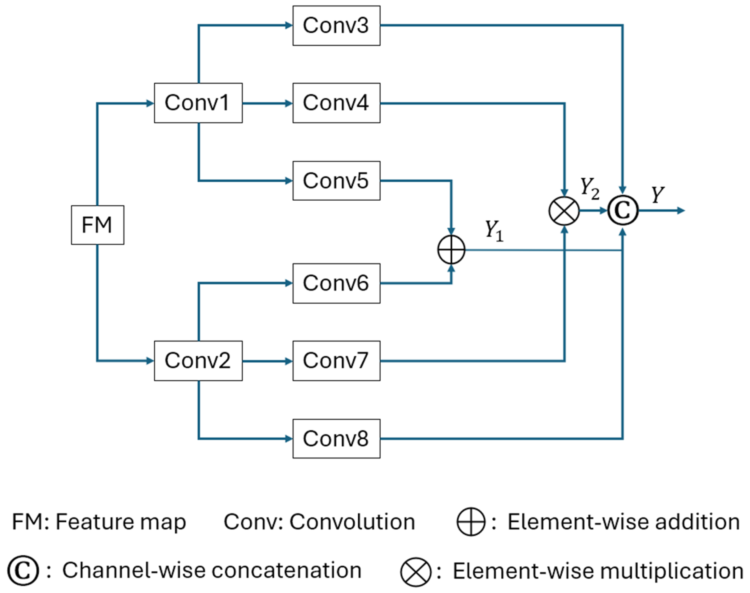
This proposed module (Figure 3) autonomously adapts multi-domains for multi-task problems by re-arranging the weights’ positions and their amplitudes using element-wise addition and element-wise multiplication, respectively. The input feature map (FM) has been exploited in multi-stage/multi-level mood to consider novel features for self-adaptation and thereby compensate for small training data and mitigate the inter-task variability. All the convolutions used in this module have same dimension, dilation, and stride. They were particularly used correcting the weights position to accurately fit the salient features in the input. For example, Conv5 and Conv6 in Figure 3 aggregate the input and then translate those weights to the correct positions by iterative process in the model training. Furthermore, the features’ amplitude was enhanced by scaling the features to mitigate the features vanishing through the depth of the model. For example, Conv4 and Conv7 enhanced the output features by scaling. The position-corrected and enhanced features were concatenated with the original features to preserve the originality of the features. Overall, this proposed module generates self-corrected and adapted novel tensors and, therefore, assists the blind-FSL. The self-adapted features (concerning position and amplitude) were concatenated channel-wise with the original features to preserve the originality of the eigenvalues. A standard representation for convolution is shown in Equation (4), and the mathematical modeling for the SMDA module is expressed in Equations (4)–(7) as follows:
C o n v ( . ) m , n ,   F M = j = 1 J k = 1 K F M j , k . ω m j ,   n k + b
Y 1 = C o n v 5 C o n v 1 F M     C o n v 6 C o n v 2 F M
Y 2 = C o n v 4 C o n v 1 F M     C o n v 7 C o n v 2 F M
Y = C o n v 3 C o n v 1 F M   ©   C o n v 8 C o n v 2 F M   ©   Y 1   ©   Y 2
where Conv(.) denotes the convolutional operation and Y1, Y2, and Y indicate positional corrected weights, enhanced amplitudes, and output of the SMDA module, respectively. m and n denote the vertical and horizontal dimensions of the convolutional kernel, j and k are the translating indices, and b is the bias component.

2.4. Inter-Function Discriminator (IFD)

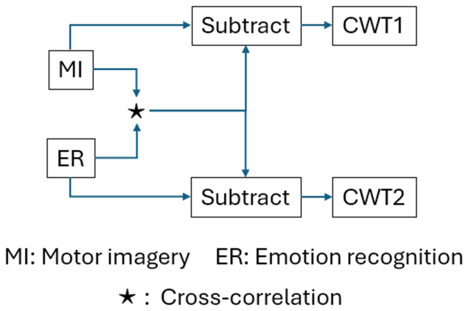
The proposed IFD module (Figure 4) removes common features by extracting similarity between each pair of multi-task classes using cross-correlation, then subtracts those common features from both tasks to emphasize the distinctive features for each task. This encourages the model to learn task-distinctive features and overcome overfitting by mitigating common features. Specifically, this module enhances inter-functional features discrimination to overcome the misleading learning of the proposed model on common features. The MI and ER (it can be any pair among MI, ER, and SS) were cross-correlated to exploit the common features. These common features are then subtracted from the corresponding input task to ensure the feature discrimination. These discriminated features are then transformed by cwt to obtain a TFR. This module can be expressed mathematically in Equations (8) and (9) as follows:
P 1 = C W T 1 ( M I M I E R )
P 2 = C W T 2 ( E R M I E R )

2.5. Holistic-Local Fusion (HLF) Module

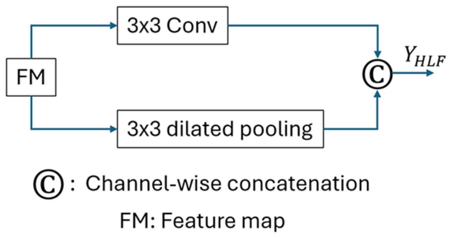
This proposed module is shown in Figure 5. FM has been exploited using a convolution with a small kernel to preserve detailed features by exploiting locally equivariant features. This assists the model in learning causal and non-causal features of each task. Moreover, the dilated-pooling operation exploits contextual-invariant features to learn corresponding scaled features of each task to mitigate unnecessary variabilities in each task. Both transformations were concatenated channel-wise. Particularly, the features vary intensively across datasets, which makes it difficult to decide the size of the convolution kernel. Considering a small kernel can exploit detailed features that could accurately aggregate one task but could not another due to the scale variations across the tasks. Therefore, we utilized a small-kernel convolution layer to exploit local-equivariant features and dilated pooling layer to exploit contextual-invariant features. Consequently, this module assists the multifunctionality by learning causal/non-causal and scaled-varying features to adapt all the tasks. This module is expressed mathematically in Equation (10) as follows:
Y H L F = j = 1 J k = 1 K F M j , k . ω m j ,   n k + b   ©   1 N M i = 1 N j = 1 M F M ( i + 3 , j + 3 )
where m and n denote the vertical and horizontal dimensions of the convolutional kernel, j and k are the translating indices, and b is the bias component.

2.6. FDE

Fractals are complex structures defined by self-similarity and deviation from conventional geometric patterns [43]. The fractal dimension (FD) serves as a quantitative metric for evaluating such complexity by describing how spatially concentrated or dispersed a shape is. In this study, FDE is performed on binary images derived from gradient-class activation map (Grad-CAM) activation regions extracted from CWT scalograms generated using EEG signals collected during LMI and RMI. The resulting FD values, typically ranging from 1 to 2, indicate the structural complexity of the corresponding binary class activation maps, with higher values reflecting more intricate and irregular patterns.
In our study, FD is calculated using a simple box-counting method [44,45] with binary image only by the central processing unit (CPU) without an additional GPU card in a CUDA environment, as shown in Equation (11). FDE can be used in various other recent fields for complexity examination, such as biomedical volume rendering optimization [46], fractal analysis of climate dynamics trend [47], and ultra-fast computation for RGB using fractal dimension [48]. Although they showed high accuracies for FDE, their computational loads are too much to be applied to our task due to 3D FDE [46] and FDE in sequences [47]. In addition, although the method [48] is computationally effective, it requires additional graphics processing unit (GPU) card of high computational power in a compute unified device architecture (CUDA) environment, which is also difficult to be applied to our task. Here, M denotes the number of boxes needed to cover the activated region and r is the scale factor.
F D = lim r 0 l o g ( M ( r ) ) l o g ( 1 / r )
The FD lies within the interval 1 ≤ FD ≤ 2, and for each scale r   > 0, there exists a corresponding box count M ( r ). The detailed procedure for FDE of Grad-CAM-based activation regions using the box-counting method is described in Algorithm 1.
Algorithm 1 Pseudocode for FDE and training of the proposed model
Input: Biscalo: Binary class activation map extracted from scalogram, MI, ER, SS.
Output: FD: Fractal dimension, trained weights’ matrix (W).
1: Find the largest dimension and round it up to the closest power of two.
 Max_dim = max(size(Biscalo))
    M = 2[log2(Max_dim)]
2: Ensure the image is padded to match r if its original size is insufficient.
   if size(Biscalo) < size( r )
      Pad_wid=((0, r −Biscalo.shape [0]), (0, r −Biscalo.shape [1]))
      Pad_Biscalo=padding(Biscalo, Pad_wid, mode=‘constant’, constant_values=0)
   else
      Pad_Biscalo=Biscalo
3: Create an array to store the number of boxes at each scale level.
n = zeros(1, r +1)
4: Count the number of boxes at scale r that overlap with any active (positive) region.
n[ r +1]=sum(Biscalo[:])
5: While r >1:
    a. Divide r by 2 to reduce its scale.
    b. Replace M ( r ) with the newly computed value.
6: Calculate log( M ( r ) ) and log( 1 / r ) for every scale r.
7: Apply linear regression to the log–log data points.
8: FD corresponds to the gradient of the best-fit line in the log–log space.
Return FD
9: Training the proposed model
 CWT=MMSE(MI, ER, SS)
 CWT=IFD(MI, ER)
 SMDA= φ 1 ( C W T )
 HLF= φ 2 ( C W T )         φ ( . ) : intermediate learnables.
return W.

3. Experiments and Results

3.1. Experimental Data

We utilized three open datasets to evaluate our proposed model; their descriptions are as follows.

3.1.1. Brain Computer Interface (BCI) Competition IV-2a [49] (Dataset I)

This is a public dataset, recording EEG data from nine healthy volunteers at a 250 Hz sampling rate for training and testing sessions on different days. Imaginations for the left hand (LH), the right hand (RH), the foot, and the tongue were recorded. We considered LH and RH from this MI dataset. Each subject (volunteer) performed six runs per session and twelve trials per task. Therefore, each subject performed 144 trials per session and 288 trials per two sessions. The training subjects in this dataset are shown as [A01T, A02T, …, A09T] and the evaluation subjects are denoted as [A01E, A02E, …, A09E]. This dataset has been widely used for biological signal-based previous research [50].

3.1.2. DREAMER Dataset [51] (Dataset II)

This is a multimodal public dataset used to detect emotion recognition classes, i.e., valence and arousal, in this paper. The ECG and EEG signals were recorded from 23 participants (14 males and 9 females), watching 18 film clips while they wore wireless off-the-shelf low-cost equipment for affective computing. The clip length ranged between 65 and 393 s. The EEG data was recorded from 14 electrodes at 128 Hz sampling rate. The valence, arousal, and dominance were acquired by self-assessment manikins.

3.1.3. Sleep-EDF Database Expanded [52] (Dataset III)

This is a public physioNet dataset used to classify N1 and N2 sleep stages in this paper. Eight Caucasians recorded the data at a sampling rate of 100 Hz. In this study, every 30 s of the EEG signal is called one epoch.
We used MATLAB 2024a [53], a desktop computer with specifications including an NVIDIA GTX 1070 GPU card of low computational power [54], an Intel® Core™ i7-3770K CPU, and 16 GB RAM for model designing, training, and evaluation. An adaptive moment estimation optimizer [55] has been used as a parameter optimizer. The number of epochs and initial learning rate were set to 50 and 10−3. The mini-batch size was set equal to the corresponding shot.

3.2. Ablation Study

We performed an ablation study (Table 1) to evaluate the contribution of each proposed module. Each proposed module enhanced the detection accuracy of multitasks. We performed the ablation study by adding each proposed module gradually, but there could be many combinations of the proposed modules, which exploration can lengthen this paper. Each proposed module remarkably enhances the detection accuracy of the underlying problem, which shows their effectiveness for the desired operation. Specifically, the SMDA and HLF modules contribute significantly compared to other modules, as shown in Table 1. This shows good self-corrected and enhanced features decoding performance for the SMDA module, and excellent adaptability of the variable-scaled features of the underlying multi-task problem. Although the inclusion of each proposed module enhances the detection accuracy of the multitask problem, it increases the computational cost of the proposed model, i.e., the number of parameters is 27.8 million, and the inference time is 34.2 ms.

3.3. Comparison with SOTA Methods

3.3.1. Based on a Single Dataset (Individual Task)

We performed 1-shot, 5-shot, 10-shot, and 20-shot for each MI, ER, and SS tasks and compared with SOTA methods. Regarding MI detection, our proposed algorithm outperformed all SOTA methods except Meta-L MI [15] and FSL-DA MI [16] using 5-shot learning. This could be due to their well-customized feature extraction capabilities for 5-shot learning. Furthermore, our proposed model outperformed all SOTA methods except MAML + ResNet-18 [24] for ER detection using 1-shot learning. This shows a better-organized model architecture, which can better extract the target features from 1 training sample than our proposed model. For SS detection, our proposed model outperformed SOTA methods except XSleepNet [35] using 20-shot learning. This could be due to its better optimization on global features than our proposed model.
Some of the insights regarding Table 2 are as follows: a remarkable increase (with increasing training data) in detection accuracy was observed for IFSL-MI [13], EEG-CNN [56], MI-SCNN [57], MI-HFDNN [58], CFE-FSL MI [18], SVM [25], MetaSleepLearner [30], DeepSleepNet [32], AttnSleep [34], XSleepNet [35], and Multi-BioSig-Net (proposed). These models could have mitigated underfitting and overfitting and show an adaptable decoding performance for limited and increased training data. Other SOTA methods, including Meta-L MI [15], FSL-DA MI [16], MI RelationNet [1], SleepEEGNet [31], and DeepSleepNet-Lite [33], increase accuracy with increasing training data, and a saturation could be observed for 20-shot learning. This could be due to overfitting on local features of those models. EEGNet [26] slowly increased the accuracy for 1- and 5-shot learning compared to 10- and 2-shot learning. This could be due to underfitting using few training samples.

3.3.2. Based on a Combined Dataset (Multi-Task)

We trained our proposed model by taking 1, 5, 10, and 20 training samples (s) from MI, ER, and SS (we called it a combined dataset). The SOTA models customized for MI in Table 3, outperformed ER and SS for all shots, and it is also valid for model customization for ER and SS. Some of the insights in Table 3 are as follows. The SOTA models EEG-CNN [56], EEGNet [26], and XSleepNet [35] have a better performance on the combined dataset than on the dataset they were customized for. This might be due to their generalizability for global variability instead of customized variability. The remaining SOTA methods have declined performance on the combined dataset than the individual one. This could be due to overfitting caused by optimization on local optima initiated by various datasets variability. Our proposed model outperformed all the SOTA models except XSleepNet [35] for 10 and 20 shots. The second best is the SOTA model, named as XSleepNet [35]. Various SOTA models, i.e., Meta-L MI [15], MI RelationNet [1], EEG-CNN [56], SVM [25], MetaSleepLearner [30], DeepSleepNet [32], and DeepSleepNet-Lite [33] decreased the rate of increasing accuracy while adding training data. This might be due to their affinity to data similarity which causes overfitting when extracting abundant similarity.
The parameters’ count (P) and inference time (IT) in Table 2 and Table 3 show the model size and the algorithm’s speed during testing of a sample for practical applications. Some SOTA algorithms have very large P and IT comparatively, such as Meta-L MI [15], FSL-DA MI [16], and MI RelationNet [1]. This could be due to the utilization of fully connected layers in their model to ensure performance enhancement. Others SOTA have very low P and small IT comparatively, such as Average Ensemble [36], DeepSleepNet-Lite [33], XSleepNet [35], SleepEEGNet [31], MetaSleepLearner [30], EEGNet [26], and EEG-CNN [56]. The reason might be due to the parameter quantization and utilization of dilation to make the model light for edge applications. Our proposed Multi-BioSig-Net model has P of 27.8 million and IT of 34.2 ms, which increases these factors slightly to ensure the model performs well for multi-tasking.
Although there are previous studies of single tasking biological signal classification without FSL [25,26,31,32,33,36,56,57,58] and single tasking biological signal classification with FSL [1,13,15,16,18,24,30], there is no previous research to perform multitasking biological signal classification using blind-FSL like our proposed method. Generally, SOTA algorithms perform well on the datasets that they are customized for. For instance, the algorithms [1,13,15,16,57,58] are designed for MI task; therefore, they outperformed other tasks due to their customized characteristics. Similarly, the algorithms [25,26] are designed for ER task, which outperformed MI and SS tasks. The algorithms [30,31,32,33,36,56] are designed for SS task and, therefore, outperformed MI and ER tasks. The algorithms non-customized for a task usually underperform in the customized algorithms due to the incompatibility of the optimal parameters with the task characteristics.

4. Discussion

4.1. Results of FDE

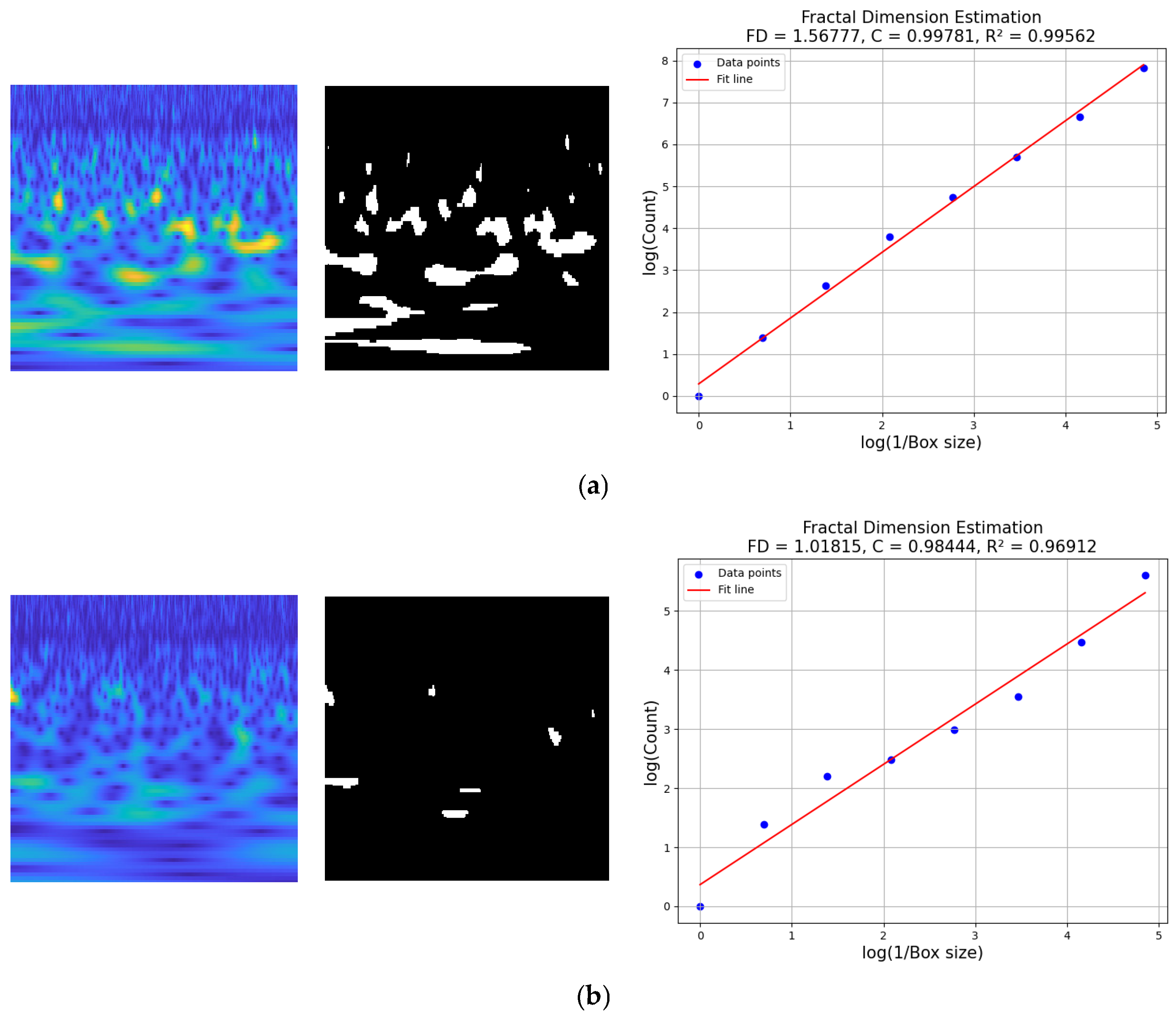
To evaluate the complexity of Grad-CAM activation regions derived from the EEG-based scalograms, we estimated the FD using the box-counting method as described in Section 2.6. Table 4 presents the FD values for LMI and RMI, along with the corresponding regression coefficients (C) and determination coefficients (R2), as shown in Figure 6.
The FD value for the LMI condition (as shown in Figure 6a) was substantially higher (1.56777) than that of the RMI condition (1.01815), indicating that the activation region under the LMI condition exhibits greater structural complexity and irregularity. This suggests that the neural response pattern captured during LMI is more spatially distributed or fragmented, as reflected by the more intricate texture of the corresponding binary activation map. In contrast, the lower FD observed for the RMI condition (as shown in Figure 6b) suggests a more spatially compact and less complex activation region. This may imply that the RMI induced more localized and concentrated responses in the Grad-CAM heatmap. By achieving high coefficients of determination (R2) in the log–log regression analysis, strong reliability of the fitting was ensured. This confirms that the FD serves as a robust quantitative metric for clearly distinguishing structural complexity differences between LMI and RMI, and our extracted features are effective for the discrimination of LMI and RMI. In our study, FDE is simply used to evaluate the differences in features of LMI/RMI by scalogram in terms of structural similarity metric, and FDE is not integrated into the overall system. Therefore, there is no relationship with modules, and it does not have any impact on overall performance.

4.2. Statistical Evaluation

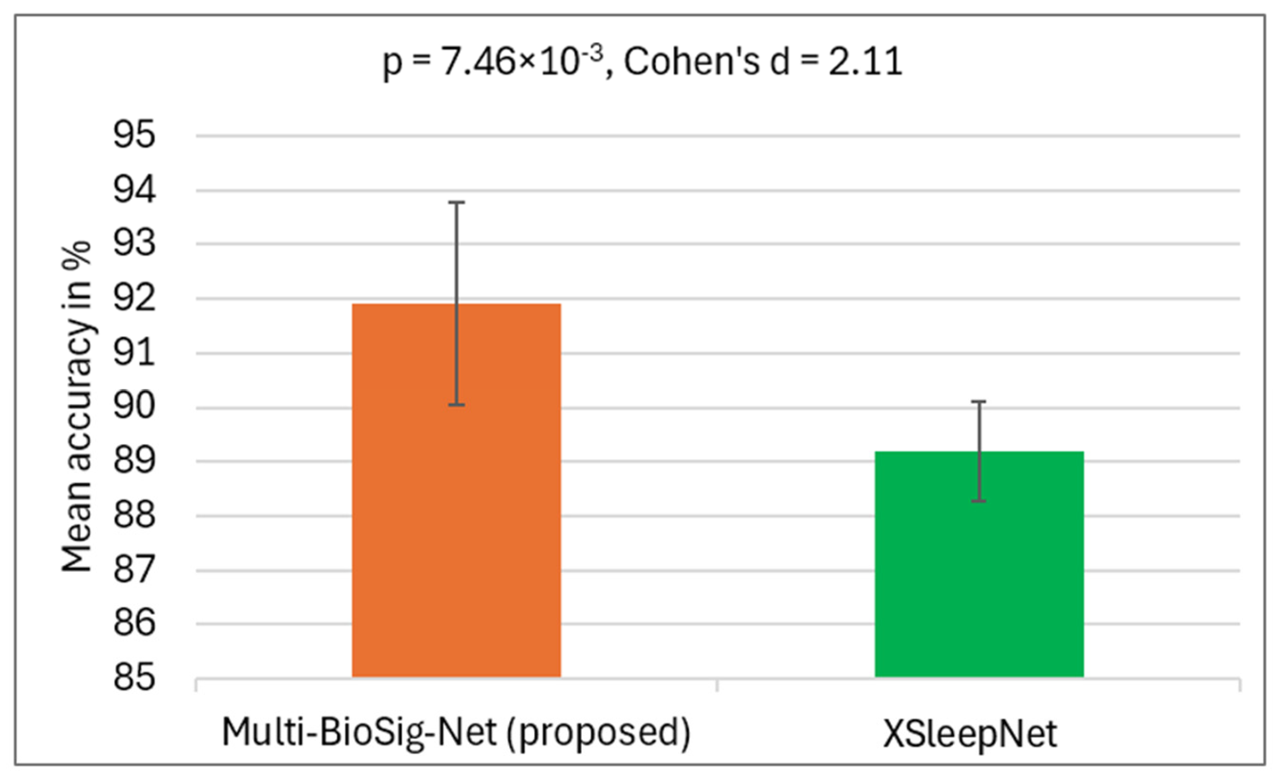
We evaluated the significance of our proposed model using Student’s t-test [59] and Cohen’s d [60]. Their values were 7.46 × 10⁻³ and 2.11, respectively, as shown in Figure 7. We considered the accuracy of SS for 20-shot due to its highest significance among others. The second-best model for the SS 20-shot is XSleepNet [35], as shown in Table 3. The results show that the proposed model has a significant difference at a significance level of 99%. The large Cohen’s d value (2.11) shows that both the compared models have distinct behaviors toward the same dataset, and the one with the larger mean value (proposed model) dominates the other (second-best model).

4.3. Training Loss-Accuracy Graph

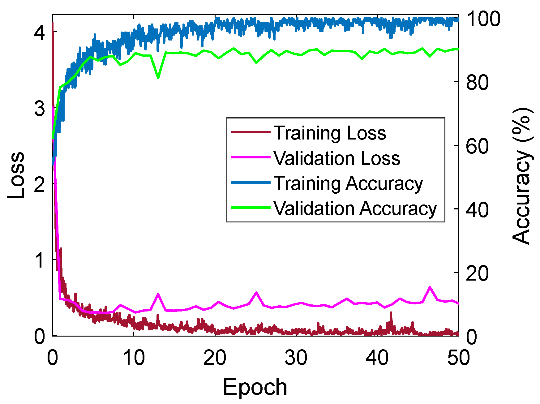
The training and validation accuracy-loss graphs for the proposed model are shown in Figure 8. The graphs of training loss and accuracy are converged according to the increment of epoch, confirming that our model was sufficiently trained with training data. In addition, the graphs of validation loss and accuracy are converged according to the increment of epoch, confirming that our model was not overfitted to training data.

5. Conclusions

This paper addressed challenges such as intra- and inter-task variabilities in biological signals caused by individual biological differences. Furthermore, a novel blind FSL was proposed, which does not need any pretrained model for target task prediction. A few modules were proposed, i.e., MMSE, SMDA, IFD, and HLF, to emphasize multimodal common features for model’s robustness on few-shot learning, self-correct the weights’ position and amplitude to detect the individual task accurately, to discriminate inter-task features to mitigate model’s overfitting on minima of other tasks, and adapt the variable scale of all the tasks for accurate detection of multi tasks. Using these modules, the proposed Multi-BioSig-Net accurately detected various tasks, i.e., MI, ER, and SS, using individual and combined datasets. The advancement of the proposed model was evaluated statistically using Student’s t-test. In addition, FDE was employed for the classification of LMI and RMI, confirming that proposed method can effectively extract the discriminative features for this task. Moreover, the stability of the proposed model was good for the combined dataset (as shown in Table 3), but the limitation of the proposed model is underperforming for different tasks based on 1-, 5-, and 20-shot, as shown in Table 2. This shows an unstable behavior towards the task variability when the training shot is changing.
This limitation would be addressed in the future by proposing a generalized decoder for biological signals. In addition, the multi-task domain will be expanded in the future.

Author Contributions

Conceptualization, N.U.; methodology, N.U.; data curation, S.G.K. and J.S.K.; validation, M.S.J.; supervision, K.R.P.; writing—original draft preparation, N.U.; writing—review and editing, K.R.P. All authors have read and agreed to the published version of the manuscript.

Funding

This research was supported by the Ministry of Science and ICT (MSIT), Korea, under the Information Technology Research Center (ITRC) support program (IITP-2025-RS-2020-II201789) and by the Artificial Intelligence Convergence Innovation Human Resources Development (IITP-2025-RS-2023-00254592) supervised by the Institute of Information & Communications Technology Planning & Evaluation (IITP).

Data Availability Statement

The data supporting the findings of this study are available from the corresponding author (K. R. Park) upon request.

Conflicts of Interest

The authors declare no conflicts of interest.

References

  1. An, S.; Kim, S.; Chikontwe, P.; Park, S.H. Dual Attention Relation Network With Fine-Tuning for Few-Shot EEG Motor Imagery Classification. IEEE Trans. Neural Netw. Learn. Syst. 2024, 35, 15479–15493. [Google Scholar] [CrossRef] [PubMed]
  2. Ullah, N.; Mahmood, T.; Kim, S.G.; Nam, S.H.; Sultan, H.; Park, K.R. DCDA-Net: Dual-Convolutional Dual-Attention Network for Obstructive Sleep Apnea Diagnosis from Single-Lead Electrocardiograms. Eng. Appl. Artif. Intell. 2023, 123, 106451. [Google Scholar] [CrossRef]
  3. Zhang, T.; Ali, A.E.; Hanjalic, A.; Cesar, P. Few-Shot Learning for Fine-Grained Emotion Recognition Using Physiological Signals. IEEE Trans. Multimed. 2023, 25, 3773–3787. [Google Scholar] [CrossRef]
  4. Sannino, G.; De Pietro, G. A Deep Learning Approach for ECG-Based Heartbeat Classification for Arrhythmia Detection. Future Gener. Comput. Syst. 2018, 86, 446–455. [Google Scholar] [CrossRef]
  5. Yılmaz, B.; Asyalı, M.H.; Arıkan, E.; Yetkin, S.; Özgen, F. Sleep Stage and Obstructive Apneaic Epoch Classification Using Single-Lead ECG. BioMed. Eng. OnLine 2010, 9, 39. [Google Scholar] [CrossRef]
  6. Amin, S.U.; Altaheri, H.; Muhammad, G.; Abdul, W.; Alsulaiman, M. Attention-Inception and Long- Short-Term Memory-Based Electroencephalography Classification for Motor Imagery Tasks in Rehabilitation. IEEE Trans. Ind. Inform. 2022, 18, 5412–5421. [Google Scholar] [CrossRef]
  7. Bang, J.-S.; Lee, M.-H.; Fazli, S.; Guan, C.; Lee, S.-W. Spatio-Spectral Feature Representation for Motor Imagery Classification Using Convolutional Neural Networks. IEEE Trans. Neural Netw. Learn. Syst. 2022, 33, 3038–3049. [Google Scholar] [CrossRef]
  8. Hsu, W.Y.; Cheng, Y.W. EEG-Channel-Temporal-Spectral-Attention Correlation for Motor Imagery EEG Classification. IEEE Trans. Neural Syst. Rehabil. Eng. 2023, 31, 1659–1669. [Google Scholar] [CrossRef]
  9. Joshi, V.M.; Ghongade, R.B. EEG Based Emotion Detection Using Fourth Order Spectral Moment and Deep Learning. Biomed. Signal Process. Control 2021, 68, 102755. [Google Scholar] [CrossRef]
  10. Ozdemir, M.A.; Degirmenci, M.; Izci, E.; Akan, A. EEG-Based Emotion Recognition with Deep Convolutional Neural Networks. Biomed. Eng. Biomed. Tech. 2021, 66, 43–57. [Google Scholar] [CrossRef] [PubMed]
  11. Rodriguez Aguiñaga, A.; Muñoz Delgado, L.; López-López, V.R.; Calvillo Téllez, A. EEG-Based Emotion Recognition Using Deep Learning and M3GP. Appl. Sci. 2022, 12, 2527. [Google Scholar] [CrossRef]
  12. Liang, X.; Tu, G.; Du, J.; Xu, R. Multi-Modal Attentive Prompt Learning for Few-Shot Emotion Recognition in Conversations. J. Artif. Intell. Res. 2024, 79, 825–863. [Google Scholar] [CrossRef]
  13. She, Q.; Li, C.; Tan, T.; Fang, F.; Zhang, Y. Improved Few-Shot Learning Based on Triplet Metric for Motor Imagery EEG Classification. IEEE Trans. Cogn. Dev. Syst. 2025, 17, 987–999. [Google Scholar] [CrossRef]
  14. Tang, M.; Zhang, Z.; He, Z.; Li, W.; Mou, X.; Du, L.; Wang, P.; Zhao, Z.; Chen, X.; Li, X.; et al. Deep Adaptation Network for Subject-Specific Sleep Stage Classification Based on a Single-Lead ECG. Biomed. Signal Process. Control 2022, 75, 103548. [Google Scholar] [CrossRef]
  15. Yu, J.; Duan, L.; Ji, H.; Li, J.; Pang, Z. Meta-Learning for EEG Motor Imagery Classification. Comput. Inform. 2024, 43, 735–755. [Google Scholar] [CrossRef]
  16. Phunruangsakao, C.; Achanccaray, D.; Hayashibe, M. Deep Adversarial Domain Adaptation With Few-Shot Learning for Motor-Imagery Brain-Computer Interface. IEEE Access 2022, 10, 57255–57265. [Google Scholar] [CrossRef]
  17. Chen, L.; Yu, Z.; Yang, J. SPD-CNN: A Plain CNN-Based Model Using the Symmetric Positive Definite Matrices for Cross-Subject EEG Classification with Meta-Transfer-Learning. Front. Neurorobot. 2022, 16, 958052. [Google Scholar] [CrossRef]
  18. Zhu, L.; Liu, Y.; Liu, R.; Peng, Y.; Cao, J.; Li, J.; Kong, W. Decoding Multi-Brain Motor Imagery From EEG Using Coupling Feature Extraction and Few-Shot Learning. IEEE Trans. Neural Syst. Rehabil. Eng. 2023, 31, 4683–4692. [Google Scholar] [CrossRef]
  19. Liu, W.; Qiu, J.-L.; Zheng, W.-L.; Lu, B.-L. Comparing Recognition Performance and Robustness of Multimodal Deep Learning Models for Multimodal Emotion Recognition. IEEE Trans. Cogn. Dev. Syst. 2022, 14, 715–729. [Google Scholar] [CrossRef]
  20. Cheng, J.; Chen, M.; Li, C.; Liu, Y.; Song, R.; Liu, A.; Chen, X. Emotion Recognition From Multi-Channel EEG via Deep Forest. IEEE J. Biomed. Health Inform. 2021, 25, 453–464. [Google Scholar] [CrossRef]
  21. Cui, H.; Liu, A.; Zhang, X.; Chen, X.; Wang, K.; Chen, X. EEG-Based Emotion Recognition Using an End-to-End Regional-Asymmetric Convolutional Neural Network. Knowl.-Based Syst. 2020, 205, 106243. [Google Scholar] [CrossRef]
  22. Quan, J.; Li, Y.; Wang, L.; He, R.; Yang, S.; Guo, L. EEG-Based Cross-Subject Emotion Recognition Using Multi-Source Domain Transfer Learning. Biomed. Signal Process. Control 2023, 84, 104741. [Google Scholar] [CrossRef]
  23. Liu, Y.; Ding, Y.; Li, C.; Cheng, J.; Song, R.; Wan, F.; Chen, X. Multi-Channel EEG-Based Emotion Recognition via a Multi-Level Features Guided Capsule Network. Comput. Biol. Med. 2020, 123, 103927. [Google Scholar] [CrossRef]
  24. Chen, C.; Fang, H.; Yang, Y.; Zhou, Y. Model-Agnostic Meta-Learning for EEG-Based Inter-Subject Emotion Recognition. J. Neural Eng. 2025, 22, 016008. [Google Scholar] [CrossRef]
  25. Zheng, W.-L.; Lu, B.-L. Investigating Critical Frequency Bands and Channels for EEG-Based Emotion Recognition with Deep Neural Networks. IEEE Trans. Auton. Ment. Dev. 2015, 7, 162–175. [Google Scholar] [CrossRef]
  26. Lawhern, V.J.; Solon, A.J.; Waytowich, N.R.; Gordon, S.M.; Hung, C.P.; Lance, B.J. EEGNet: A Compact Convolutional Neural Network for EEG-Based Brain–Computer Interfaces. J. Neural Eng. 2018, 15, 056013. [Google Scholar] [CrossRef]
  27. Sangineto, E.; Zen, G.; Ricci, E.; Sebe, N. We Are Not All Equal: Personalizing Models for Facial Expression Analysis with Transductive Parameter Transfer. In Proceedings of the 22nd ACM International Conference on Multimedia, Orlando, FL, USA, 3 November 2014; pp. 357–366. [Google Scholar]
  28. Pan, S.J.; Tsang, I.W.; Kwok, J.T.; Yang, Q. Domain Adaptation via Transfer Component Analysis. IEEE Trans. Neural Netw. 2011, 22, 199–210. [Google Scholar] [CrossRef]
  29. Müller, K.-R.; Mika, S.; Tsuda, K.; Schölkopf, K. An Introduction to Kernel-Based Learning Algorithms. In Handbook of Neural Network Signal Processing; CRC Press: Boca Raton, FL, USA, 2002; ISBN 978-1-315-22041-3. [Google Scholar]
  30. Banluesombatkul, N.; Ouppaphan, P.; Leelaarporn, P.; Lakhan, P.; Chaitusaney, B.; Jaimchariyatam, N.; Chuangsuwanich, E.; Chen, W.; Phan, H.; Dilokthanakul, N.; et al. MetaSleepLearner: A Pilot Study on Fast Adaptation of Bio-Signals-Based Sleep Stage Classifier to New Individual Subject Using Meta-Learning. IEEE J. Biomed. Health Inform. 2021, 25, 1949–1963. [Google Scholar] [CrossRef]
  31. Mousavi, S.; Afghah, F.; Acharya, U.R. SleepEEGNet: Automated Sleep Stage Scoring with Sequence to Sequence Deep Learning Approach. PLoS ONE 2019, 14, e0216456. [Google Scholar] [CrossRef]
  32. Supratak, A.; Dong, H.; Wu, C.; Guo, Y. DeepSleepNet: A Model for Automatic Sleep Stage Scoring Based on Raw Single-Channel EEG. IEEE Trans. Neural Syst. Rehabil. Eng. 2017, 25, 1998–2008. [Google Scholar] [CrossRef]
  33. Fiorillo, L.; Favaro, P.; Faraci, F.D. DeepSleepNet-Lite: A Simplified Automatic Sleep Stage Scoring Model With Uncertainty Estimates. IEEE Trans. Neural Syst. Rehabil. Eng. 2021, 29, 2076–2085. [Google Scholar] [CrossRef] [PubMed]
  34. Eldele, E.; Chen, Z.; Liu, C.; Wu, M.; Kwoh, C.-K.; Li, X.; Guan, C. An Attention-Based Deep Learning Approach for Sleep Stage Classification With Single-Channel EEG. IEEE Trans. Neural Syst. Rehabil. Eng. 2021, 29, 809–818. [Google Scholar] [CrossRef] [PubMed]
  35. Phan, H.; Chén, O.Y.; Tran, M.C.; Koch, P.; Mertins, A.; De Vos, M. XSleepNet: Multi-View Sequential Model for Automatic Sleep Staging. IEEE Trans. Pattern Anal. Mach. Intell. 2022, 44, 5903–5915. [Google Scholar] [CrossRef] [PubMed]
  36. Khalili, E.; Mohammadzadeh Asl, B. Automatic Sleep Stage Classification Using Temporal Convolutional Neural Network and New Data Augmentation Technique from Raw Single-Channel EEG. Comput. Methods Programs Biomed. 2021, 204, 106063. [Google Scholar] [CrossRef]
  37. Perslev, M.; Darkner, S.; Kempfner, L.; Nikolic, M.; Jennum, P.J.; Igel, C. U-Sleep: Resilient High-Frequency Sleep Staging. NPJ Digit. Med. 2021, 4, 72. [Google Scholar] [CrossRef]
  38. Goshtasbi, N.; Boostani, R.; Sanei, S. SleepFCN: A Fully Convolutional Deep Learning Framework for Sleep Stage Classification Using Single-Channel Electroencephalograms. IEEE Trans. Neural Syst. Rehabil. Eng. 2022, 30, 2088–2096. [Google Scholar] [CrossRef]
  39. Qu, W.; Wang, Z.; Hong, H.; Chi, Z.; Feng, D.D.; Grunstein, R.; Gordon, C. A Residual Based Attention Model for EEG Based Sleep Staging. IEEE J. Biomed. Health Inform. 2020, 24, 2833–2843. [Google Scholar] [CrossRef]
  40. Seo, H.; Back, S.; Lee, S.; Park, D.; Kim, T.; Lee, K. Intra- and Inter-Epoch Temporal Context Network (IITNet) Using Sub-Epoch Features for Automatic Sleep Scoring on Raw Single-Channel EEG. Biomed. Signal Process. Control 2020, 61, 102037. [Google Scholar] [CrossRef]
  41. Li, J.; Wu, C.; Pan, J.; Wang, F. Few-Shot EEG Sleep Staging Based on Transductive Prototype Optimization Network. Front. Neuroinform. 2023, 17, 1297874. [Google Scholar] [CrossRef]
  42. Torrence, C.; Compo, G.P. A Practical Guide to Wavelet Analysis. Bull. Am. Meteorol. Soc. 1998, 79, 61–78. [Google Scholar] [CrossRef]
  43. Brouty, X.; Garcin, M. Fractal properties; information theory, and market efficiency. Chaos Solitons Fractals 2024, 180, 114543. [Google Scholar] [CrossRef]
  44. Yin, J. Dynamical fractal: Theory and case study. Chaos Solitons Fractals 2023, 176, 114190. [Google Scholar] [CrossRef]
  45. Crownover, R.M. Introduction to Fractals and Chaos, 1st ed.; Jones & Bartlett Publisher: Burlington, MA, USA, 1995. [Google Scholar]
  46. Denisova, E.; Bocchi, L. Optimizing Biomedical Volume Rendering: Fractal Dimension-Based Approach for Enhanced Performance. In Proceedings of the Medical Imaging 2024: Clinical and Biomedical Imaging, San Diego, CA, USA, 2 April 2024; SPIE: Bellingham, WA, USA, 2024; Volume 12930, pp. 640–649. [Google Scholar]
  47. Meenakshi, M.; Gowrisankar, A. Fractal-Based Approach on Analyzing the Trends of Climate Dynamics. Int. J. Mod. Phys. B 2024, 38, 2440006. [Google Scholar] [CrossRef]
  48. Ruiz de Miras, J.; Li, Y.; León, A.; Arroyo, G.; López, L.; Torres, J.C.; Martín, D. Ultra-Fast Computation of Fractal Dimension for RGB Images. Pattern Anal. Applic. 2025, 28, 36. [Google Scholar] [CrossRef]
  49. Brunner, C.; Leeb, R.; Muller-Putz, G.R.; Schlogl, A. BCI Competition 2008—Graz Data Set A; Institute for Knowledge Discovery, Graz University of Technology: Graz, Austria. Available online: http://www.bbci.de/competition/iv/desc_2a.pdf (accessed on 29 August 2025).
  50. Ullah, N.; Sultan, H.; Hong, J.S.; Kim, S.G.; Akram, R.; Park, K.R. Convolutional Self-Attention with Adaptive Channel-Attention Network for Obstructive Sleep Apnea Detection Using Limited Training Data. Eng. Appl. Artif. Intell. 2025, 156, 111154. [Google Scholar] [CrossRef]
  51. Katsigiannis, S.; Ramzan, N. DREAMER: A Database for Emotion Recognition Through EEG and ECG Signals from Wireless Low-Cost Off-the-Shelf Devices. IEEE J. Biomed. Health Inform. 2018, 22, 98–107. [Google Scholar] [CrossRef]
  52. Kemp, B.; Zwinderman, A.; Tuk, B.; Kamphuisen, H.; Oberyé, J. The Sleep-EDF Database [Expanded]. PhysioNet, MIT Laboratory for Computational Physiology: Cambridge, MA, USA, 2018. [Google Scholar] [CrossRef]
  53. MATLAB R2024a. 2025. Available online: https://www.mathworks.com/products/matlab.html (accessed on 17 April 2025).
  54. GeForce GTX 1070. 2025. Available online: https://www.nvidia.com/en-gb/geforce/products/10series/geforce-gtx-1070/ (accessed on 17 April 2025).
  55. Kingma, D.P.; Ba, J. Adam: A Method for Stochastic Optimization. arXiv 2017, arXiv:1412.6980. [Google Scholar] [CrossRef]
  56. Schirrmeister, R.T.; Springenberg, J.T.; Fiederer, L.D.J.; Glasstetter, M.; Eggensperger, K.; Tangermann, M.; Hutter, F.; Burgard, W.; Ball, T. Deep Learning with Convolutional Neural Networks for EEG Decoding and Visualization. Hum. Brain Mapp. 2017, 38, 5391–5420. [Google Scholar] [CrossRef]
  57. Kashefi Amiri, H.; Zarei, M.; Daliri, M.R. Motor Imagery Electroencephalography Channel Selection Based on Deep Learning: A Shallow Convolutional Neural Network. Eng. Appl. Artif. Intell. 2024, 136, 108879. [Google Scholar] [CrossRef]
  58. Sorkhi, M.; Jahed-Motlagh, M.R.; Minaei-Bidgoli, B.; Daliri, M.R. Hybrid Fuzzy Deep Neural Network toward Temporal-Spatial-Frequency Features Learning of Motor Imagery Signals. Sci. Rep. 2022, 12, 22334. [Google Scholar] [CrossRef]
  59. Student’s t-test. 15 June 2025. Available online: https://en.wikipedia.org/w/index.php?title=Student%27s_t-test&oldid=1262286726 (accessed on 25 June 2025).
  60. Cohen, J. A power primer. Psychol. Bull. 1992, 112, 155–159. [Google Scholar] [CrossRef]
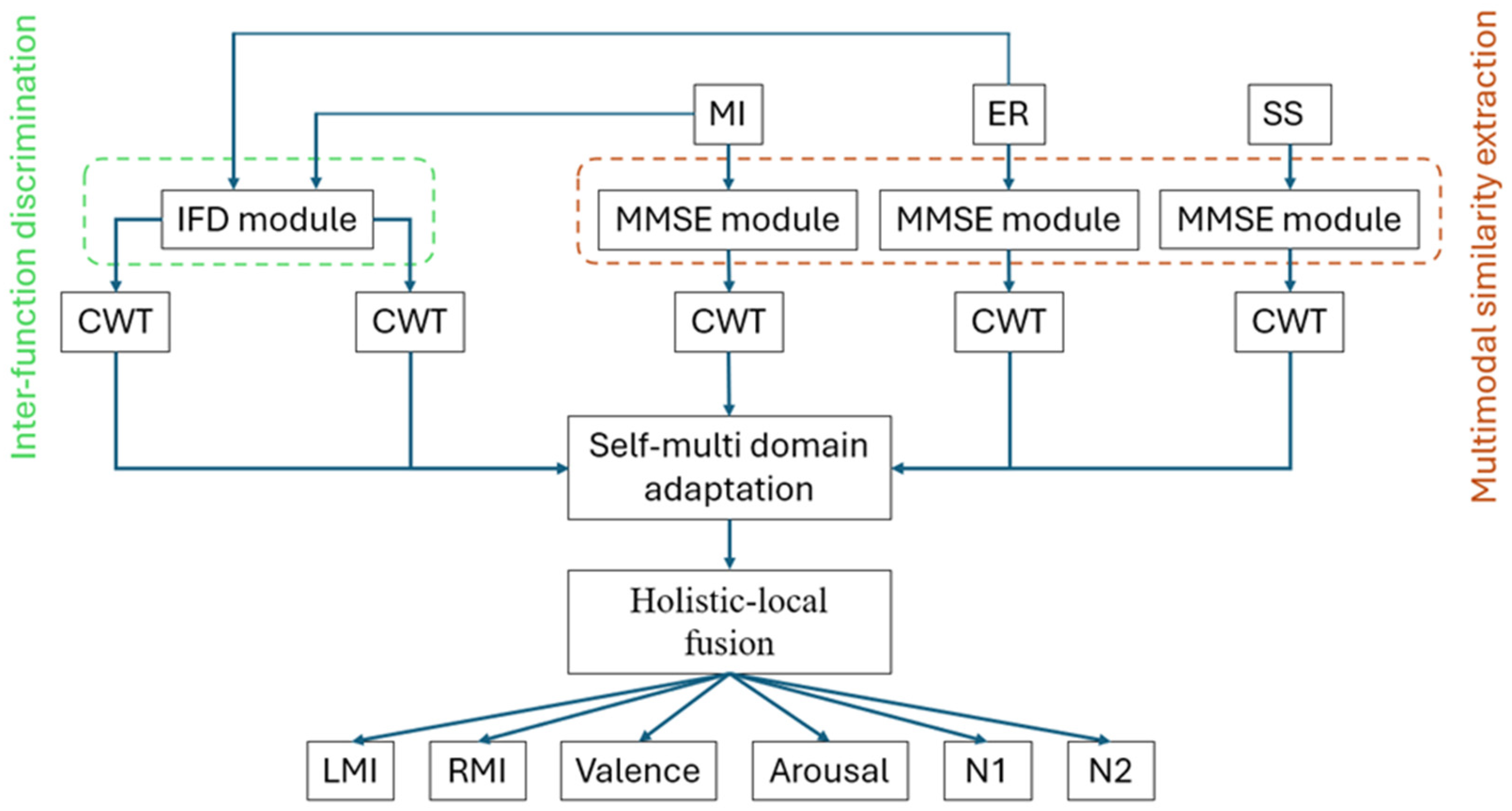
Figure 1. Overall proposed methodology.
Fractalfract 09 00585 g001
Figure 2. MMSE.
Figure 2. MMSE.
Fractalfract 09 00585 g002
Figure 3. SMDA.
Figure 3. SMDA.
Fractalfract 09 00585 g003
Figure 4. IFD.
Figure 4. IFD.
Fractalfract 09 00585 g004
Figure 5. HLF module.
Fractalfract 09 00585 g005
Figure 6. FDE of (a) LMI and (b) RMI.
Fractalfract 09 00585 g006
Figure 7. Student’s t-test. XSleepNet [35].
Fractalfract 09 00585 g007
Figure 8. Training and validation accuracy-loss graph.
Fractalfract 09 00585 g008
Table 1. Mean (MI/ER/SS) ablation accuracies in % for 1-shot and 10-shot learning using combined dataset. ✓: Indicates inclusion of the module.
ModulesMMSESMDAIFDHLFAccuracy
Data
1-shot 65.4/64.2/67.8
69.5/69.1/68.7
72.6/72.3/71.8
78.5/78.3/80.4
10-shot 70.3/69.6/73.2
75.1/73.6/77.4
78.2/76.8/82.4
84.5/81.7/89.3
Table 2. Mean accuracy (%) comparison of the proposed model with SOTAs for individual tasks. P (parameters’ count) in million, IT (inference time) in ms.
TasksAlgorithms1-Shot5-Shot10-Shot20-ShotPIT
MIMeta-L MI [15]67.473.174.3 *74.4 *97.4 *42.7 *
FSL-DA MI [16]67.1*75.874.4 *74.1 *196.6 *63 *
MI RelationNet [1]58.263.565.265.686.3 *42.7 *
IFSL-MI [13]56.260.364.4568.2--
SPD-CNN [17]-42.946.7-6.6 *26.5 *
EEG-CNN [56]44.051.555.259.617 *26 *
MI-SCNN [57]44.047.051.153.820.522.4 *
MI-HFDNN [58]55.359.763.466.4--
CFE-FSL MI [18]44.856.364.468.4--
Multi-BioSig-Net (proposed)69.563.774.875.927.8 *34.2 *
ERSVM [25]58.160.2 *63.7 *64.5 *26.3 *31 *
EEGNet [26]61.062.2 *64.5 *66.7 *11.8 *21.7 *
TPT [27]60.5-----
TCA [28]55.0-----
KPCA [29]56.8-----
MAML + ResNet-18 [24]70.0-----
Multi-BioSig-Net (proposed)66.769.473.775.127.8 *34.2 *
SSMetaSleepLearner [30]64.1 *67.2 *72.174.8 *5.2 *17.3 *
SleepEEGNet [31]71.5 *76.6 *84.384.5 *2.611.7 *
DeepSleepNet [32]70.2 *75.9 *82.085.6 *24.734 *
DeepSleepNet-Lite [33]72.4 *77.3 *84.085.1 *0.610.4 *
AttnSleep [34]75.6 *79.2 *84.486.8 *31.8 *45.2 *
XSleepNet [35]78.1 *80.6 *86.088.5 *5.616.7 *
Average Ensemble [36]--85.4-0.2 *11.8 *
SleepFCN [38]--84.8---
ResNetMHA [39]--84.3---
IITNet [40]--83.9---
TPON [41]--87.1---
Multi-BioSig-Net (proposed)81.683.487.388.227.8 *34.2 *
Entries with an asterisk (*) show reproduced accuracies.
Table 3. Mean accuracy (%) comparison of the proposed model with SOTAs for multi-task on the combined dataset of MI, ER, and ST. P (parameters’ count) in million, IT (inference time) in ms.
ModelTask1-Shot5-Shot10-Shot20-ShotPIT
Meta-L MI [15]MI53.261.465.768.697.4 *42.7 *
ER48.654.258.160.0
SS45.151.652.955.7
FSL-DA MI [16]MI61.768.371.673.5196.6 *63 *
ER55.358.760.163.8
SS51.553.757.159.4
MI RelationNet [1]MI52.056.359.861.686.3 *42.7 *
ER49.651.553.155.7
SS47.451.352.654.8
EEG-CNN [56]MI48.456.360.565.717 *26 *
ER48.255.960.365.2
SS47.855.459.764.8
MI-SCNN [57]MI43.344.646.549.620.522.4 *
ER40.742.443.645.1
SS40.241.643.044.6
SVM [25]MI55.759.461.362.326.3 *31 *
ER58.161.463.664.5
SS53.656.758.659.6
EEGNet [26]MI58.761.265.568.811.8 *21.7 *
ER60.063.567.872.6
SS56.860.362.665.3
MetaSleepLearner [30]MI57.361.664.868.15.2 *17.3 *
ER58.462.964.367.3
SS61.667.470.673.2
SleepEEGNet [31]MI69.471.674.376.72.611.7 *
ER66.768.170.273.8
SS73.778.481.682.5
DeepSleepNet [32]MI66.270.173.475.724.734 *
ER64.667.269.372.9
SS70.375.879.682.4
DeepSleepNet-Lite [33]MI68.572.874.676.10.610.4 *
ER67.370.173.575.2
SS72.778.481.383.6
AttnSleep [34]MI71.074.377.179.831.8 *45.2 *
ER70.472.876.578.3
SS73.679.182.484.2
XSleepNet [35]MI77.480.583.987.75.616.7 *
ER76.878.282.986.3
SS79.583.688.689.2
Average Ensemble [36]MI65.367.971.274.20.2 *11.8 *
ER61.665.870.872.3
SS70.576.781.783.6
Multi-BioSig-Net (proposed)MI78.582.784.587.927.8 *34.2 *
ER78.380.181.784.8
SS80.485.689.391.9
Asterisk (*) shows the reproduced values.
Table 4. FD, C and R2 values from Figure 6.
ResultLMI (Figure 6a)RMI (Figure 6b)
FD1.567771.01815
C0.997810.98444
R20.995620.96912
Disclaimer/Publisher’s Note: The statements, opinions and data contained in all publications are solely those of the individual author(s) and contributor(s) and not of MDPI and/or the editor(s). MDPI and/or the editor(s) disclaim responsibility for any injury to people or property resulting from any ideas, methods, instructions or products referred to in the content.