Abstract
We are especially interested in the general framework and ability of a semi-analytic method (SAM) to use the trigonometric basis function (TBF) in different domains. Moreover, the stabilizing effect of increasing boundary nodes on the convergence of the method when a level of noise is added to the boundary data of the inverse boundary value problem for the nonlinear Rayleigh–Stokes (R-S) equation is investigated. The solution of the ill-conditioned Rayleigh–Stokes equation which the equation is reduced to the linear system with corrupted boundary data by quasilinearization technical on nonlinear source terms relies on TBFs and radial basis functions (RBFs). Finally, the implementation of the scheme is supported by the numerical experiments.
1. Introduction
Systems of non-Newtonian fluids appear in a wide variety of applications, ranging from industry, machine learning, and food products to biology [1,2], galactic dynamics [3,4], and plasma physics [5,6,7,8]. There is significant literature studying the behavior of these fluids. In a more realistic scenario, the system encounters many models to overcome the difficulty of constructing fractional viscoelasticity in non-Newtonian fluids. The problems in this paper relate to a fractional model of inverse boundary value problem for the nonlinear R-S equation to describe the viscoelastic behavior of the flow as
where is a positive constant, denotes the Laplacian operator, is a given nonlinear source term and is the unknown boundary date, and the Riemann–Liouville fractional derivative of order ,( ) defined by [9]
Our work is motivated by constructing the mathematical model of parameter identification to establish equations where physical measurements are not available or contaminated by noises in the transport processes or fluid flows; consequently, we derive inverse problems in the system (1). These kinds of inverse problems have been extensively studied from theoretical and numerical points of view using regularized methods. The study of the convergence of a backward problem, which is ill-posed, has been proposed by the trigonometric method (TM) in nonparametric regression in [6]. Wei et al. show [10] that by applying the subordination principle, the semilinear R-S problem is not well-posed in mixed norm spaces as comapred to the results in spaces. The work in [11] also addresses the inverse problem for (1) with the inhomogeneous term, particularly investigating the regularity and ill-posedness of the solution. In addition, various regularization parameters have been proposed in [12,13], including prior and posterior regularization parameters, where a filter regularization method is proposed to determine the source term of the R-S equation. Ke et al. [14] take advantage of fixed-point arguments to develop schemes in which the solvability and Holder regularity of solutions are established.
During the last decades, meshless methods were shown to be very applicable across various fields, ranging from engineering [15,16,17] and mechanics [18,19] to economics [20,21,22]. Despite the considerable progress made in modeling and numerical approximation of the R-S equation, only some publications can be found on the inverse problem of the R-S equation by the meshless method [23,24,25]. By adopting a mesh-free method, the SAM based on the Grünwald difference approximation of the time derivative for solving the inverse heat problem is analyzed in [26]. Also, the convergence of the scheme is shown in [27], and an error estimate for the solution of the ill-conditioned time-fractional integro-differential equation is derived. As efficacious management of ill-posedness, the numerical analysis of the inverse problems is performed via the regularization strategy. Here, to reduce the difficulty of performing the regularization technique, a novel version of the SAM would apply to the inverse boundary value problem for the nonlinear R-S equation.
The TBF function in the scheme with parameters ℘ [28,29,30] is adopted to derive the particular solution with the inhomogeneous boundary condition. The basis exploited in the scheme provides more information on the approximate solution of boundary data with added random noise terms, enabling the scheme to get rid of the complexity of performing the regularization technique, be more flexible in choosing collocation nodes in comparing with Chebyshev polynomials [31,32], and more effective in handling the ill-conditioning matrices corresponding to the RBF [3,4].
The main difficulty lies in transforming the nonlinear term of the right-hand sides in Equation (1) into a linear term, which has been achieved through the linearization of this part in via quasilinearization techniques [33]. There is now a large body of work addressing the numerical approximation of fractional derivatives with applications. After discretizing the time variable, numerical strategy, and the quasilinearization technique coupled with the Crank–Nicolson technique to drive a system (Section 2). To derive the strong approximation of in the ill-conditioned R-S equation with the corrupted boundary data, we will restrict ourselves to the corrected basis TBF and RBF functions. In the end, the implementation of the scheme is supported by the numerical experiments in Section 3.
2. Derivation of SAM Scheme
Approximation of the fractional partial derivative operator appearing in Equation (1) requires the discretization of the time-dependent equation variable. To explain how we would derive such a discretization, let us divide into subintervals of length and denote , and introduce the following Riemann–Liouville integral of order by
In each interval , it is readily checked that
We have supposed that u is twice differentiable and the second derivative is continuous. Hence, by taking the integral of Equation (4), we obtain that u satisfies
in which there exists a constant which leads to [34]
It follows from Equation (1) that by integration on the following is obtained:
We assume that , , and are the approximation of , the linearization of , and the initial approximations of the , respectively. In this case we choose the initial values of the iteration . As a matter of fact, by using the quasilinearization technique, it is possible to introduce a small value . Such definition provides . Thus, it is readily checked thatthe approximation of the third and last terms in Equation (7) can be equivalently written as
In what follows, the Algorithm 1 illustrates the quasilinearization technique for the nonlinear R-S Equation (1).
| Algorithm 1: Quasilinearization technique |
| Enter the required simulation parameters such as , , ⋯, |
| Input: k, , , , ⋯, |
| Output: |
| function QuasiTec (, ) |
| Enter the initial condition |
| for : |
| Solve the system (9) by the SAM and find |
| if |
| Make an update for the left and the right-hand side of the system (9) |
| Do the process of the SAM with new initial value |
| else |
| end |
| end |
Using the approximation of Riemann–Liouville integral as in Equation (5) and the linearization structure of in Equation (8), also omitting small terms, we will rewrite the approximating Equation (7) as
which in turn approximate numerically by the SAM and , . The idea consists of choosing the operator , and the right-hand side of system (9) as
We will rewrite the system with boundary condition as
For the sake of efficiency, we would like to expand into the particular solution with the inhomogeneous and homogeneous boundary condition as and introduce TBF functions where for fixed ℘, we express them in the 2D-TBF [35,36,37]
and 3D-TBF as
For example, we can write the TBF description in the matrix form by
In order to have a unique approximation and guarantee the effectiveness of the scheme, we must choose ℘ a large enough such that in the 2D domain and in the 3D domain. The key basis function to express is the TBF, and we represent the approximate solution as
where are unknown coefficient. Since the approximate solution satisfies system (11), we have
We use and to denote corrected basis functions and Multiquadric RBF functions with shape parameter . Then the expansion of is divided into two parts as
Moreover, we know from the system (16) and the above expansion that the following system yields
The effectiveness of the correction function for this simulation scheme depends on the TBF expansions with the parameter ℘, as we have already remarked. By applying the TBF expansions, under the boundary condition (18), we have . To obtain the unknown coefficients and , we require that collocation nodes be used in simulation, and collocation nodes are employed for every time step to yield the following system
where we are added a random noise term into the accurate boundary conditions . Finally, due to the expansion of in Equation (17), which involves corrected basis functions and Multiquadric RBF functions, collocation nodes in system (18) are employed to yield the following system:
3. Numerical Implementation
We implemented the meshless strategy proposed in Section 2 for the inverse problem in Equation (1). We tested the resulting scheme extensively for , and the noisy data are generated using the following formula
is a pseudo-random number added into the accurate boundary conditions, and represents the level of noise. First, we illustrate the efficiency of our meshless approach for solving inverse problems on the square domain. Then in Example 3, we deal with the nonlinear irregular exterior problem on the star domain generated by criteria , (). The accuracy is measured by
where N denotes the number of test points, while and
in which and are errors corresponding to the step size of time variable and .
Example 1.

The goal of this example is to highlight the efficiency of the scheme in two spatial dimensions with the exact solution and the source term [34]
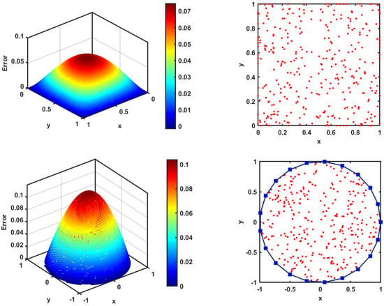
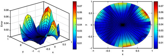
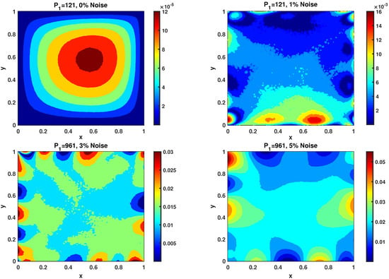
We verify our proposed scheme in Table 1 by comparing the maximum absolute error computed using the improved singular boundary method (ISBM) scheme and the SAM for various values of . Next, we apply these two numerical schemes to solve the problem on two domains and compare their computational errors. In Figure 1, Figure 2 and Figure 3, we report mesh errors of the numerical solutions with the ISBM and the SAM on square and circular domains without additive space noises. One can detect that the SAM on circular domain performs much better than the ISBM scheme, producing a much smaller . Now, we focus on the approximation with additive space noises. In Figure 3 the results of numerical experiments corresponding to various values of ν are presented. We start with the results for the parameters , . The total number of collocation points changes when a high level of noise is added to the boundary date to keep the accuracy.

Table 1.
Performance comparison of the SAM: , , , , for Example 1.

Figure 1.
The error mesh for the ISBM scheme in Example 1: , .

Figure 2.
The error mesh for the SAM in Example 1: , , , .

Figure 3.
The error contour for the SAM in Example 1 with the various values of at : , , , .
In order to further investigate the effect of the step time size and fractional order of derivative on the behavior of second-grade fluids, we will compute the as a function of based on the various values of at in Figure 4. Moreover, to see how the results are influenced by the collocation number point, we reported the errors for the selected level of noise in Figure 5. In the case of small-level noise at , the scheme provides more accurate results than when solving the problem with a noise level of using the same parameters. The following presents results for different values of the parameters and . We start with results for the parameter , , and , . Figure 6 shows the accuracy the problem versus various levels of added noise.
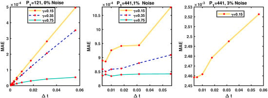
Figure 4.
Stability study for Example 1 with various values of at : , , , .
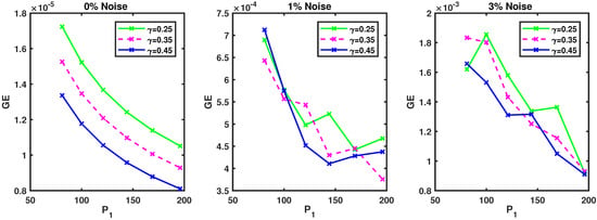
Figure 5.
Convergence study for Example 1 with various values of at : , , , .
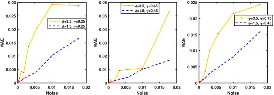
Figure 6.
Convergence study for Example 1 with various values of at : , , , , .
Example 2.
Consider Equation (1) with , and following condition
A solution of this problem was given analytically by Safari et al. [34] as follows:
Results of the simulation are tested extensively with the ISBM [34] scheme and the SAM on various and without added noise in Table 2. Next, mesh error results for the parameters , , when using the ISBM and the SAM are presented in Figure 7 and Figure 8. Compared to the problem with noise, the range of accuracy increases to , corresponding to , where the number of collocation point selection strategy works as intended. The total number of collocation points changes when a high level of noise is added to the boundary date to keep the accuracy.

Table 2.
Performance comparison between the SAM: , , , , , for Example 2.
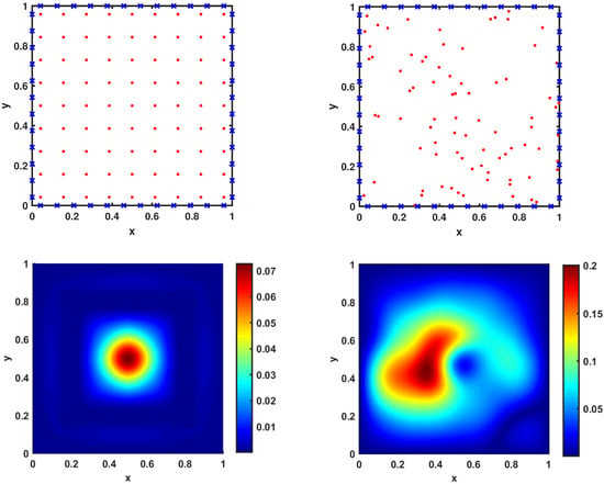
Figure 7.
The error mesh for the ISBM scheme in Example 1: , .
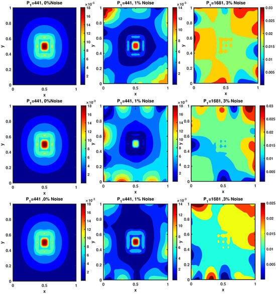
Figure 8.
The error contour for the SAM in Example 2 with the various values of at : (top to bottom) , , , .
Additionally, in Figure 9 we present the associated stability curves and the influence of the fractional order of derivative on the behavior of second-grade fluids and on the number of collocation points which is necessary for convergence of the scheme considering the parameters , , . Figure 10 shows the convergence simulations for various and ; here, one can see the convergence curves are slightly more affected by compared to the simulations for . Another effect of the level of added noise is that restrictions on the shape parameter, and the number of collocation points are necessary to ensure the convergence of the scheme. Although we have decreased the level of added noise to in Figure 11, the results are influenced more by the than in the previous simulations for .
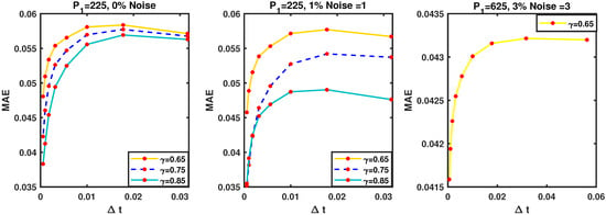
Figure 9.
Stability study for Example 2 with the various values of at : , .
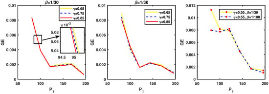
Figure 10.
Convergence study for Example 2 with the various values of at : , , , , .
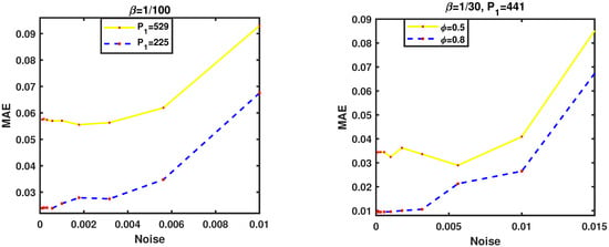
Figure 11.
Convergence study for Example 2 with the various values of at : , , , , .
Example 3.

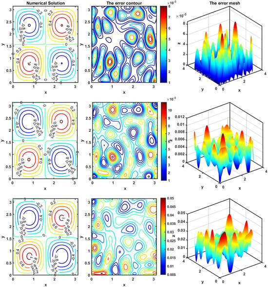
This example is intended to test the algorithm for the nonlinear irregular star-shape domain. Let us consider
where and the exact solution is [6]
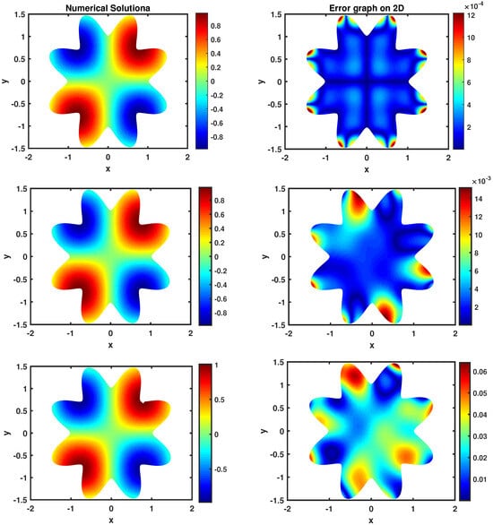
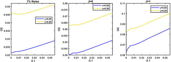
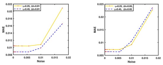
Here, we restrict our simulation results to one set of parameters, , , where the TM [6] scheme and the SAM on various γ with added noise are tested in Table 3. In the higher level of additive noise, failures of the SAM may also cause reduced accuracy, especially for small step sizes. In such a case we increase the total number of collocation points for a high level of noise added to the boundary date to keep the accuracy. We repeat the scheme on the star-shape and square-shape domains with a different additive noise. Figure 12 and Figure 13 compare the behavior of the scheme on the domains. Additionally, for each of these graphs, we provide the error mesh in 3D. Further, in Figure 14 we present the associated stability curves and the influence of the fractional order of derivative γ, with the color of noise defined by the value of the slope of the power spectrum density (PSD) of the linear regression on the log-log scale. The PSD of a noise scales as a power law of the frequency f, that is, , then the noise is white if and pink for [38].

Table 3.
Performance comparison of the SAM on : , , for Example 3.

Figure 12.
The error contour of Example 3 at : (top to down) , and Noise, , , , .

Figure 13.
The error contour of Example 3 at : (top to down) , and Noise, , , , .

Figure 14.
Stability study for Example 3 with white noise at : .
Example 4.
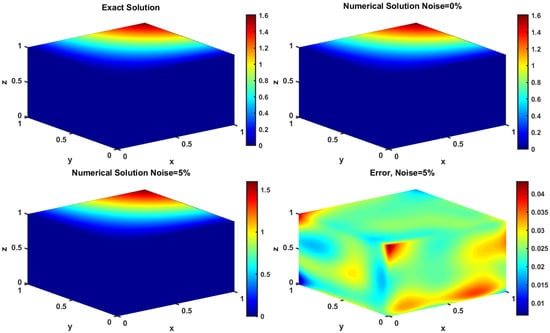
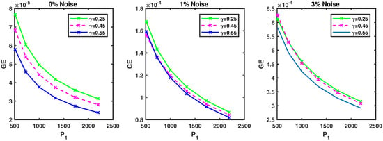
The goal of this example is to highlight the efficiency of the scheme in three spatial dimensions with the exact solution , and the associated source term. In order to investigate the approximation with additive space noises on the behavior of second-grade fluids, we illustrate the numerical solutions with the SAM on the domain. In Figure 15, the results of numerical experiments corresponding to various values of ν with the parameters , , and are presented. To see how much the results are influenced by the collocation number point, we illustrate the convergence simulations for various γ in Figure 16. Here, one can see the computational results converge as increases, and the use of optimal shape parameter provides considerably more accurate results. Figure 17 gives the accuracy of the problem versus various levels of added noise. Though we have decreased the level of added noise to , the results are more significantly influenced by the γ and . In addition, it can be observed that the computational results converge as ν approach to 0.

Figure 15.
The contours of the exact solution of Example 4 at : , , , .

Figure 16.
Convergence study for Example 4 with the various values of at : , , , , .

Figure 17.
Convergence study for Example 4 with the various values of at : , , , , .
4. Conclusions
The approach, which we have called the SAM, proposes to rigorously derive the boundary required solution corrupted by a level of added noises. Under general conditions without any compatibility condition on the problem data, the approach preserves the almost certain stability and convergence of the solutions for the selected level of noise. The scheme also has a linear rate of convergence for the nonlinear term of the R-S equation as the linearization of this part is performed by the quasilinearization technique. The proposed scheme is extensively tested in simulations with another numerical scheme with comparable stability properties.
Author Contributions
Methodology, F.S.; Software, F.S.; Validation, F.S. and X.F.; Investigation, F.S.; Writing—original draft, F.S.; Writing—review & editing, X.F.; Project administration, F.S. and X.F.; Funding acquisition, X.F. All authors have read and agreed to the published version of the manuscript.
Funding
The author thanks the editor and anonymous reviewers for their constructive comments on the manuscript. The work in this paper is supported the National Key Research and Development Program of China (2023YFB3711500).
Institutional Review Board Statement
Not applicable.
Data Availability Statement
The original contributions presented in this study are included in the article. Further inquiries can be directed to the corresponding author.
Conflicts of Interest
The authors declare no conflicts of interest.
Abbreviations
The following abbreviations are used in this manuscript:
| Nomenclature | |
| Co-ordinates | |
| t | Time |
| Nonlinear source term | |
| Unknown boundary date | |
| J | Number of TBfs |
| Number of boundary point | |
| Number of collocation point | |
| Boundary point | |
| Collocation point | |
| Level of noise | |
| N | Number of test nodes |
| Relative error | |
| CPU | Calculation time [s] |
| Greek symbols | |
| , m | Constants |
| Laplacian operator | |
| Order of fractional derivative | |
| Computational domain | |
| Boundary | |
| Gamma function | |
| Time step | |
| TBF functions | |
| ℘ | Scaling parameter |
| Corrected basis functions | |
| Multiquadric RBF functions | |
| Shape parameter | |
| Pseudo-random number |
References
- Shakib Arslan, M.; Abbas, Z.; Rafiq, M.Y. Biological flow of thermally intense cilia generated motion of non-Newtonian fluid in a curved channel. Adv. Mech. Eng. 2023, 15, 1–11. [Google Scholar] [CrossRef]
- Çolak, A.B. Analysis of the Effect of arrhenius activation energy and temperature dependent viscosity on non-newtonian maxwell nanofluid bio-convective flow with partial slip by artificial intelligence approach. Chem. Thermodyn. Therm. Anal. 2022, 6, 100039. [Google Scholar] [CrossRef]
- Ruggiero, M.L.; Ortolan, A.; Speake, C.C. Galactic dynamics in general relativity: The role of gravitomagnetism. Class. Quantum Gravity 2022, 39, 225015. [Google Scholar] [CrossRef]
- Scalera, G. A Non-Newtonian View of the Universe Derived from Hydrodynamic Gravitation and Expanding Earth. J. Mod. Phys. 2022, 13, 11. [Google Scholar] [CrossRef]
- Zhaosheng, Y.; Jianzhong, L. Numerical research on the coherent structure in the viscoelastic second-order mixing layers. Appl. Math. Mech. 1998, 19, 717–723. [Google Scholar] [CrossRef]
- Tuan, N.H.; Zhou, Y.; Thach, T.N.; Can, N.H. Initial inverse problem for the nonlinear fractional Rayleigh-Stokes equation with random discrete data. Commun. Nonlinear Sci. Numer. Simul. 2019, 78, 104873. [Google Scholar] [CrossRef]
- Liu, X.; Li, D. A link between a variable-order fractional Zener model and non-Newtonian time-varying viscosity for viscoelastic material: Relaxation time. Acta Mech. 2021, 232, 1–13. [Google Scholar] [CrossRef]
- Binhua, F.; Chen, R.; Liu, J. Blow-up criteria and instability of normalized standing waves for the fractional Schrödinger-Choquard equation. Adv. Nonlinear Anal. 2020, 10, 311–330. [Google Scholar] [CrossRef]
- Luc, N.H.; Lan, D.; O’Regan, D.; Tuan, N.A.; Zhou, Y. On the initial value problem for the nonlinear fractional Rayleigh-Stokes equation. J. Fixed Point Theory Appl. 2021, 23, 1–28. [Google Scholar] [CrossRef]
- He, J.W.; Zhou, Y.; Peng, L.; Ahmad, B. On well-posedness of semilinear Rayleigh-Stokes problem with fractional derivative on RN. Adv. Nonlinear Anal. 2021, 11, 580–597. [Google Scholar] [CrossRef]
- Tran Bao, N.; Nguyen Hoang, L.; Vo Van, A.; Nguyen, H.T.; Zhou, Y. Existence and regularity of inverse problem for the nonlinear fractional Rayleigh-Stokes equations. Math. Methods Appl. Sci. 2021, 44, 2532–2558. [Google Scholar] [CrossRef]
- Liu, S. Filter Regularization Method for Inverse Source Problem of the Rayleigh-Stokes Equation. Taiwan. J. Math. 2023, 1, 1–15. [Google Scholar] [CrossRef]
- Ashurov, R.; Mukhiddinova, O. Inverse problem of determining the order of the fractional derivative in the Rayleigh-Stokes equation. arXiv 2023, arXiv:2303.10669. [Google Scholar] [CrossRef]
- Ke, T.D.; Thang, N.N. On Global Solvability and Regularity for Generalized Rayleigh-Stokes Equations with History-Dependent Nonlinearities. Mediterr. J. Math. 2023, 20, 107. [Google Scholar] [CrossRef]
- Sriram, V.; Ma, Q.W. Review on the local weak form-based meshless method (MLPG): Developments and Applications in Ocean Engineering. Appl. Ocean Res. 2021, 116, 102883. [Google Scholar] [CrossRef]
- Wang, F.; Ahmad, I.; Ahmad, H.; Alsulami, M.D.; Alimgeer, K.S.; Cesarano, C.; Nofal, T.A. Meshless method based on RBFs for solving three-dimensional multi-term time fractional PDEs arising in engineering phenomenons. J. King Saud Univ. 2021, 33, 101604. [Google Scholar] [CrossRef]
- Srivastava, M.H.; Ahmad, H.; Ahmad, I.; Thounthong, P.; Khan, N.M. Numerical simulation of three-dimensional fractional-order convection-diffusion PDEs by a local meshless method. Therm. Sci. 2020, 25, 347–358. [Google Scholar] [CrossRef]
- Safari, F.; Chen, W. Coupling of the improved singular boundary method and dual reciprocity method for multi-term time-fractional mixed diffusion-wave equations. Comput. Math. Appl. 2019, 78, 1594–1607. [Google Scholar] [CrossRef]
- Fu, Z.; Xi, Q.; Gu, Y.; Li, J.; Qu, W.; Sun, L.; Wei, X.; Wang, F.; Lin, J.; Li, W. Singular boundary method: A review and computer implementation aspects. Eng. Anal. Bound. Elem. 2023, 147, 231–266. [Google Scholar] [CrossRef]
- Guerra, A.; Belinha, J.; Natal Jorge, R. A preliminary study of endothelial cell migration during angiogenesis using a meshless method approach. Int. J. Numer. Method. Biomed. Eng. 2020, 36, e3393. [Google Scholar] [CrossRef]
- Yu, S.; Sun, Z.; Yu, J.; Yang, J.; Zhu, C. An improved meshless method for modeling the mesoscale cracking processes of concrete containing random aggregates and initial defects. Constr. Build. Mater. 2023, 363, 129770. [Google Scholar] [CrossRef]
- Grabski, J.K.; Mrozek, A. Identification of elastoplastic properties of rods from torsion test using meshless methods and a metaheuristic. Comput. Math. Appl. 2021, 92, 149–158. [Google Scholar] [CrossRef]
- Salah, F.; Zainal, A.A.; Ching, D.L.C. New exact solution for Rayleigh-Stokes problem of Maxwell fluid in a porous medium and rotating frame. Results Phys. 2011, 1, 9–12. [Google Scholar] [CrossRef]
- Yu, B.; Jiang, X.; Qi, H. An inverse problem to estimate an unknown order of a Riemann-Liouville fractional derivative for a fractional Stokes’ first problem for a heated generalized second grade fluid. Acta Mech. Sin. 2015, 31, 153–161. [Google Scholar] [CrossRef]
- Ashurov, R.; Mukhiddinova, O.; Umarov, S. A Non-Local Problem for the Fractional-Order Rayleigh-Stokes Equation. Fractal Fract. 2023, 7, 490. [Google Scholar] [CrossRef]
- Safari, F. Solving multi-dimensional inverse heat problems via an accurate RBF-based meshless technique. Int. J. Heat Mass Transf. 2023, 209, 124100. [Google Scholar] [CrossRef]
- Safari, F. An accurate RBF-based meshless technique for the inverse multi-term time-fractional integro-differential equation. Eng. Anal. Bound. Elem. 2023, 153, 116–125. [Google Scholar] [CrossRef]
- Kuznetsov, D.F. A comparative analysis of efficiency of using the Legendre polynomials and trigonometric functions for the numerical solution of Ito stochastic differential equations. Comput. Math. Math. Phys. 2019, 59, 1236–1250. [Google Scholar] [CrossRef]
- Safari, F.; Jing, L.; Lu, J.; Chen, W. A meshless method to solve the variable-order fractional diffusion problems with fourth-order derivative term. Eng. Anal. Bound. Elem. 2022, 143, 677–686. [Google Scholar] [CrossRef]
- Amiri, S.; Hajipour, M.; Baleanu, D. A spectral collocation method with piecewise trigonometric basis functions for nonlinear Volterra-Fredholm integral equations. Appl. Math. Comput. 2020, 370, 124915. [Google Scholar] [CrossRef]
- Ghimire, B.K.; Li, X.; Chen, C.S.; Lamichhane, A.R. Hybrid Chebyshev polynomial scheme for solving elliptic partial differential equations. J. Comput. Appl. Math. 2020, 364, 112324. [Google Scholar] [CrossRef]
- Shivanian, E.; Keshtkar, M.; Navidi, H. Heat transfer from convecting-radiating fin through optimized Chebyshev polynomials with interior point algorithm. Nonlinear Eng. 2019, 9, 102–110. [Google Scholar] [CrossRef]
- Safari, F.; Tong, Q.; Tang, Z.; Lu, J. A Meshfree Approach for Solving Fractional Galilei Invariant Advection-Diffusion Equation through Weighted-Shifted Grünwald Operator. Mathematics 2022, 10, 4008. [Google Scholar] [CrossRef]
- Safari, F.; Sun, H. Improved singular boundary method and dual reciprocity method for fractional derivative Rayleigh-Stokes problem. Eng. Comput. 2020, 37, 3151–3166. [Google Scholar] [CrossRef]
- Zhang, Y.; Lin, J.; Reutskiy, S. A novel Gaussian-cubic-based backward substitution method using symmetric variable shape parameter. Eng. Anal. Bound. Elem. 2023, 155, 1069–1081. [Google Scholar] [CrossRef]
- Lin, J. Simulation of 2D and 3D inverse source problems of nonlinear time-fractional wave equation by the meshless homogenization function method. Eng. Comput. 2022, 38, 3599–3608. [Google Scholar] [CrossRef]
- Zhang, Y.; Rabczuk, T.; Lu, J.; Lin, S.; Lin, J. Space-time backward substitution method for nonlinear transient heat conduction problems in functionally graded materials. Comput. Math. Appl. 2022, 124, 98–110. [Google Scholar] [CrossRef]
- Bakalis, E.; Lugli, F.; Zerbetto, F. Daughter Coloured Noises: The Legacy of Their Mother White Noises Drawn From Different Probability Distributions. Fractal Fract. 2023, 7, 600. [Google Scholar] [CrossRef]
Disclaimer/Publisher’s Note: The statements, opinions and data contained in all publications are solely those of the individual author(s) and contributor(s) and not of MDPI and/or the editor(s). MDPI and/or the editor(s) disclaim responsibility for any injury to people or property resulting from any ideas, methods, instructions or products referred to in the content. |
© 2025 by the authors. Licensee MDPI, Basel, Switzerland. This article is an open access article distributed under the terms and conditions of the Creative Commons Attribution (CC BY) license (https://creativecommons.org/licenses/by/4.0/).