Article

Real-Time Efficiency Prediction in Nonlinear Fractional-Order Systems via Multimodal Fusion

School of Mechanical Engineering, Yanshan University, Qinhuangdao 066004, China
*
Author to whom correspondence should be addressed.
These authors contributed equally to this work.
Fractal Fract. 2025, 9(8), 545; https://doi.org/10.3390/fractalfract9080545
Submission received: 1 July 2025 / Revised: 7 August 2025 / Accepted: 17 August 2025 / Published: 19 August 2025
(This article belongs to the Special Issue Artificial Intelligence and Fractional Modelling for Energy Systems)

Abstract

Rod pump systems are complex nonlinear processes, and conventional efficiency prediction methods for such systems typically rely on high-order fractional partial differential equations, which severely constrain real-time inference. Motivated by the increasing availability of measured electrical power data, this paper introduces a series of prediction models for nonlinear fractional-order PDE systems efficiency based on multimodal feature fusion. First, three single-model predictions—Asymptotic Cross-Fusion, Adaptive-Weight Late-Fusion, and Two-Stage Progressive Feature Fusion—are presented; next, two ensemble approaches—one based on a Parallel-Cascaded Ensemble strategy and the other on Data Envelopment Analysis—are developed; finally, by balancing base-learner diversity with predictive accuracy, a multi-strategy ensemble prediction model is devised for online rod pump system efficiency estimation. Comprehensive experiments and ablation studies on data from 3938 oil wells demonstrate that the proposed methods deliver high predictive accuracy while meeting real-time performance requirements.

1. Introduction

With the sustained expansion of global energy demands, petroleum has established itself as a strategically vital energy resource that underpins the international economic framework. The beam pumping unit system [1], a predominant artificial lift technology for crude oil extraction, has been extensively deployed in stripper and marginal well operations due to its well-documented operational advantages. Characterized by mechanical robustness, operational reliability, and cost-effectiveness, this reciprocating pump system has become ubiquitous across major oilfield operations worldwide. However, prolonged oilfield depletion [2] has made the operational efficiency of beam pumping units an increasingly critical factor in production economics and energy optimization. As a result, the real-time efficiency monitoring and performance evaluation of beam pumping systems have emerged as key research priorities for improving oilfield production management and promoting sustainable energy utilization.
Traditional prediction models for estimating the efficiency of beam pumping systems include model-based approaches utilizing mathematical models and data-driven approaches based on historical data. Mathematical methods based on nonlinear fractional-order partial differential equations involve solving intricate nonlinear fractional-order partial differential equations. The mathematical formulation is presented as follows:
ρ A 2 u x , t t 2 = x E A u x , t x + E A τ α α t α u x , t x + f x , t
However, these traditional models, while offering valuable insights by combining geological and mechanical data, have three main drawbacks. They require large, detailed datasets and complex equations, struggle with the system’s nonlinear and time-varying behavior, and demand heavy computation, making real-time prediction and adaptive control impractical.
The data-driven soft sensing approaches for system efficiency estimation exhibit strong dependence on high-quality datasets while suffering from inherent limitations in physical interpretability, thereby significantly constraining parameter optimization and practical engineering applications. Furthermore, individual models demonstrate notable vulnerability to outliers, and conventional ensemble strategies are prone to either sensitivity issues or overfitting risks, ultimately compromising the real-time performance of efficiency prediction. The utilization of measured electrical power time-series data for system efficiency prediction enhances real-time monitoring capabilities while introducing new technical challenges. As a characteristic temporal data modality, the power sequences combine with existing system parameters to form a heterogeneous multimodal dataset. Consequently, developing effective multimodal feature fusion methodologies emerges as the critical pathway for achieving substantial improvements in prediction accuracy.
To address these challenges, we propose a series of prediction models for evaluating the system efficiency of beam pumping wells. First, three base learners are developed: an Incremental Cross-Fusion Model, an Adaptive-Weight Late Fusion model, and a Two-Stage Progressive Feature Fusion model. Next, two ensemble frameworks are constructed using these base learners: a Parallel-Series Cascade Ensemble and a Data Envelopment Analysis-based ensemble. Finally, we introduce a multi-strategy ensemble prediction model for beam pumping well efficiency that balances base-learner diversity with predictive accuracy. The contributions of this work are as follows:
(1)
First, we propose three base fusion-based prediction models for real-time efficiency prediction in nonlinear fractional-order partial differential systems: Asymptotic Cross-Fusion, Adaptive-Weight Late Fusion, and Two-Stage Feature Fusion.
(2)
Then, the development of two ensemble strategies integrating the base prediction models for real-time efficiency prediction in nonlinear fractional-order partial differential systems: a Parallel-Series Cascade strategy and a Data Envelopment Analysis strategy.
(3)
Finally, we introduce a multi-strategy ensemble prediction model for real-time efficiency prediction in nonlinear fractional-order partial differential equation systems.

2. Related Work

2.1. Mathematical Models

Prediction models for beam pumping system efficiency have predominantly relied on mathematical models grounded in the rod–string’s longitudinal vibration. Gibbs [3] first derived the fundamental rod–string vibration equation. Lekia [4] then introduced a rod–fluid coupled vibration simulation model. Xing [5,6] proposed a strongly nonlinear longitudinal vibration simulation model, while Moreno [7] formulated a nonlinear vibration equation for directional wells. Tarmigh [8] presented a two-phase flow-based vibration equation, and Yin [9] obtained an analytical solution for multi-tapered rod–string vibration. Wang [10] developed a simplified solid–thermal vibration model, and Qin [11] established an equivalent damping coefficient via friction energy-conservation principles. Ma [12] constructed a multiphase-flow simulation prediction model, whereas Langbauer [13] applied finite-element methods to derive the vibration equation. Lukasiewicz [14] addressed deviated wells, and W [15] proposed a gas–liquid separation-based model. Lekia [4] also formulated motion equations for surface equipment coupled with rod–fluid dynamics. Li [11] accounted for viscous and local damping losses, and Wang [16] introduced an axial–transverse coupled vibration simulation for deviated wells. Finally, Dong [17] examined the effects of real-time power-frequency variation and motor–load torque fluctuation on crank motion, rod–string vibration, and system power parameters. Although these traditional models integrate geological and mechanical data to yield valuable theoretical insights, they exhibit three primary limitations. First, they demand extensive, high-fidelity datasets and intricate mathematical formulations. Second, they lack robustness in capturing the intrinsic nonlinear dynamics and time-varying characteristics of the system. Third, their substantial computational overhead renders real-time prediction and adaptive control impractical and cost-prohibitive.

2.2. Prediction Models of System Efficiency Based on Historical Data

With the advancement of machine-learning technologies, an increasing number of studies have tackled the prediction of beam pumping system efficiency using data-driven approaches. Tan [18] employed time-series models, while Ma [19,20] investigated both graph-neural-network architectures and stacking-ensemble frameworks. However, these methods depend on large historical datasets and typically utilize either a single-model strategy or conventional ensemble techniques; consequently, they [21,22,23] often lack real-time responsiveness, exhibit reduced prediction accuracy, and suffer from limited robustness.

2.3. Multimodal Feature Fusion Networks

In recent years, advancements in sensor technologies have enabled the acquisition of multimodal data characterized by heterogeneous modalities. To address multimodal feature-fusion challenges, various methodologies have been proposed and successfully applied across domains. Zhou [24] developed an adversarial-learning-assisted perception importance fusion network. Chen [25] and Wang [26] introduced multimodal fusion techniques for sentiment analysis, while Milon and Zhao [27,28] proposed multimodal human-recognition systems. Moreover, multimodal fusion [29] has been exploited for fault diagnosis, fake information detection [30] using progressive fusion networks, depression detection [31], and human recognition [27]. Despite these advances, existing frameworks are tailored to specific problem domains and do not adequately capture the heterogeneous data types—including string-based, numerical, and sequential modalities—intrinsic to sucker rod pumping system efficiency prediction; consequently, current approaches remain insufficient for this application.

3. Basic Definitions

In this paper, “PCFE” denotes the Progressive Cross-Fusion Efficiency prediction model for rod pumping systems; “AWFE” denotes the Adaptive-Weight Late Fusion Efficiency prediction model; “TSPE” denotes the Two-Stage Progressive Feature-Fusion Efficiency prediction model; “EPCI” denotes the Parallel-Series Cascade Ensemble strategy model; “EDEA” denotes the Data Envelopment Analysis-based Online Efficiency prediction model; and “MEIE” denotes the Multi-strategy Ensemble Integration model for the online efficiency prediction of rod pumping systems. “QR” denotes quantile regression stratum.

4. Methodology

4.1. Prediction Models of Beam Pumping System Efficiency Based on Progressive Cross-Fertilization

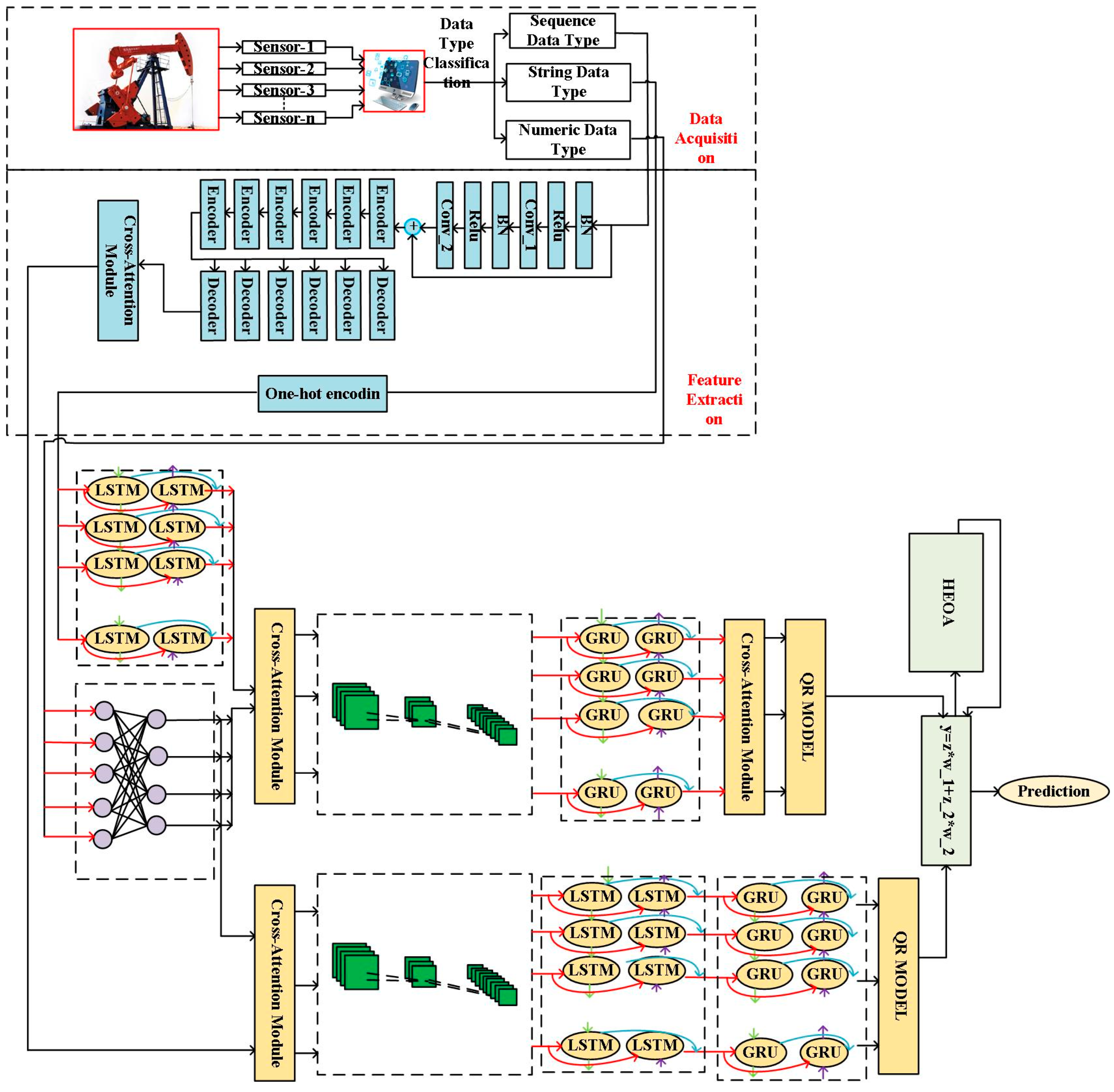
The factors influencing beam pumping system efficiency involve three types of data: string data, sequential data, and numerical data. Conventional feature processing methods often extract these features and concatenate them directly as the final feature set. This approach, however, frequently results in high dimensionality, information redundancy, and a failure to capture critical inter-feature relationships [32,33,34]. To overcome these limitations, we propose a prediction model for beam pumping system efficiency based on Progressive Cross-Fusion Efficiency (PCFE). The PCFE model comprises three modules: a feature extraction module, a feature fusion module, and a prediction module. The detailed structure and function of each module are described below, with the overall workflow illustrated in Figure 1 and Table 1.
In the feature extraction phase, we construct a multi-scale feature extraction framework through progressive integration of Residual Networks (ResNet), Transformer architecture, and Cross-Attention mechanisms. This integrated approach enables effective feature extraction for sequential data. For string-type data, feature extraction is performed using one-hot encoding. The mathematical formulation of the feature extraction process is defined as follows:
X = x 1 , x 2 , x 3 ,
Z = z 1 , z 2 , z 3 ,
F = R e s N e t X
T = T r a n s f o r m e r E n c o d e r F
X 1 = s o f t max T W h Q T W h K T d h T W h V h = 1 H W O
Z 1 = O n e h o t Z
where X is the raw sequence data; Z is the raw string data; X 1 is the extracted features from the sequence data; Z 1 is the extracted features from the string data; R e s N e t is a ResNet neural network; T r a n s f o r m e r E n c o d e r is the Transformer neural network; O n e h o t is the one-hot coding mechanism; W h and W O are weights; and Q , K , and V are query, key, and value, respectively.
To better capture the structural characteristics of raw data and mitigate cross-modal disparities, this study proposes a progressive cross-feature fusion approach to enhance model robustness. The methodology integrates three components: Bidirectional Long Short-Term Memory (BiLSTM), Bidirectional Gated Recurrent Unit (BiGRU), and Cross-Attention mechanisms. Initially, features extracted from string data Z 1 undergo processing through the BiLSTM network, mathematically formulated as follows:
Z 2 = L S T M Z 1 , t , h t 1 ; L S T M Z 1 , t , h t 1
where L S T M is a LSTM neural network.
Subsequently, the output Z 2 from the BiLSTM network and the extracted sequence features X 1 are passed to the Cross-Attention module to enable deep interaction between the two. The mathematical formulation of this process is provided in Equation (8).
Z 3 = X 1 W V S o f t max Z 2 W Q X 1 W K Τ d h
where W V , W Q , and W K are weights.
Finally, the output Z 3 of the Cross-Attention module is fed into the BiGRU network for further processing. The output of the BiGRU is then combined with numerical data via another Cross-Attention module to enable deep interaction, ultimately producing the fused features. The mathematical representation of this process is provided in Equations (10) and (11).
Z B i G R U = G R U Z 3 , t , h t 1 ; G R U Z 3 , t , h t 1
Z 4 = Z B i G R U W V S o f t max S W Q Z B i G R U W K Τ d h
where Z 2 , Z 3 is the intermediate variable for data fusion; Z 4 is the final fused features; S is to the numerical data features; G R U is a GRU neural network; and W V , W Q , and W K are weights.
During prediction, traditional single models often suffer from inaccurate predictions, vulnerability to disturbances, and a tendency to predict only conditional means—a limitation that may lead to local optima. To overcome this, we integrate CNN, BiGRU, an Attention mechanism, and a Quantile Regression (QR) layer, proposing a novel QRCNN–BiGRU–Attention model. The mathematical formulation of the model is presented below:
Z z = G R U C N N Z 4 , h t 1 ; G R U C N N Z 4 , h t 1
Z Attention = Z z S o f t max Z z Z z Τ d k
y = Q R Z Attention
where y is the final predicted value; C N N is a convolutional neural network; and Q R is the quantile regression stratum.

4.2. Adaptive Weight-Based Prediction Models of Efficiency of Late Fusion Pumping Well Systems

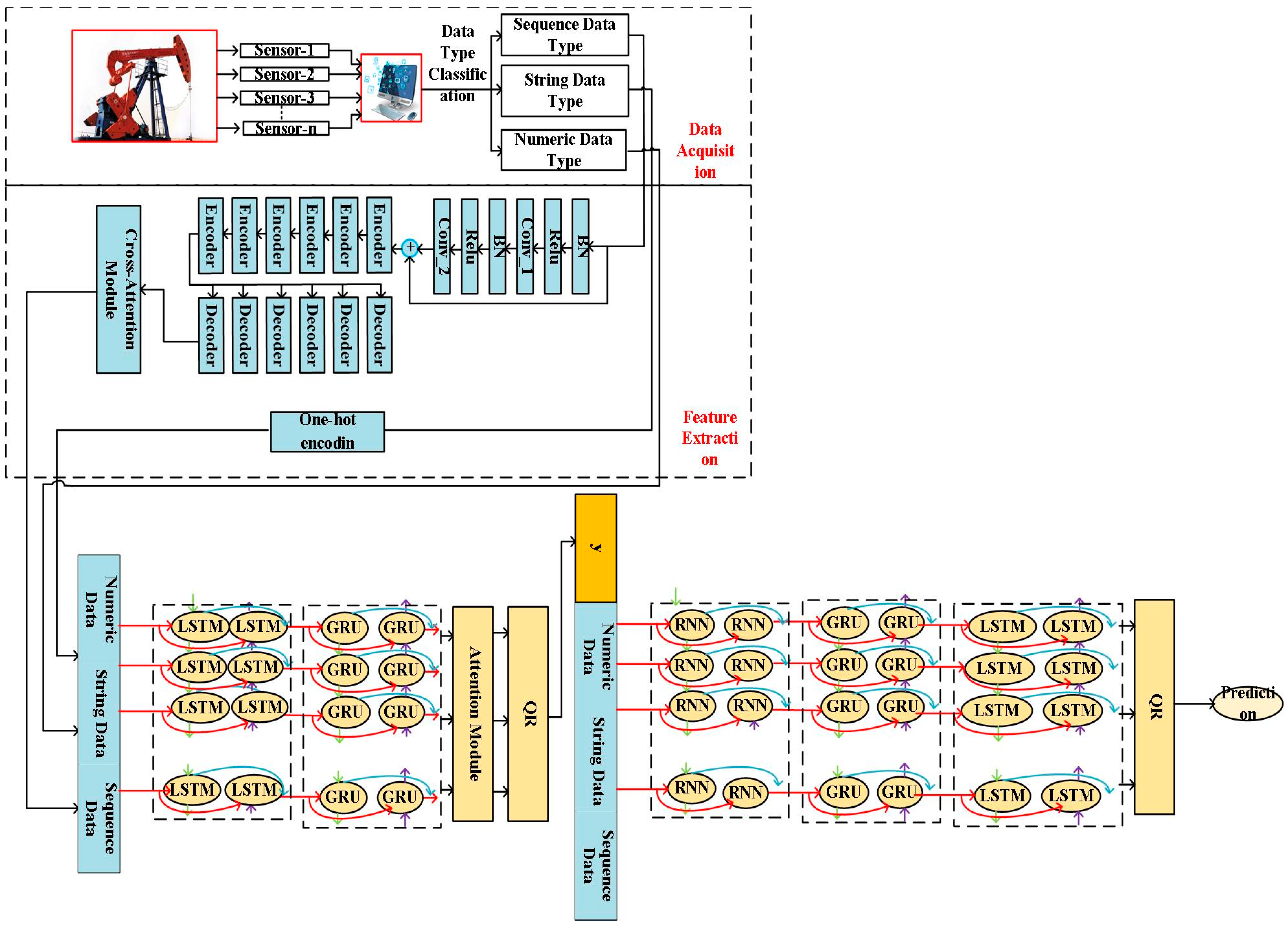
Today, widely used multi-modal feature fusion methods primarily include early fusion [32], intermediate fusion [33], and late fusion [34]. Late fusion strategies typically rely on summation, multiplication, and convolution operations. However, these approaches are often sensitive to scale and noise, struggle to handle heterogeneous features, and require additional parameter tuning. To address these limitations, we propose a prediction model method for beam pumping system efficiency based on a late fusion strategy inspired by human evolutionary algorithms. The proposed model consists of three main modules: a feature extraction module, an intermediate prediction module, and an Adaptive Weighting-based Feature Fusion module (AWFE). Each module is described in detail below, with the overall workflow illustrated in Figure 2 and Table 2.
In the feature extraction stage, we progressively integrate ResNet, Transformer, and Cross-Attention to construct a multi- scale feature extraction approach, enabling effective feature extraction for sequential data. For string data, feature extraction is performed using one-hot encoding. The mathematical model for the entire feature extraction process is described as follows:
X = x 1 , x 2 , x 3 ,
Z = z 1 , z 2 , z 3 ,
F = R e s N e t X
T = T r a n s f o r m e r E n c o d e r F
X 1 = s o f t max T W h Q T W h K T d h T W h V h = 1 H W O
Z 1 = O n e h o t Z
where X is the raw sequence data; Z is the raw string data; X 1 is the extracted features from the sequence data; Z 1 is the extracted features from the string data; R e s N e t is a ResNet neural network; T r a n s f o r m e r E n c o d e r is the Transformer neural network; O n e h o t is the one-hot coding mechanism; W h and W O are weight; and Q , K , and V are query, key, and value, respectively.
In the intermediate prediction module, inspired by the Boosting ensemble learning framework, we integrate CNN, BiGRU, Cross-Attention, BiLSTM, and quantile regression models in a cascaded manner. This leads to the proposal of two ensemble prediction models: the QRCNN–BiGRU–Cross-Attention model and the QRCNN-BiLSTM-BiGRU model. Initially, we use the Cross-Attention module to facilitate interaction between the numerical data and the extracted string features, as well as the extracted sequence features. The mathematical formulation of this process is presented below:
M 1 = L S T M Z t , h t 1 ; L S T M Z t , h t 1
M 2 = F N N S
M 3 = M 1 W V S o f t max M 2 W Q M 1 W K Τ d h
M 4 = X 1 W V S o f t max M 2 W Q X 1 W K Τ d h
where M 1 , M 2 , M 3 , M 4 is the intermediate variable generated after processing the data; F N N is a fully connected neural network; and W V , W Q , and W K are weights.
Subsequently, the fused intermediate variable is utilized as the input feature for the QRCNN–BiGRU–Cross-Attention ensemble prediction model to generate predictions. Similarly, the fused intermediate variable is also employed as the input feature for the QRCNN-BiLSTM-BiGRU ensemble prediction model. The mathematical formulations of these processes are presented below:
Z z 1 = G R U C N N M 3 , h t 1 ; G R U C N N M 3 , h t 1
Z c r o s s a t t e n t i o n 1 = Z z 1 W V S o f t max Z z 1 W Q Z z 1 W K Τ d h
y 11 = Q R Z c r o s s a t t e n t i o n 1
Z z 2 = L S T M C N N M 3 , h t 1 ; L S T M C N N M 3 , h t 1
Z z 3 = G R U C N N M 3 , h t 1 ; G R U C N N M 3 , h t 1
y 11 = Q R Z c r o s s a t t e n t i o n 1
y 12 = Q R Z z 3
where y 11 , y 12 is the intermediate prediction variable.
y = w 1 y 11 + w 2 y 12
w 1 = H E O A M S E
w 2 = H E O A M S E
where y is the final predicted value; w 1 , w 2 is the prediction weights; H E O A is to the human evolutionary algorithm; and W V , W Q , and W K are weights.

4.3. Prediction Models of Pumping Well System Efficiency Based on Two-Step Progressive Feature Fusion

Currently, widely used multi-modal feature fusion methods primarily include early fusion [32], intermediate fusion [33], and late fusion [34]. Early feature fusion often suffers from drawbacks such as the curse of dimensionality and noise propagation. Intermediate feature fusion typically faces high implementation complexity. Late fusion, on the other hand, often fails to capture deep-level interactions between modalities. To address these challenges, we propose a prediction model method for beam pumping system efficiency based on a Two-Stage Progressive Feature Fusion approach (TSPE). The model consists of three key phases: a feature extraction phase, a first-stage prediction model, and a second-stage prediction model. A detailed description of the model is provided below, with the workflow illustrated in Figure 3 and Table 3. In the feature extraction stage, we progressively integrate ResNet, Transformer, and Cross-Attention to construct a multi-scale feature extraction approach, enabling effective feature extraction for sequential data. For string data, feature extraction is performed using one-hot encoding. The mathematical model for the entire feature extraction process is described as follows:
X = x 1 , x 2 , x 3 ,
Z = z 1 , z 2 , z 3 ,
F = R e s N e t X
T = T r a n s f o r m e r E n c o d e r F
X 1 = s o f t max T W h Q T W h K T d h T W h V h = 1 H W O
Z 1 = O n e h o t Z
where X is the raw sequence data; Z is the raw string data; X 1 is the extracted features from the sequence data; Z 1 is the extracted features from the string data; R e s N e t is a ResNet neural network; T r a n s f o r m e r E n c o d e r is the Transformer neural network; O n e h o t is the one-hot coding mechanism; W h and W O are weight; Q , K , and V are query, key, and value, respectively.
In the first-stage prediction model phase, to address the limitations of single prediction models in terms of accuracy and robustness to disturbances, we propose an ensemble prediction model based on QRBiLSTM–BiGRU–Attention. Initially, the sequence data features X 1 , string data features Z 1 , and numerical data features S are concatenated. Subsequently, predictions are generated using the QRBiLSTM–BiGRU–Attention ensemble prediction model. The mathematical formulation of this process is presented below:
Z z 5 = L S T M X 1 , Z 1 , S , h t 1 ; L S T M X 1 , Z 1 , S , h t 1
Z z 6 = G R U Z z 5 , h t 1 ; G R U Z z 5 , h t 1
Z Attention - 2 = Z z 6 S o f t max Z z 6 Z z 6 Τ d k
y 13 = Q R Z Attention - 2
where y 13 is the intermediate prediction variable.
In the second-stage prediction model phase, to further enhance prediction accuracy and improve robustness to disturbances, we propose an ensemble prediction model based on QRBiRNN-BiGRU-BiLSTM. Initially, the intermediate prediction variables, sequence data features, string data features, and numerical data features are concatenated. Subsequently, predictions are generated using the QRBiRNN-BiGRU-BiLSTM ensemble prediction model. The mathematical formulation of this process is presented below:
Z z 7 = R N N X 1 , Z 1 , S , y 13 , h t 1 ; R N N X 1 , Z 1 , S , y 13 , h t 1
Z z 8 = G R U Z z 7 , h t 1 ; G R U Z z 7 , h t 1
Z Attention - 3 = Z z 8 S o f t max Z z 8 Z z 8 Τ d k
y 13 = Q R Z Attention - 3
where y is intermediate predictor variables and R N N is a RNN.

4.4. Prediction Models of Pumping Well System Efficiency Based on the Parallel-Strand Cascaded Integration Strategy

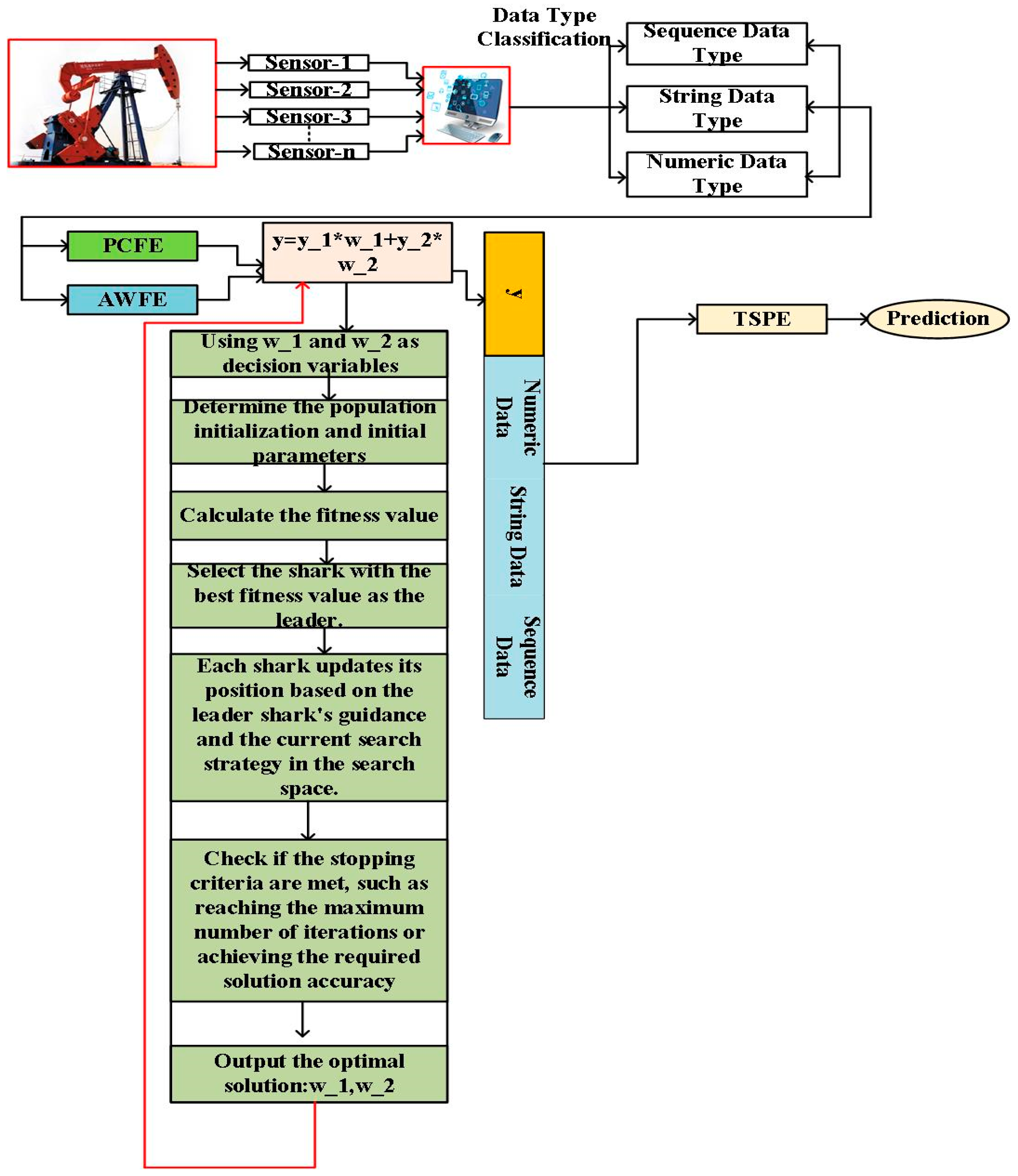
Ensemble learning is a machine learning approach that combines the predictions of multiple models to enhance overall performance. Common strategies include Bagging and Boosting. The Bagging strategy reduces variance, exhibits strong robustness, and is easily parallelizable, but its ability to improve bias is limited, making it suitable for high-variance models. In contrast, the Boosting strategy reduces bias and demonstrates strong predictive power, but it is slower to train, prone to overfitting, and sensitive to noise. To fully leverage the advantages of both Bagging and Boosting ensemble learning, we propose a prediction model method for beam pumping system efficiency based on a Parallel-Series Cascade Ensemble learning strategy (EPCI). The model primarily consists of two components: an initial Adaptive-Weight Parallel Ensemble prediction model and a subsequent Series Ensemble prediction model. A detailed description of the entire model is provided below, with the workflow illustrated in Figure 4 and Table 4.
During the initial modeling phase, we propose an adaptive parallel ensemble prediction framework. This architecture integrates PCFE and AWFE modules through an adaptively weighted late fusion mechanism. The weight coefficients are optimized via the Genghis Khan Shark Optimization (GKSO) algorithm to enhance prediction accuracy. The mathematical formulation of this integrated process is defined as follows:
y 6 = w 1 y P C F E + w 2 y A W F E
w 1 = G K S O M S E
w 2 = G K S O M S E
where G K S O is the Genghis Khan Shark Optimization algorithm and w 1 , w 2 is the optimization result of the Genghis Khan Shark Optimization algorithm.
In the later Series Ensemble prediction model phase, to fully leverage the advantages of various ensemble strategies, we innovatively integrate the two-stage Progressive Feature Fusion-based online prediction model for pumping well system efficiency with the initial Adaptive Parallel Ensemble prediction model in a serial manner. First, the prediction results from the initial Adaptive Parallel Ensemble prediction model are concatenated with the features extracted during the feature extraction phase.
X 5 = c o n n e c t i o n y 6 , X 1 , Z 1 , S
where c o n n e c t i o n is splicing.
Subsequently, the two-stage progressive feature fusion-based prediction model method for pumping well system efficiency is employed as the base learner for training, yielding more accurate prediction results. The mathematical formulation of this process is presented below:
y = T S P E X 5
where T S P E is the Two-Step Progressive Feature Fusion soft measure.

4.5. Online Prediction Models of Pumping Well System Efficiency Based on the Data Envelope Method Integration Strategy

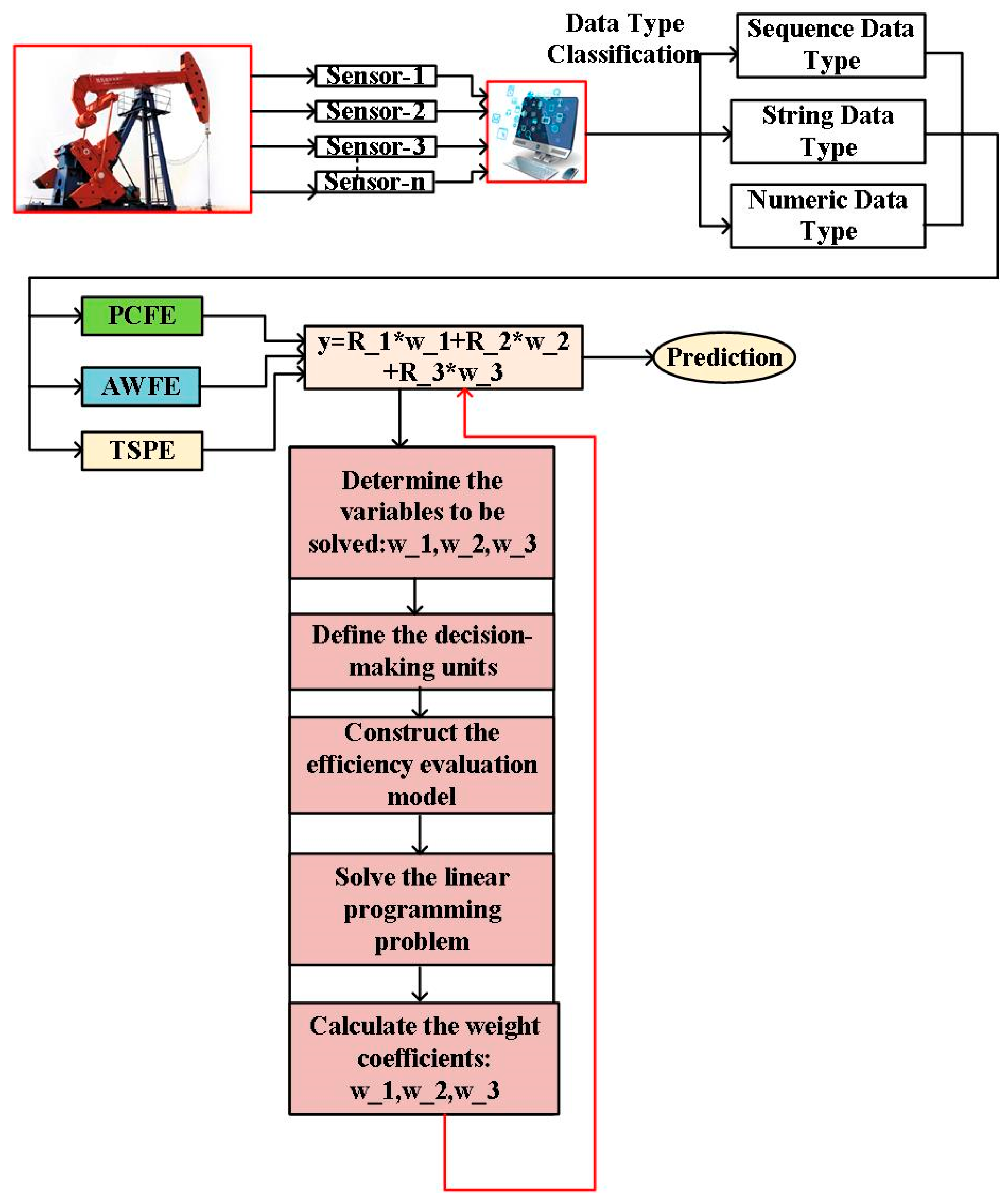
Today, most methods for combining base learners primarily include voting and averaging techniques. Simple ensemble methods such as voting and averaging offer certain advantages but also exhibit notable limitations, particularly in scenarios with low model diversity, significant performance disparities among base learners, or high levels of noise. These methods cannot often model relationships between base learners and cannot automatically adjust model weights, which restricts their potential for performance improvement. In contrast, the Data Envelopment Analysis (DEA) method can automatically compute data weights tailored to different decision-making units. Therefore, we introduce DEA and propose a prediction model method for beam pumping system efficiency based on a DEA ensemble strategy (EDEA). The prediction model consists of two phases: a base learner prediction phase and a DEA-based ensemble phase. A detailed description of the entire model is provided below, with the workflow illustrated in Figure 5 and Table 5.
First, the decision-making units are defined as: the Progressive Cross-Fusion method, the Adaptive-Weight Late Fusion method, and the Two-stage Progressive Feature Fusion Prediction Model method. The input vectors consist of factors influencing the system efficiency of pumping wells. The output vectors include the coefficient of determination for each base learner.
Next, a linear programming model is established. Here, we have three base learners, each with 28 inputs and 1 output. The primary objective of the DEA model is to maximize the efficiency of each base learner by solving the linear programming problem and determining the optimal weight coefficients. The mathematical formulation of the linear programming model is as follows:
For a decision cell k , its efficiency η k can be solved by the following linear programming:
M a x i m i z e : η k = λ 1 R 1 2 + λ 2 R 2 2 + λ 3 R 3 2 i = 1 29 θ i X i k
The constraints are as follows:
i = 1 3 λ i = 1 λ i 0 , i = 1 , 2 , 3 λ i 1 , i = 1 , 2 , 3 λ 1 R 1 2 + λ 2 R 2 2 + λ 3 R 3 2 1 M a x i m i z e : η k
where λ i is the weighting factor, which represents the contribution of the base learner in the integration; θ i is the efficiency value of the base learner with the goal of maximizing the efficiency; and η k is the efficiency of the first decision unit.
Finally, by solving the aforementioned linear programming problem, the efficiency θ of each base learner and the corresponding weight coefficients λ i can be obtained. These weight coefficients reflect the relative importance or contribution of each base learner within the ensemble. The final predicted value is derived by performing a weighted integration of the computed weight coefficients.
y = λ 1 y 11 + λ 2 y 12 + λ 3 y 13
where λ 1 , λ 2 , and λ 3 are the weights and y 11 , y 12 , and y 13 are the prediction result.

4.6. Online Prediction Models of Pumping Well System Efficiency Based on Integration of Multi-Integrated Strategies Integration

Currently, most studies focus on using single models as learners and employ specific ensemble strategies to integrate these base learners, aiming to explore the strengths and weaknesses of individual models. Alternatively, to improve ensemble accuracy, researchers have further investigated ensemble methods by incorporating accuracy and diversity analysis. However, these studies are typically based on single models, with limited exploration of integrating different ensemble strategies or balancing diversity and prediction accuracy in ensemble design. Therefore, by balancing the diversity and prediction accuracy among ensemble strategies, we propose a novel prediction model method for beam pumping system efficiency based on the integration of multiple ensemble strategies (MEIE). A detailed description of the entire model is provided below, with the workflow illustrated in Figure 6 and Table 6.
Step 1: Initially, the entire dataset was categorized by data type into string data, sequential data, and numerical data, and was then partitioned into training, validation, and test sets.
Step 2: Subsequently, the bootstrap resampling method was applied to the training set to randomly draw samples with replacement, yielding four distinct training subsets. Each subset was then used to evaluate both the EPCI soft sensing method and EDEA soft sensing method for rod pump system efficiency, resulting in eight base ensemble learners, as detailed below:
M = E P C I 1 , E D E A 1 , E P C I 2 , E D E A 2 , E P C I 3 , E D E A 3 , E P C I 4 , E D E A 4
Step 3: Next, to balance the diversity and prediction accuracy among the base ensemble strategy learners, we propose a novel method for selecting base ensemble strategy learners. This method incorporates diversity selection and accuracy selection analysis. In the diversity analysis module, an arbitrary model mod el i is selected from M to generate a validation set of prediction results y i . Another model mod el j is then selected to produce a validation set of prediction results y j . The Kendall rank correlation coefficient is calculated to determine the correlation coefficient z 1 between y i and y j . This process is repeated to compute the correlation coefficients z = z 1 , z 2 , z 3 , z 4 , z 5 , z 6 , z 7 among the predicted values of all models.
Step 4: The base models in a are reordered based on the magnitude of their correlation coefficients, forming M , a new set of base learner models, and M 2 , which exhibits a specific order. To ensure maximum diversity, the base ensemble strategy learner with the highest correlation after sorting is removed, resulting in a new set of base learner models, M 3 .
Step 5: The coefficients of determination of the remaining base ensemble strategy learners from Step 4 are arranged in descending order. To ensure the prediction accuracy of the ensemble, the smallest coefficient R 2 is discarded, leaving six base ensemble strategy learners. These learners form a new set of base learner models, M 4 .
Step 6: Finally, leveraging the Blending paradigm, the validation-set predictions of the remaining six base learners were aggregated to form a new training dataset for the meta-learner, which was then trained and subsequently evaluated on the final test set.

5. Experiment

5.1. Data Description

In our study, we randomly selected 3938 actual oil wells from a self-constructed database of a western Chinese oilfield. Due to the presence of unusable and missing data, we employed random sampling from the original dataset. When unusable data were encountered, they were discarded, and the sampling process was repeated until the required 3938 wells were obtained. The data types encompassed three categories: numerical, string, and sequential data. A sample of the dataset is presented in Table 7.
The analysis of Table 7 reveals that the dataset comprises a total of 29 features, including 28 influencing features and 1 predictive feature. The data types are categorized into three groups: “pumping unit model” and “Balancing method” are string types; “well inclination angle”, “dogleg severity”, and “electrical power curve” belong to the sequential data type; while the remaining features are numerical data types.

5.2. Data Pre-Processing and Evaluation Indicators

To comprehensively validate the rationality and predictive accuracy of the proposed model, the dataset was partitioned into training, validation, and test sets in a 0.7:0.15:0.15 ratio. Thereafter, to balance the impact of disparate feature units and scales on prediction performance, min–max normalization was applied to all input features. The formula for maximum–minimum normalization is shown below:
X = x x min x max x min
where x is the original data; x min is the minimum value in the dataset; and x max is the maximum value in the dataset.
To evaluate the validity and predictive accuracy of the proposed model, we use the quantile loss function and the coefficient of determination as evaluation metrics. Its calculation formula is given as follows:
L τ y i , y ^ i = τ y a c , j y p r , j i f   y a c , j y p r , j 1 τ y p r , j y a c , j i f   y a c , j < y p r , j
The mathematical model of the coefficient of determination is
R 2 = 1 i = 1 M y a c , j y p r , j 2 i = 1 M y a c , j ¯ y a c , j 2
where M is the total number of samples; y a c , j is the true value; and y p r , j is the predicted value.

5.3. Experimental Details

To validate the predictive accuracy of the proposed model, hyperparameters were tuned empirically via trial-and-error methods. The resulting parameter settings are as follows.
(1)
PCFE: To validate the accuracy of PCFE, the learning rate was 0.001, the number of training iterations was 500, the batch size was 256, and the optimizer was Adam. In the ResNet backbone, convolutional kernels measured 7 × 7 with a stride of 2 and padding of 3. The Transformer module comprised eight attention heads with an embedding dimension of eight. Both the BiLSTM and BiGRU subnets consisted of two hidden layers, each containing 25 units. In the QRCNN–BiGRU–Attention model, convolutional kernels measured 16 × 16 with a stride of 1 and no padding, the BiGRU component included two hidden layers of 12 units each, and the attention mechanism used four heads with an attention dimension of 24.
(2)
AWFE: To validate the accuracy of AWFE, the learning rate was 0.001, the number of training iterations was 100, the batch size was 128, and the optimizer was Adam. In the ResNet backbone, convolutional kernels measured 7 × 7 with a stride of 2 and padding of 3. The Transformer module comprised eight attention heads with an embedding dimension of eight. At the data-alignment layer, the BiLSTM consisted of one hidden layer of five units. In the QRCNN–BiGRU–Cross-Attention model, convolutional kernels measured 16 × 16 with a stride of 2 and padding of 1, the BiGRU featured one hidden layer of 12 units, and the Cross-Attention mechanism employed four attention heads with an embedding dimension of 24. In the QRCNN-BiLSTM-BiGRU variant, convolutional kernels measured 16 × 16 with a stride of 1 and automatic padding; the BiLSTM comprised one hidden layer of 12 units; and the Cross-Attention module again utilized four heads with an embedding dimension of 24. Finally, the human evolutionary algorithm was configured with a population size of 50 and 1000 iterations.
(3)
TSPE: To validate TSPE accuracy, the following hyperparameters were adopted, namely a learning rate of 0.001, 80 training iterations, and a batch size of 128, with Adam as the optimizer. The ResNet backbone utilized 7 × 7 convolutional kernels with stride 2 and padding 3. The Transformer module contained eight attention heads with an embedding dimension of 8. In the QRBiLSTM–BiGRU–Attention model, both BiLSTM and BiGRU subnetworks comprised two hidden layers of 20 units each. The QRBiRNN-BiGRU-BiLSTM variant featured single hidden layers of 64 units in each subnetwork (BiRNN, BiLSTM, and BiGRU).
(4)
EPCI: To validate EPCI accuracy, the multiple hyperparameters were adopted—the learning rate was 0.001; there were 1000 training iterations for PCFE, 100 for AWFE, and 376 for TSPE; and there was a uniform batch size of 128. All other parameters remained fixed.
(5)
EDEA: To validate EDEA accuracy, a learning rate of 0.001 was adopted. Training iterations were set to 500 for PCFE, 100 for AWFE, and 100 for TSPE, with a uniform batch size of 128. In the PCFE method, both BiLSTM and BiGRU modules contained two hidden layers of 32 units each. For the AWFE approach, the data-alignment layer’s BiLSTM module employed a single hidden layer with 10 units. All other hyperparameters remained constant.
(6)
MEIE: To validate the accuracy of the proposed multi-strategy ensemble prediction model method for rod pump system efficiency, the final ensemble model (QRBiLSTM–BiGRU–Attention) was configured with a learning rate of 0.001, a batch size of 64, and 500 training iterations. The BiLSTM component contained two hidden layers of 64 units each, while the BiGRU component featured one hidden layer with 64 units. All other hyperparameters remained unchanged.

5.4. Experimental Results and Analysis

To evaluate the accuracy of the proposed method, we conducted 10 experimental trials of six rod pump efficiency prediction models using the hyperparameters detailed in Section 5.3. Table 8 lists the mean and standard deviation of evaluation metrics for each model. The loss curves for training and validation sets, along with test-set prediction results, are shown in Figure 7.
As evidenced by Figure 7a and Table 8, the loss decreases rapidly during the initial 50 iterations. Beyond approximately 250 iterations, both training and validation loss curves asymptotically converge with near-complete overlap. The absence of validation loss rebound or further training loss reduction indicates minimal overfitting and confirms robust generalization capability. Data points align closely with the reference line (blue), while evaluation metrics (0.7961 and 1.8927) demonstrate PCFE’s consistent performance across varying target-value ranges.
From Figure 7b and Table 8, the loss decreases sharply within 10–20 iterations. Thereafter, both the training and validation loss curves level off, with the validation loss closely tracking the training loss and exhibiting no rebound or sustained increase, indicating that under the current hyperparameter configuration neither overfitting nor underfitting occurs. The scatter points align predominantly along the blue reference line, and the evaluation metrics are 0.7627 and 2.0835, demonstrating that the proposed AWFE maintains strong consistency across different target-value ranges.
As shown in Figure 7c and Table 8, the loss decreases sharply from approximately 8 to 3 within 0–20 iterations, followed by a brief plateau around iteration 10, and then continues to decline rapidly to about 2. Throughout the training, the validation loss closely tracks the training loss with minimal divergence, indicating that the proposed prediction model method exhibits neither significant overfitting nor underfitting. The scatter points are predominantly aligned along the blue reference line. Moreover, the evaluation metrics are 0.7693 and 2.0637, demonstrating that the proposed TSPE maintains strong consistency across different target-value ranges.
From Figure 7d and Table 8, it can be observed that within the first 20 iterations, the loss function decreased rapidly from approximately 8 to about 2.5, indicating that the proposed soft-sensing method quickly captured the principal trend during the initial training phase. After 200 iterations, the loss curves stabilized, with the training and validation losses closely overlapping and exhibiting no significant divergence, demonstrating the absence of severe overfitting or underfitting and confirming the model’s strong generalization capability. The scatter points are predominantly aligned along the blue reference line, and the evaluation metrics are 0.8685 and 1.5490, indicating that the proposed EPCI maintains good consistency across different target-value ranges.
From Figure 7e and Table 8, the blue scatter points closely follow the blue dashed reference line, indicating a high degree of agreement between the predicted and actual values. The overall coefficient of determination is 0.8581, and the loss metric is 1.7357. It is evident that prediction accuracy is highest in the medium-efficiency range, with a slight underestimation observed for a few extreme high-efficiency samples. Overall, the proposed EDEA demonstrates robust stability and accuracy across the entire efficiency spectrum.
From Figure 7f and Table 8, the scatter plot of the proposed method on the test set shows that most points are tightly distributed around the blue dashed reference line, indicating strong linear fitting performance across the full efficiency range. The overall coefficient of determination is 0.9335 and the loss metric is 1.2293. Predictions in the low-efficiency region exhibit no significant bias, while those in the medium-to-high-efficiency range show slight underestimation, and errors increase marginally for extreme high-efficiency samples. Overall, the model delivers accurate and stable predictions within the normal operating range.

6. Ablation Study

6.1. Ablation Study of the PCFE Prediction Models

To comprehensively evaluate the contribution of each component within the PCFE pre-prediction model framework to system efficiency prediction performance, ten ablation experiments were conducted for each element, and the mean and standard deviation of the evaluation metrics were computed. In the feature extraction branch ResNet–Transformer–Cross-Attention, we sequentially removed the Cross-Attention and Transformer modules. In the prediction branch QRCNN–BiGRU–Attention, we individually ablated the BiGRU and Attention components. Each ablation variant was then compared against the complete proposed method. Table 9 summarizes the evaluation metrics for all variants, and Table 10 describes the percent change for each ablation experiment.
As shown in Table 9 and Table 10, in the feature extraction branch, the removal of the Cross-Attention module reduces R2 from 0.7961 to 0.7746, a reduction of 2.71%, and raises L τ from 1.8927 to 1.9464, an increase of 2.83%. Further ablating the Transformer module decreases R2 from 0.7746 to 0.7564, a reduction of 2.35%, and increases L τ from 1.9464 to 2.0369, an increase of 4.65%. In the prediction branch, excluding the Attention component lowers R2 from 0.7961 to 0.7734, a reduction of 2.85%, and raises L τ from 1.8927 to 1.9564, an increase of 3.37%. Additionally, removing BiGRU reduces R2 from 0.7734 to 0.7552, a reduction of 1.82%, and increases L τ from 2.0264 to 2.0388, an increase of 4.21%. These results demonstrate that each key module—Cross-Attention, Transformer, Attention, and BiGRU—provides statistically significant improvements in feature extraction capability and predictive accuracy.

6.2. Ablation Study of the AWFE Prediction Models

To comprehensively assess the contribution of each component in the AWFE prediction framework to system efficiency forecasting, we conducted ten ablation experiments per component and computed the mean and standard deviation of the evaluation metrics. For the feature extraction module ResNet–Transformer–Cross-Attention, we removed the Cross-Attention component. In the prediction module QRCNN–BiGRU–Cross-Attention-1, we ablated the BiGRU, Cross-Attention, and CNN components separately. Similarly, for the prediction module QRCNN-BiLSTM-BiGRU-2, we sequentially removed the BiLSTM and BiGRU components. All ablated versions were systematically compared with the complete framework. The quantitative evaluation metrics of these variants are presented in Table 11. Table 12 describes the percent change for each ablation experiment.
In the feature extraction branch, ablating the Cross-Attention module reduces the R2 value from 0.7923 to 0.7756, a reduction of 2.11%, and increases the L τ from 1.8645 to 1.9900, an increase of 6.73%. In prediction branch 1, removing the Cross-Attention alone decreases the R2 from 0.7923 to 0.7714, a reduction of 2.64%, and increases the L τ from 1.8645 to 1.9904, an increase of 6.75%. Further ablating the BiGRU component reduces the R2 from 0.7714 to 0.7523, a reduction of 2.47%, and increases the L τ from 1.9904 to 2.1569, an increase of 8.37%. When the CNN component is also removed, the R2 decreases from 0.7714 to 0.7544, a reduction of 2.20%, and the L τ increases from 1.9904 to 2.1369, an increase of 7.36%. In prediction branch 2, ablating BiGRU reduces the R2 from 0.7923 to 0.7743, a reduction of 2.27%, and increases the L τ from 1.8645 to 1.9901, an increase of 6.74%. Subsequently removing the CNN component further decreases the R2 from 0.7923 to 0.7708, a reduction of 2.72%, and increases the L τ from 1.8645 to 2.0835, an increase of 11.74%. Finally, ablating the BiLSTM component decreases the R2 from 0.7708 to 0.7633, a reduction of 0.97%, and increases the L τ from 2.0835 to 2.1046, an increase of 1.01%. Collectively, these quantitative results indicate that each key component—Cross-Attention, BiGRU, CNN, and BiLSTM—provides statistically significant improvements in both feature extraction capability and prediction accuracy within the AWFE soft-sensor framework.

6.3. Ablation Study of the TSPE Prediction Models

To comprehensively assess the impact of each component in the TSPE prediction model on system efficiency forecasting, we conducted ten ablation experiments per component and reported the mean and standard deviation of the evaluation metrics. For the feature extraction branch ResNet–Transformer–Cross-Attention, the Transformer and Cross-Attention modules were removed. In the prediction branch QRBiLSTM–BiGRU–Attention, both the BiGRU layer and Attention mechanism were eliminated. Similarly, for the alternative prediction branch QRBiRNN-BiGRU-BiLSTM, the BiGRU and BiLSTM components were excluded. These ablated configurations were rigorously compared with the complete proposed method. Quantitative evaluation metrics for each ablation variant are summarized in Table 13. Table 14 describes the percent change for each ablation experiment.
In the feature extraction branch, ablating the Cross-Attention module produces an 8.00% relative decrease in R2 and a 24.4% relative increase in L τ . The subsequent removal of the Transformer module results in a further 2.71% reduction in R2 and a 13.01% increase in L τ . In prediction branch 1, omitting the Attention component causes a 6.50% drop in R2 and a 16.96% rise in L τ . The sequential removal of the BiGRU and BiLSTM layers leads to additional relative decreases in R2 of 1.45% and 1.42%, while the L τ increases by 9.38% and 8.02%, respectively. In prediction branch 2, successive ablations of the BiGRU, BiLSTM, and BiRNN modules result in relative reductions in R2 of 6.45%, 7.74%, and 7.82%, respectively, accompanied by increases in L τ of 16.11%, 21.91%, and 27.85%. The further removal of each BiGRU, BiRNN, and BiLSTM component contributes additional R2 declines of 2.50%, 3.89%, and 2.61%, along with L τ increases of 10.57%, 14.70%, and 5.63%, respectively. These quantitative results confirm that each key module—Cross-Attention, Transformer, BiGRU, BiLSTM, and their combinations—contributes significantly to enhanced feature extraction capability and improved prediction accuracy.

6.4. Ablation Study of the EPCI Prediction Models

To assess the contributions of PCFE, AWFE, and TSPE to system efficiency forecasting within the Parallel-Series Cascade Ensemble framework, we conducted ten ablation experiments per variant and calculated the means and standard deviations of the evaluation metrics. Table 15 summarizes the evaluation metrics for all ablation scenarios. Table 16 describes the percent change for each ablation experiment.
In the EPCI framework, removing both the AWFE and TSPE modules produces a 10.17% decrease in R2 and a 23.03% increase in L τ . Similarly, ablating both the PCFE and TSPE modules yields a 9.63% drop in R2 and a 26.59% rise in L τ , while eliminating both the PCFE and AWFE modules results in a 15.72% reduction in R2 and a 42.63% increase in L τ . These findings demonstrate that each key component—AWFE, TSPE, and PCFE—significantly enhances feature extraction and improves prediction accuracy.

6.5. Ablation Study of the EDEA Prediction Models

To comprehensively assess the EDEA framework’s pre-prediction performance, ten ablation studies were conducted on the PCFE, AWFE, and TSPE modules, and the mean and standard deviation of the evaluation metrics were calculated. Table 17 summarizes the evaluation metrics for each ablation variant. Table 18 describes the percent change for each ablation experiment.
In the EDEA framework, ablating the AWFE and TSPE modules results in a relative R2 decrease of 10.69% and a corresponding L τ increase of 12.85%. Similarly, removing the PCFE and TSPE modules causes an R2 drop of 8.52% and an L τ rise of 11.70%, while eliminating the PCFE and AWFE modules produces an R2 reduction of 11.83% accompanied by a 23.87% increase in L τ . These quantitative findings confirm that each key component—AWFE, TSPE, and PCFE—makes a statistically significant contribution to enhancing feature extraction capability and improving prediction accuracy.

6.6. Ablation Study of the MEIE Prediction Models

To comprehensively assess each component’s contribution within the MEIE framework to system efficiency forecasting, ten ablation experiments were performed on the EPCI and EDEA variants, and the mean and standard deviation of the evaluation metrics were calculated. Table 19 summarizes the evaluation metrics for each ablation experiment. Table 20 describes the percent change for each ablation experiment.
From Table 20, In the MEIE framework, removing the EPCI and EDEA modules leads to relative R 2 decreases of 5.71% and 6.01%, respectively, and corresponding L τ increases of 21.07% and 33.50%. These quantitative findings indicate that each key component makes a statistically significant contribution to enhancing feature extraction capability and improving prediction accuracy.

7. Conclusions

This study addresses the challenges of nonlinear dynamic characteristics and multi-source data fusion in predicting pumping well system efficiency by proposing an online prediction framework based on multi-strategy integration. By constructing three foundational prediction models—Progressive Cross-Fusion, Adaptive-Weight Late Fusion, and Two-Stage Progressive Feature Fusion—and combining them with Parallel-Series Cascade Ensemble strategies and Data Envelopment Analysis (DEA)-based ensemble strategies, the framework successfully enhances the accuracy and real-time performance of pumping well system efficiency prediction. Furthermore, to balance the diversity and prediction accuracy of base ensemble learners, a multi-ensemble strategy-based prediction model was proposed. Although the proposed models demonstrate strong performance in experiments, there remains room for improvement in handling extreme data and real-time deployment. Future research may focus on optimizing computational efficiency, further improving noise robustness, exploring additional ensemble strategy combinations to enhance adaptability and stability in real-world applications, and developing methods for the secure and reliable front-end deployment of the model in rod pumping systems.

Author Contributions

Both authors contributed equally to this work. All authors have read and agreed to the published version of the manuscript.

Funding

This work was supported by the National Natural Science Foundation of China under Grant 51974276.

Data Availability Statement

The datasets utilized in this study were obtained from a third-party industrial partner under strict confidentiality agreements. Due to commercial sensitivity and contractual restrictions, the raw data cannot be made publicly available. However, aggregated data, processed results, or specific subsets necessary to replicate critical findings may be provided upon reasonable request, subject to approval by the data owner and compliance with confidentiality protocols. Researchers interested in accessing limited data for verification purposes may contact the corresponding author to initiate a formal data-sharing request process.

Conflicts of Interest

The authors declare no conflicts of interest.

References

  1. Luan, G.-H.; He, S.-L.; Yang, Z.; Yang, Z.; Zhao, H.-Y.; Hu, J.-H.; Xie, Q.; Shen, Y.-H. A prediction model for a new deep-rod pumping system. J. Pet. Sci. Eng. 2011, 80, 75–80. [Google Scholar] [CrossRef]
  2. Lv, X.X.; Wang, H.X.; Zhang, X.; Liu, Y.X.; Chen, S.S. An equivalent vibration model for optimization design of carbon/glass hybrid fiber sucker rod pumping system. J. Pet. Sci. Eng. 2021, 207, 109148. [Google Scholar] [CrossRef]
  3. Gibbs, S.G. Predicting the behavior of sucker rod pumping systems. J. Pet. Technol. 1965, 61, 769–778. [Google Scholar] [CrossRef]
  4. Lekia, S.D.L.; Evans, R.D. A coupled rod and fluid Dynamic model for predicting the behavior of sucker-rod pumping system. SPE 1965, 21664, 30–45. [Google Scholar]
  5. Xing, M.; Zhou, L.; Zhang, C.; Xue, K.; Zhang, Z. Simulation Analysis of Nonlinear Friction of Rod String in Sucker Rod Pumping System. J. Comput. Nonlinear Dyn. 2015, 14, 091008. [Google Scholar] [CrossRef]
  6. Xing, M. Response analysis of longitudinal vibration of sucker rod string considering rod buckling. Adv. Eng. Softw. 2019, 99, 49–58. [Google Scholar] [CrossRef]
  7. Moreno, G.A.; Garriz, A.E. Sucker rod string dynamics in deviated wells. J. Pet. Sci. Eng. 2020, 184, 106534. [Google Scholar] [CrossRef]
  8. Tarmigh, M.; Behbahani-Nejad, M.; Hajidavalloo, E. Two-way fluid-structure interaction for longitudinal vibration of a loaded elastic rod within a multiphase fluid flow. J. Braz. Soc. Mech. Sci. Eng. 2023, 45, 572. [Google Scholar] [CrossRef]
  9. Jiaojian, Y.I.; Dong, S.U.; Yousheng, Y.A.G. Predicting multi-tapered sucker-rod pumping systems with the analytical solution. J. Pet. Sci. Eng. 2021, 197, 108115. [Google Scholar]
  10. Wang, X.; Lv, L.; Li, S.; Pu, H.; Liu, Y.; Bian, B.; Li, D. Longitudinal vibration analysis of sucker rod based on a simplified thermo-solid model. J. Comput. Nonlinear Dyn. 2021, 196, 107951. [Google Scholar] [CrossRef]
  11. Li, Q.; Chen, B.; Huang, Z.; Tang, H.; Li, G.; He, L.; Sáez, A. Study on Equivalent Viscous Damping Coefficient of Sucker Rod Based on the Principle of Equal Friction Loss. Math. Probl. Eng. 2019, 2019, 9272751. [Google Scholar] [CrossRef]
  12. Ma, B.; Dong, S. Coupling Simulation of Longitudinal Vibration of Rod String and Multi-Phase Pipe Flow in Wellbore and Research on Downhole Energy Efficiency. Energies 2023, 16, 4988. [Google Scholar] [CrossRef]
  13. Langbauer, C.; Antretter, T. Finite Element Based Optimization and Improvement of the Sucker Rod Pumping System. In Proceedings of the Abu Dhabi International Petroleum Exhibition & Conference, Abu Dhabi, United Arab Emirates, 3–6 November 2017. [Google Scholar]
  14. Lukasiewicz, S.A. Dynamic Behavior of the Sucker Rod String in the Inclined Well. In Proceedings of the SPE Production Operations Symposium, Oklahoma City, OK, USA, 7–9 April 1991. [Google Scholar]
  15. Hongbo, W.; Shimin, D.; Yang, Z.; Shuqiang, W.; Xiurong, S. Coupling simulation of the pressure in pump and the longitudinal vibration of sucker rod string based on gas-liquid separation. Shiyou Xuebao/Acta Pet. Sin. 2023, 44, 394–404. [Google Scholar]
  16. Wang, H.; Dong, S. Research on the Coupled Axial-Transverse Nonlinear Vibration of Sucker Rod String in Deviated Wells. J. Vib. Eng. Technol. 2021, 9, 115–129. [Google Scholar] [CrossRef]
  17. Dong, S.; Li, W.; Houtian, B.; Wang, H.; Chen, J.; Liu, M. Optimizing the running parameters of a variable frequency beam pumping system and simulating its dynamic behaviors. Jixie Gongcheng Xuebao/J. Mech. Eng. 2016, 52, 63–70. [Google Scholar] [CrossRef]
  18. Tan, C.; Deng, H.; Feng, Z.; Li, B.; Peng, Z.; Feng, G. Data-driven system efficiency prediction and production parameter optimization for PW-LHM. J. Pet. Sci. Eng. 2022, 209, 109810. [Google Scholar] [CrossRef]
  19. Ma, B.; Dong, S. A novel hybrid efficiency prediction model for pumping well system based on MDS-SSA-GNN. Energy Sci. Eng. 2024, 12, 3272–3288. [Google Scholar] [CrossRef]
  20. Ma, B.; Dong, S. A Hybrid Prediction Model for Pumping Well System Efficiency Based on Stacking Integration Strategy. Int. J. Energy Res. 2024, 2024, 8868949. [Google Scholar] [CrossRef]
  21. Wang, X.; Kihara, D.; Luo, J.; Qi, G.-J. ENAET: Self-trained ensemble autoencoding transformations for semi-supervised learning. arXiv 2019, arXiv:1911:09265. [Google Scholar]
  22. Ju, C.; Bibaut, A.; van der Laan, M. The relative performance of ensemble methods with deep convolutional neural networks for image classification. J. Appl. Stat. 2018, 45, 2800–2818. [Google Scholar] [CrossRef] [PubMed]
  23. Wang, J.; Feng, K.; Wu, J. SVM-based deep stacking networks. In Proceedings of the AAAI Conference on Artificial Intelligence, Honolulu, HI, USA, 1 February 2019; Volume 33, pp. 5273–5280. [Google Scholar]
  24. Zhou, W.; Zhu, Y.; Lei, J.; Wan, J.; Yu, L. APNet: Adversarial Learning Assistance and Perceived Importance Fusion Network for All-Day RGB-T Salient Object Detection. IEEE Trans. Emerg. Top. Comput. Intell. 2022, 6, 957–968. [Google Scholar] [CrossRef]
  25. Chen, C.; Li, Z.; Kou, K.L.; Du, J.; Li, C.; Wang, H. Comprehensive Multisource Learning Network for Cross-Subject Multimodal Emotion Recognition. In Proceedings of the IEEE Transactions on Emerging Topics in Computational Intelligence, Piscataway, NJ, USA, 27 June 2024; Volume 9, pp. 365–380. [Google Scholar]
  26. Wang, L.; Peng, J.; Zheng, C.; Zhao, T.; Zhu, L. A cross modal hierarchical fusion multimodal sentiment analysis method based on multi-task learning. Inf. Process. Manag. 2024, 61, 103675. [Google Scholar] [CrossRef]
  27. Islam, M.; Nooruddin, S.; Karray, F.; Muhammad, G. Multi-level feature fusion for multimodal human activity recognition in Internet of Healthcare Things. Inf. Fusion 2023, 94, 17–31. [Google Scholar] [CrossRef]
  28. Zhao, X.; Tang, C.; Hu, H.; Wang, W.; Qiao, S.; Tong, A. Attention mechanism based multimodal feature fusion network for human action recognition. J. Vis. Commun. Image Represent. 2025, 110, 104459. [Google Scholar] [CrossRef]
  29. Sun, C.; Chen, X. Deep Coupling Autoencoder for Fault Diagnosis with Multimodal Sensory Data. In Proceedings of the IEEE Transactions on Industrial Informatics, Porto, Portugal, 18–20 July 2018; Volume 14, pp. 1137–1145. [Google Scholar]
  30. Jing, J.; Wu, H.; Sun, J.; Fang, X.; Zhang, H. Multimodal fake news detection via progressive fusion networks. Inf. Process. Manag. 2023, 60, 103120. [Google Scholar] [CrossRef]
  31. Niu, M.; Tao, J.; Liu, B.; Huang, J.; Lian, Z. Multimodal Spatiotemporal Representation for Automatic Depression Level Detection. IEEE Trans. Affect. Comput. 2023, 14, 294–307. [Google Scholar] [CrossRef]
  32. Peng, S.; Zhu, J.; Wu, T.; Tang, A.; Kan, J.; Pecht, M. SOH early prediction of lithium-ion batteries based on voltage interval selection and features fusion. Energy 2024, 308, 132993. [Google Scholar] [CrossRef]
  33. Gandhi, A.; Adhvaryu, K.; Poria, S.; Cambria, E.; Hussain, A. Multimodal sentiment analysis: A systematic review of history, datasets, multimodal fusion methods, applications, challenges and future directions. Inf. Fusion 2023, 91, 424–444. [Google Scholar] [CrossRef]
  34. Huang, J.; Zhang, F.; Safaei, B.; Qin, Z.; Chu, F. The flexible tensor singular value decomposition and its applications in multisensor signal fusion processing. Mech. Syst. Signal Process. 2024, 220, 111662. [Google Scholar] [CrossRef]
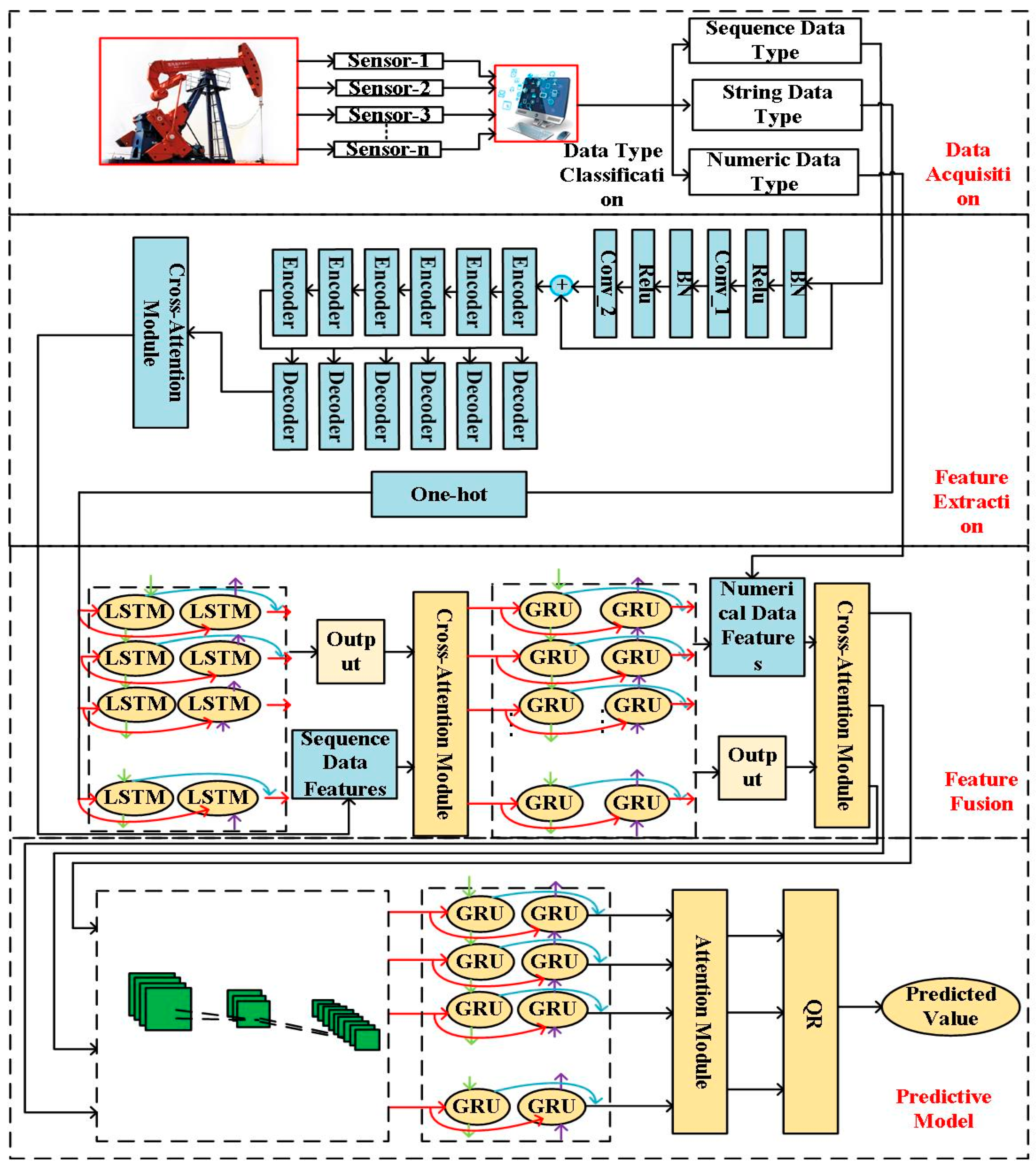
Figure 1. Online prediction model of pumping well system efficiency based on progressive cross-fertilization.
Fractalfract 09 00545 g001
Figure 2. Online prediction model for efficiency of late fusion pumping unit well system based on adaptive weights.
Fractalfract 09 00545 g002
Figure 3. Online prediction model of pumping well system efficiency based on Two-Step Progressive Feature Fusion.
Fractalfract 09 00545 g003
Figure 4. Online prediction model of pumping well system efficiency based on parallel-string cascade integration.
Fractalfract 09 00545 g004
Figure 5. Online prediction model of pumping well system efficiency based on data envelope method.
Fractalfract 09 00545 g005
Figure 6. Online prediction model of pumping well system efficiency based on integration of multiple integration strategies.
Fractalfract 09 00545 g006
Figure 7. Loss curves and test-set prediction results for each model.
Fractalfract 09 00545 g007aFractalfract 09 00545 g007b
Table 1. Components and benefits.
Components Benefits
Feature ExtractionResidual NetworksBy employing multi-layer convolutional stacks with shortcut connections, fine-grained local features across multiple receptive fields are efficiently extracted, while mitigating vanishing gradients and ensuring scalable network depth and performance.
TransformerThis mechanism establishes long-range dependencies, enhancing the model’s perception of global semantic information and compensating for the limited receptive field of pure convolutional networks.
Cross-AttentionDynamic weighted fusion across features from different modalities or hierarchical levels enables alignment and complementarity of critical features, thereby enhancing the discriminative power of the feature representations.
Feature FusionBiLSTMBy capturing contextual information in both the forward and backward directions of the input sequence, it can more comprehensively model bidirectional dependencies.
Cross-AttentionBy computing attention weights across features from different branches or modalities, it enables the complementary alignment of critical features.
BiGRUBy supporting bidirectional propagation, it preserves robust temporal modeling capability while enhancing training efficiency and generalization.
Predictive ModelCNNIt can efficiently capture local spatiotemporal dependencies and feature patterns.
BiGRUBy aggregating information from both the forward and backward directions of the sequence, it fully captures bidirectional dependencies.
AttnetionIt can establish direct dependencies between all positions in a sequence or feature set, thereby overcoming the limitations of recurrent and convolutional networks in capturing long-range information.
Table 2. Components and benefits.
Components Benefits
Feature ExtractionResidual NetworksBy employing multi-layer convolutional stacks with shortcut connections, fine-grained local features across multiple receptive fields are efficiently extracted, while mitigating vanishing gradients and ensuring scalable network depth and performance.
TransformerThis mechanism establishes long-range dependencies, enhancing the model’s perception of global semantic information and compensating for the limited receptive field of pure convolutional networks.
Cross-AttentionDynamic weighted fusion across features from different modalities or hierarchical levels enables alignment and complementarity of critical features, thereby enhancing the discriminative power of the feature representations.
Predictive Model-1CNNIt can efficiently capture local spatiotemporal dependencies and feature patterns.
BiGRUBy aggregating information from both the forward and backward directions of the sequence, it fully captures bidirectional dependencies.
Cross-AttentionDynamic weighted fusion across features from different modalities or hierarchical levels enables alignment and complementarity of critical features, thereby enhancing the discriminative power of the feature representations.
Predictive Model-2CNNIt can efficiently capture local spatiotemporal dependencies and feature patterns.
BiGRUBy aggregating information from both the forward and backward directions of the sequence, it fully captures bidirectional dependencies.
BiLSTMBy capturing contextual information in both the forward and backward directions of the input sequence, it can more comprehensively model bidirectional dependencies.
Table 3. Components and benefits.
Components Benefits
Feature ExtractionResidual NetworksBy employing multi-layer convolutional stacks with shortcut connections, fine-grained local features across multiple receptive fields are efficiently extracted, while mitigating vanishing gradients and ensuring scalable network depth and performance.
TransformerThis mechanism establishes long-range dependencies, enhancing the model’s perception of global semantic information and compensating for the limited receptive field of pure convolutional networks.
Cross-AttentionDynamic weighted fusion across features from different modalities or hierarchical levels enables alignment and complementarity of critical features, thereby enhancing the discriminative power of the feature representations.
Predictive Model-1AttentionIt can establish direct dependencies between all positions in a sequence or feature set, thereby overcoming the limitations of recurrent and convolutional networks in capturing long-range information.
BiGRUBy aggregating information from both the forward and backward directions of the sequence, it fully captures bidirectional dependencies.
BiLSTMBy capturing contextual information in both the forward and backward directions of the input sequence, it can more comprehensively model bidirectional dependencies.
Predictive Model-2BiRNNBy employing both forward and backward hidden states, it comprehensively captures contextual dependencies at both the beginning and end of the sequence.
BiGRUBy aggregating information from both the forward and backward directions of the sequence, it fully captures bidirectional dependencies.
BiLSTMBy capturing contextual information in both the forward and backward directions of the input sequence, it can more comprehensively model bidirectional dependencies.
Table 4. Components and benefits.
Components Benefits
ModelsPCFEThis model seamlessly integrates heterogeneous sensor data through specialized encoders, dynamically fuses multi-scale features via Cross-Attention, and delivers robust real-time efficiency predictions with uncertainty quantification using a GRU–attention–quantile regression pipeline.
AWFEThis model combines specialized encoders for sequence, string, and numeric data with cross-modal attention fusion and ensemble GRU/LSTM predictors, topped by a quantile regression output to deliver robust, real-time efficiency predictions with uncertainty quantification.
TSPEBy employing dedicated encoders for numeric, string, and sequence data with Cross-Attention fusion, and integrating dual-branch GRU/LSTM networks with quantile regression, this model achieves end-to-end multimodal feature fusion, real-time high-precision efficiency prediction, and uncertainty quantification.
Weight OptimizationGKSOBy mimicking sharks’ dynamic foraging strategies, SOA effectively balances exploration and exploitation, reducing the risk of premature convergence to local optima.
Table 5. Components and benefits.
Components Benefits
ModelsPCFEThis model seamlessly integrates heterogeneous sensor data through specialized encoders, dynamically fuses multi-scale features via Cross-Attention, and delivers robust real-time efficiency predictions with uncertainty quantification using a GRU–attention–quantile regression pipeline.
AWFEThis model combines specialized encoders for sequence, string, and numeric data with cross-modal attention fusion and ensemble GRU/LSTM predictors, topped by a quantile regression output to deliver robust, real-time efficiency predictions with uncertainty quantification.
TSPEBy employing dedicated encoders for numeric, string, and sequence data with Cross-Attention fusion, and integrating dual-branch GRU/LSTM networks with quantile regression, this model achieves end-to-end multimodal feature fusion, real-time high-precision efficiency prediction, and uncertainty quantification.
Weight OptimizationDEADEA derives weights directly from the data without assuming a specific functional form, allowing each decision-making unit to be evaluated against its own “best-practice” frontier.
Table 6. Components and benefits.
Components Benefits
ModelsEPCIThe model achieves high-precision, robust system efficiency prediction by adaptively calibrating fusion weights with the Shark Optimization Algorithm to perform weighted integration of two complementary base learners.
EDEABy leveraging Data Envelopment Analysis to optimally compute fusion weights for PCFE, AWFE, and TSPE, this model adaptively integrates three complementary predictors to achieve unbiased, high-accuracy system efficiency forecasts.
Table 7. Data characterization.
CharacteristicsExampleCharacteristicsExampleCharacteristicsExample
Rated power of the electric motor15 KWNumber of centralizers750Well inclination angle0.43, 0.43, 0.58, …
Motor no-load power0.57 KWPump diameter28 mmDogleg severity0, 0.15, 0.29, …
Motor rated efficiency88.5%Stroke frequency3 (min−1)Electrical power curve13, 13.2, 15.6, …
Pump setting depth2250 mNumber of rod string grades2Balancing methodCrank balance
Stroke length2 mEquivalent diameter of rod string17.474 mmPumping unit modelCYJY14-4.8-73HB
Balance degree95%Tubing specification62 mmRelative density of natural gas0.6
Saturation pressure5 MpaSubmergence depth0.8 mTubing pressure0.8 Mpa
Well fluid density815 (kg/m3)Pump clearance grade1Gas–oil ratio25
Well fluid viscosity5 (mPa s)Dynamic fluid level2250 mCasing pressure0.8 Mpa
System efficiency22.34%Water cut35%
Table 8. Evaluation indicators.
MethodsR2 L τ
PCFE0.7961 ± 0.00761.8927 ± 0.0324
AWFE0.7627 ± 0.00712.0835 ± 0.0258
TSPE0.7693 ± 0.00852.0637 ± 0.0966
EPCI0.8685 ± 0.001171.5490 ± 0.0221
EDEA0.8581 ± 0.001141.7357 ± 0.0179
MEIE0.9335 ± 0.001031.2293 ± 0.0073
Table 9. Evaluation indicators.
Model R 2 L τ
PCFE0.7961 ± 0.00851.8927 ± 0.0329
ResNet0.7564 ± 0.01192.0369 ± 0.0882
ResNet–Transformer0.7746 ± 0.01011.9464 ± 0.0596
QRCNN0.7552 ± 0.01552.0388 ± 0.1294
QRCNN-BiGRU0.7734 ± 0.01031.9564 ± 0.0731
Table 10. Percent change for each ablation experiment.
Model Percentage   Change   of   R 2 /% Percentage   Change   of   L τ /%
ResNet2.354.65
ResNet–Transformer2.712.83
QRCNN1.824.21
QRCNN-BiGRU2.853.37
Table 11. Evaluation indicators.
Model R 2 L τ
AWFE0.7923 ± 0.00721.8645 ± 0.0262
ResNet–Transformer0.7756 ± 0.01061.9900 ± 0.0285
QRCNN-GRU-10.7714 ± 0.01111.9904 ± 0.0294
QRCNN-10.75234 ± 0.01462.1569 ± 0.03127
QRGRU-10.7544 ± 0.01512.1369 ± 0.03016
QRCNN-BiLSTM-20.7743 ± 0.01091.9901 ± 0.0291
QRBiLSTM-BiGRU-20.7708 ± 0.00952.0835 ± 0.0233
QRGRU-20.7633 ± 0.01462.1046 ± 0.0332
Table 12. Percent change for each ablation experiment.
Model Percentage   Change   of   R 2 /% Percentage   Change   of   L τ /%
ResNet–Transformer2.116.73
QRCNN-GRU-12.646.75
QRCNN-12.478.37
QRGRU-12.207.36
QRCNN-BiLSTM-22.276.74
QRBiLSTM-BiGRU-22.7211.75
QRGRU-20.971.01
Table 13. Evaluation indicators.
Model R 2 L τ
TSPE0.8362 ± 0.00961.6590 ± 0.0928
ResNet0.7485 ± 0.02262.3321 ± 0.1353
ResNet–Transformer0.7693 ± 0.02242.0637 ± 0.1174
QRBiLSTM-BiGRU-10.7819 ± 0.02211.9403 ± 0.1068
QRBiRNN-BiGRU-20.7715 ± 0.02132.0224 ± 0.1047
QRBiRNN-BiLSTM-20.7823 ± 0.02071.9263 ± 0.1141
QRBiGRU-BiLSTM-20.7708 ± 0.01912.1210 ± 0.1219
QRBiLSTM-10.7706 ± 0.02942.1222 ± 0.1359
QRBiGRU-10.7708 ± 0.03272.0959 ± 0.1446
QRBiRNN-20.7519 ± 0.02512.2361 ± 0.1422
QRBiLSTM-20.7617 ± 0.03042.2094 ± 0.1863
QRBiGRU-20.7507 ± 0.02942.2476 ± 0.1272
Table 14. Percent change for each ablation experiment.
Model Percentage   Change   of   R 2 /% Percentage   Change   of   L τ /%
ResNet2.7113.01
ResNet–Transformer8.0024.40
QRBiLSTM-BiGRU-16.5016.96
QRBiRNN-BiGRU-27.7421.90
QRBiRNN-BiLSTM-26.4516.11
QRBiGRU-BiLSTM-27.8227.85
QRBiLSTM-11.459.38
QRBiGRU-11.428.02
QRBiRNN-22.5010.57
QRBiLSTM-23.8914.70
QRBiGRU-22.615.63
Table 15. Evaluation indicators.
Model R 2 L τ
EPCI0.8685 ± 0.001191.5490 ± 0.0243
PCFE0.7802 ± 0.001521.9058 ± 0.1106
AWFE0.7849 ± 0.001501.9608 ± 0.1757
TSPE0.7320 ± 0.00162.2094 ± 0.1033
Table 16. Percent change for each ablation experiment.
Model Percentage   Change   of   R 2 /% Percentage   Change   of   L τ /%
PCFE10.1723.03
AWFE9.6326.59
TSPE15.7242.63
Table 17. Evaluation indicators.
Model R 2 L τ
EDEA0.8581 ± 0.001061.7357 ± 0.0196
PCFE0.7664 ± 0.001641.9588 ± 0.1114
AWFE0.7850 ± 0.001531.9387 ± 0.1801
TSPE0.7566 ± 0.001582.1500 ± 0.1126
Table 18. Percent change for each ablation experiment.
Model Percentage   Change   of   R 2 /% Percentage   Change   of   L τ /%
PCFE10.6912.85
AWFE8.5211.70
TSPE11.8323.87
Table 19. Valuation metrics.
Model R 2 L τ
MEIE0.9130 ± 0.001031.3002 ± 0.0076
EPCI0.8609 ± 0.001111.5742 ± 0.0238
EDEA0.8581 ± 0.001091.7357 ± 0.0191
Table 20. Valuation metrics.
Model Percentage   Change   of   R 2 /% Percentage   Change   of   L τ /%
EPCI5.716.01
EDEA21.0733.50
Disclaimer/Publisher’s Note: The statements, opinions and data contained in all publications are solely those of the individual author(s) and contributor(s) and not of MDPI and/or the editor(s). MDPI and/or the editor(s) disclaim responsibility for any injury to people or property resulting from any ideas, methods, instructions or products referred to in the content.