Rolling Bearing Fault Diagnosis Based on Fractional Constant Q Non-Stationary Gabor Transform and VMamba-Conv

Abstract

Rolling bearings are prone to failure, meaning that research on intelligent fault diagnosis is crucial in relation to this key transmission component in rotating machinery. The application of deep learning (DL) has significantly advanced the development of intelligent fault diagnosis. This paper proposes a novel method for rolling bearing fault diagnosis based on the fractional constant Q non-stationary Gabor transform (FCO-NSGT) and VMamba-Conv. Firstly, a rolling bearing fault experimental platform is established and the vibration signals of rolling bearings under various working conditions are collected using an acceleration sensor. Secondly, a kurtosis-to-entropy ratio (KER) method and the rotational kernel function of the fractional Fourier transform (FRFT) are proposed and applied to the original CO-NSGT to overcome the limitations of the original CO-NSGT, such as the unsatisfactory time–frequency representation due to manual parameter setting and the energy dispersion problem of frequency-modulated signals that vary with time. A lightweight fault diagnosis model, VMamba-Conv, is proposed, which is a restructured version of VMamba. It integrates an efficient selective scanning mechanism, a state space model, and a convolutional network based on SimAX into a dual-branch architecture and uses inverted residual blocks to achieve a lightweight design while maintaining strong feature extraction capabilities. Finally, the time–frequency graph is inputted into VMamba-Conv to diagnose rolling bearing faults. This approach reduces the number of parameters, as well as the computational complexity, while ensuring high accuracy and excellent noise resistance. The results show that the proposed method has excellent fault diagnosis capabilities, with an average accuracy of 99.81%. By comparing the Adjusted Rand Index, Normalized Mutual Information, F1 Score, and accuracy, it is concluded that the proposed method outperforms other comparison methods, demonstrating its effectiveness and superiority.

1. Introduction

Rolling bearings, as key components of rotating mechanical equipment, are widely used in various industrial devices. Due to the possible influence of factors such as friction, wear, and fatigue during long-term operation, rolling bearings may experience faults. Therefore, studies on fault monitoring and diagnosis in rolling bearings are of extremely high practical value and research significance [1].

Under practical operating conditions, the distinct structural components of a rolling bearing—such as the inner and outer races, rolling elements, and cage—exhibit significant differences in their functions, stress mechanisms, and kinematic characteristics. Consequently, their failure modes and fault origins also vary. Damage to the races and rolling elements primarily originates from rolling contact fatigue under cyclic loading, whereas cage fracture is typically caused by vibrational impacts, wear, or structural problems [2]. These faults, stemming from different physical mechanisms, excite vibrational responses with unique frequency signatures, which provides a theoretical foundation for precise diagnostics. Therefore, to conduct a comprehensive and systematic investigation of bearing failures, this study focuses on five of the most representative health states: the normal condition, and four typical fault types: inner race fault, outer race fault, rolling element fault, and cage fracture.

Traditional fault-diagnosis techniques require manual selection of fault-signal features, depend heavily on expert knowledge, and are easily influenced by human factors, leading to uncertainty in diagnostic results [3]. In recent years, deep learning (DL) has greatly advanced intelligent diagnosis methods thanks to its powerful nonlinear-mapping ability and end-to-end feature-learning capability [4]. Especially in strongly nonlinear, high-noise scenarios such as rolling bearings, deep neural networks can markedly improve diagnostic accuracy and robustness [5]. By converting rolling bearing vibration signals into two-dimensional images, fault features can be automatically extracted, thereby reducing human intervention and enhancing diagnostic efficiency and accuracy. These image-based diagnostic approaches capture fault characteristics in signals more effectively and strengthen diagnostic performance under complex operating conditions and noisy environments [6]. For instance, Wang et al. [7] transformed vibration signals into two-dimensional images and fed them into an improved 2D-CNN, achieving higher diagnostic accuracy than a 1D-CNN.

Most existing fault diagnosis models learn features from the time domain or frequency domain of the signal, which is often not sufficient to meet requirements. Time–frequency domain analysis presents the global characteristics of the signal through joint distribution and can provide more comprehensive diagnostic information [8]. Common time–frequency transformation techniques include short-time Fourier transform (STFT), Wigner–Ville distribution (WVD), and continuous wavelet transform (CWT) [9]. However, these all have inherent flaws: STFT cannot take into account both time and frequency resolution and the window width is fixed; there is a cross-term problem in WVD; and CWT requires the manual selection of wavelet bases. Improper basis functions will affect the processing effect of non-stationary signals. According to the time–bandwidth product theorem, short-time Fourier transform cannot achieve high time resolution while also having high frequency resolution. Moreover, the window width of STFT is fixed and cannot be adjusted adaptively. Although the WVD exhibits excellent symmetry and is highly effective for analyzing linear frequency-modulated signals, it generates problematic cross-term interference when applied to multi-component signals, making the results difficult to interpret. Continuous wavelet transform requires the manual selection of appropriate wavelet basis functions. If the wavelet basis is not properly selected, then the processing effect on non-stationary signals will not be ideal. To solve this problem, Velasco et al. [10] proposed the constant Q non-stationary Gabor transform (CQ-NSGT) with adaptive time and frequency resolution. This transformation can achieve signal reconstruction at a relatively low computational cost and is expected to simultaneously achieve high temporal resolution and high frequency resolution. However, in the original CQ-NSGT, some parameters need to be set manually, including the window function, the number of frequency boxes per octave, and the frequency limit. Among these, the number of frequency boxes per octave has the greatest impact on the time–frequency resolution of CQ-NSGT. For frequency-modulated signals with frequency varying over time, CQ-NSGT still has the problem of energy dispersion, which leads to limitations in processing non-stationary signals. Xie et al. [11] introduced the fractional Fourier transform to convert the time-domain signal into the frequency-domain signal through the fractional Fourier transform, thereby obtaining more detailed frequency characteristic information. Liu et al. [12] proposed a collaborative diagnostic model integrating fractional Fourier transform (FrFT) and error backpropagation (BP) neural networks, which efficiently and effectively enhanced multi-scale feature extraction and representation. Aiming to address the fact that some parameters need to be manually set in the original CO-NSGT, especially the number of frequency boxes per octave, which has the greatest impact on the time–frequency resolution of CQ-NSGT, and there is still the problem of energy dispersion in the face of frequency-modulated signals with frequency varying over time, a new time–frequency transformation method, FCQ-NSGT, is proposed.

Convolutional neural networks (CNNs) and vision transformers (ViTs) are currently the most popular basic models in research on deep learning fault diagnosis. For example, Guo et al. [13] utilized the Markov transfer field to convert the fault signal into a two-dimensional fault graph and inputted it into the MDAN-GhostCNN for fault diagnosis in rolling bearings, achieving a relatively good diagnostic effect. Fan et al. [14] applied empirical mode decomposition combined with the pseudo-Wegener distribution time–frequency conversion algorithm and the improved ViT model to the fault diagnosis of rolling bearings, achieving good results. Li et al. [15] proposed an FO-SDRSN bearing fault diagnosis method, which converted the vibration signal into a two-dimensional time series feature map and inputted it into the SDRSN for fault classification, achieving good results. Hou et al. [16] combined the improved time-frequency transformer and the self-attention mechanism to achieve fault diagnosis in rolling bearings. Although both CNNs and ViTs have achieved remarkable success in the field of fault diagnosis, compared with CNNs, ViTs usually exhibit superior performance, which is mainly attributed to the global receptive field and dynamic weights promoted by the attention mechanism. However, the attention mechanism requires quadratic complexity in the image size, resulting in a large computational overhead [17]. Recently, the visual Mamba class model based on the state-space model (SSM) [18] has received significant attention. It inherits the advantages of CNNs and ViTs and at the same time improves efficiency. It can achieve linear complexity without sacrificing the global receptive field. Applying it to the task of fault diagnosis in rolling bearings could lead to major advantages. Than et al. [19] integrated an attention mechanism into VMamba and utilized few-shot learning to propose a new method named MixMamba-Fewshot. Deng et al. [20] proposed an improved RSMamba network based on multi-domain image fusion for fault diagnosis in wheel-set bearings and achieved very good results. Hue et al. [21] combined convolution with Mamba and proposed a lightweight neural network named ConvMamba for fault diagnosis in rolling bearings, which achieves a high fault identification accuracy rate while maintaining high efficiency. Inspired by the above, this study will explore the potential of the visual state space model in the design of lightweight rolling bearing fault diagnosis models and present our design for a lightweight fault diagnosis framework, VMamba-Conv.

To solve the aforementioned problems, this paper proposes a new lightweight fault diagnosis method for rolling bearings based on FCQ-NSGT and VMamba-Conv. FCQ-NSGT technology converts the vibration signal into a time–frequency fault graph and then inputs it into VMamba-Conv for feature extraction and pattern recognition. The main contents and innovation points of this article are as follows:

(1)

An experimental platform for fault diagnosis of rolling bearings is constructed, and a new lightweight method for fault diagnosis in rolling bearings based on FCQ-NSGT and VMamba-Conv is proposed.

(2)

We propose a kurtosis-to-entropy ratio (KER) method. It is introduced into CO-NSGT, overcoming the limitation of unsatisfactory time–frequency representation caused by manual parameter setting in the original CO-NSGT. By introducing a fractional-order rotation kernel, the rotational alignment of linear or slow frequency modulation features in the signal is effectively achieved, meaning that the energy distribution is highly concentrated and more concentrated features and a higher signal-to-noise ratio are obtained.

(3)

A one-dimensional vibration signal is converted into a two-dimensional time–frequency image through FCO-NSGT, and the fault data set is established.

(4)

A new visual state space model, VMamba-Conv, is proposed and applied to fault diagnosis in rolling bearings. The efficient selective scanning mechanism, state space model, and convolutional network are designed in a lightweight manner based on the dual-branch architecture of SimAX fusion and inverted residual blocks to achieve the extraction of local and global features of faults. It enables VMamba-Conv to achieve linear complexity while retaining the global receptive field and dynamic weights and improves the feature extraction ability.

Comparative experiments were conducted with CNN-class methods, transformer-class methods, and SSM-class deep learning methods. It was verified that the proposed FCQ-NSGT and VMamba-Conv fault diagnosis models have good test accuracy and stability. While significantly improving computational efficiency and achieving a lightweight model, they maintain extremely high fault diagnosis capabilities. They demonstrate excellent thermal break performance and outstanding noise resistance.

The framework of this article is as follows: Section 2 introduces related theories such as FCQ-NSGT, SimAM, VMamba-Conv, efficient 2D selective scanning, a lightweight visual state space, and an inverted residual structure. Section 3 explains the construction of the rolling bearing fault test platform and the data acquisition process; Section 4 elaborates on the rolling bearing fault diagnosis model based on FCQ-NSGT and VMamba-Conv. Section 5 conducts a multi-dimensional analysis of the experimental results and compares them with those of other models. Section 6 presents our conclusions.

2. Basic Principles

2.1. Fractional Constant Q Non-Stationary Gabor Transform

To further improve the time–frequency expression ability for fault characteristics, a new time–frequency transformation method is proposed, namely, the fractional-order constant Q non-stationary Gabor transformation. We also introduce the kurtosis-to-entropy ratio in CQ-NSGT. The rotation kernel function of KER [22,23] and fractional Fourier transform (FRFT) [23] generates time–frequency representation (TFR), which can estimate the amplitude of multi-component non-stationary signals more accurately and achieve high time–frequency energy aggregation. The implementation of FCQ-NSGT is as follows:

(1)

Parameter selection is performed, guided by KER. Since the number of frequency boxes B per octave has the greatest influence on the calculation results of CQ-NSGT, this study only considers the optimal selection of this parameter. Other parameters of CO-NSGT are set as default parameters. Specifically, the default window function is “hann”, the minimum frequency ξ_min is greater than or equal to the ratio of the sampling frequency ξ_s to the signal length N, and the maximum frequency ξ_max is strictly lower than the Nyquist frequency ξ_s/2. Additionally, considering that kurtosis and Rényi entropy can, respectively, describe the impact characteristics and energy concentration related to rolling bearing faults [24], the higher the kurtosis, the more concentrated the time–frequency energy, the stronger the signal impact characteristics; the lower the entropy, the more concentrated the energy distribution, the greater the concentration represented by the time–frequency, the better the aggregation. Compared with the classical Shannon entropy, Rényi entropy can flexibly adjust its sensitivity to the signal energy distribution through the parameter α, making it more suitable for characterizing transient features and energy fluctuations in nonlinear and nonstationary vibration signals. A kurtosis entropy ratio method is proposed. The larger the KER value, the better the comprehensive performance of the impulse characteristics and time–frequency aggregation of the signal. Therefore, the larger its value, the more in line it is with the goals of fault signal analysis and parameter optimization, and it is used to find the optimal parameter B of the original CQ-NSGT. This method is capable of simultaneously measuring the time–frequency resolution and impact fault information of TFR. The KER principle is as follows:

$$\begin{array}{c}TFR = cqt(X,‘\mathrm{Sampling} \mathrm{frequency}’,F_s,‘\mathrm{Number} \mathrm{of} \mathrm{frequency} \mathrm{boxes}’,\\ B,‘\mathrm{Frequency} \mathrm{limitation}’,[{\xi }_{min},{\xi }_{max}])\end{array}$$

(1)

$$Kur(TFR)={\displaystyle \frac{E[{(TFR-\mu )}^4]}{{\sigma }^4}}$$

(2)

$$Re(TFR)={\displaystyle \frac{1}{1-\alpha }}{\log }_2{\displaystyle \frac{{\displaystyle \iint TFR{(t,\omega )}^{\alpha }dtd\omega }}{{\displaystyle \iint TFR(t,\omega )dtd\omega }}}$$

(3)

$$KER=\max {\displaystyle \frac{(Kur(TFR))}{Re(TFR)}},B\mathsf{\in }[B_{\min },B_{\max }]$$

(4)

Here, TFR is the two-dimensional time–frequency representation of the rolling bearing fault signal X, cqt( ) is the mathematical calculation function of CO-NSGT, Kur(TFR) and Re(TFR) are the kurtosis vector and Rényi entropy of the TFR of signal X, respectively, and B represents the number of frequency boxes per harmonic pass, which is an integer between 1 and 96. E( ) represents the mathematical expectation, µ and σ are the mean and standard deviation of signal X, and α is the order of Rényi entropy. A value of $\alpha$ = 3 is selected, as reported in the literature [25], to provide superior performance in mechanical fault diagnosis, a setting that our experimental validation also confirms as appropriate for this work. This method allows for the precise measurement of the time–frequency distribution for most non-stationary signals.

(2)

CQ-NSGT is performed using the selected parameters. The TFR of the above signal is calculated using CQ-NSGT containing the optimal parameter B (the optimal number of frequency boxes per octave).

(3)

The focusing and extraction of the impact signal are achieved by means of the rotation kernel function FRFT, and the most discriminative component is extracted through sparse selection to generate TFR. The principle is as follows:

$${\mathcal{T}}_{\alpha }(u,\omega )={\mathcal{F}}_{\alpha }[TFR(t,\omega )](u)={\displaystyle {\int }_{-\infty }^{\infty }T}FR(t,\omega )K_{\alpha }(t,u)dt$$

(5)

$$A^{*}=\arg {\min }_A{‖Y-\underset{D}{\underbrace{{\left[\mathrm{vec}({\mathcal{T}}_{\alpha })\right]}_{\alpha \in \mathcal{A}}}}A‖}_2^2+\lambda \Vert A{\Vert }_1$$

(6)

$$TF{R}_{\mathrm{final}}(t,\omega )={\displaystyle \sum _{\alpha \in {\mathcal{A}}^{*}}{\mathcal{F}}_{\alpha }^{-1}}[{\mathcal{T}}_{\alpha }(u,\omega )\odot M_{\alpha }^{*}](t,\omega )$$

(7)

Here, $K_{\alpha }(t,u)$ is the rotation kernel function of FRFT, determining the “rotation” angle and transformation form of the fractional domain; $D={\left[\mathrm{vec}({\mathcal{T}}_{\alpha })\right]}_{\alpha \in \mathcal{A}}$ is the dictionary formed by stacking the FRFT eigenvectors $\mathrm{vec}({\mathcal{T}}_{\alpha })$ of all orders $\alpha$. $Y$ is the original feature vector (provided by $TFR(t,\omega )$) and is used as the reconstruction target in sparse representation [26]; $A^{*}$ is the set of the most useful orders retained corresponding to the non-zero entries of the sparse coefficient matrix, and the mask $M_{\alpha }^{*}$ is thus generated. $\odot$ denotes element-wise multiplication. ${\mathcal{F}}_{\alpha }^{-1}$ is the inverse fractional Fourier transform of order a, which is used to project the filtered fractional domain information back to the time–frequency domain.

2.2. The SimAM Principle

The SimAM (Simple Parameter-Free Attention Module) [27] is a parameter-less lightweight attention module based on neuroscience theory. It dynamically generates the channel-space joint attention weights by defining the energy function to identify neurons with strong spatial inhibition. It only requires tensor operations such as mean and variance, without the need for additional parameter learning. The framework is shown in Figure 1, and the energy function is as follows:

$$e_t(w_t,b_t,y,x_i)={(y_t-\widehat{t})}^2+{\displaystyle \frac{1}{M-1}}{\displaystyle \sum _{i=1}^{M-1}(}{y}_0-{\widehat{x}}_i{)}^2$$

(8)

Here, t and $x_i$ represent the estimated values $X\in R^{C\times H\times W}$ of the target neuron and other neurons on the inputted single channel (C, H, and W, respectively, represent the number of channels, height, and width, and R is the set of real numbers). $w_t$ and $b_t$ represent the weights and deviations, respectively, and $M=H\times W$ represents the number of neurons in this channel. The regularization coefficient λ is introduced into the values. The final minimum energy formula is ${\widehat{t}}_i=w_{t}t+b_t$, and ${\widehat{x}}_i=w_t{x}_i+b_t$ are linear transformations of t and $x_i$. Introducing the regularization coefficient into the weights λ, the final minimum energy formula is as follows:

$$e_t^{\ast }={\displaystyle \frac{4({\widehat{\sigma }}^2+\lambda )}{{(t-\widehat{\mu })}^2+2{\widehat{\sigma }}^2+2\lambda }}$$

(9)

Here, the mean value is $\widehat{\mu }={\displaystyle \frac{1}{M}}{\displaystyle \sum _{i=1}^M{x}_i}$, and the variance is ${\widehat{\sigma }}^2={\displaystyle \frac{1}{M}}{\displaystyle \sum _{i=1}^M(x_i-}\widehat{\mu }{)}^2$. The equation indicates that the lower the energy value $e_t^{\ast }$, the greater the difference between the target neuron and the surrounding neurons, indicating that the energy value is inversely proportional to the separability of the target neuron from the remaining neurons. Therefore, the attention parameter is expressed as $1/e_t^{\ast }$. Using the scaling operator instead of addition to refine the features, the enhanced input with the attention mechanism is ultimately obtained as follows:

$$\tilde{X}=sigmoid(1/E)\odot X$$

(10)

In this paper, SimAM is adopted to replace the traditional SqueezeExcitation attention module for the adaptive fusion of local and global features, thereby suppressing redundant information and enhancing the response of key feature regions. While enhancing the feature extraction ability, it enables the model to achieve a lightweight design.

2.3. The Principle of the VMamba-Conv Model

Previously, lightweight models have mainly focused on designs based on CNNs and ViTs. Research on efficient CNNs mainly compresses the original convolution module through methods such as efficient group convolution [28] and lightweight skip join [29]. Efficient ViTs are achieved by integrating ViTs with CNN fusion to achieve lightweighting [30]. However, the lightweighting of ViTs usually comes with the cost of losing global self-attention ability. Due to the $O\left(N^2\right)$ time complexity of global self-attention, its computational and memory costs increase sharply at high resolutions. The ability to perform global self-attention only in local or low-resolution layers hinders the ability to further improve lightweight models.

The Mamba model demonstrates outstanding performance in various tasks such as language modeling and computer vision while reducing the time complexity of global information extraction to ON. Inspired by the VMamba and CNN models, a VMAMBA-CONV model is proposed for fault diagnosis in rolling bearings. A lightweight design is achieved by integrating efficient 2D selective scanning, a state space model, and a convolutional network with a dual-branch architecture and inverted residual blocks.

VMamba-Conv is an efficient and lightweight visual state space model that integrates the advantages of global and local information extraction to solve the trade-off problem between model accuracy and computational efficiency. A four-stage hierarchical structure is adopted, similar to that of the swin transformer (Figure 2), as follows: The inputted fault time–frequency graph is divided into multiple patches, retaining the 2D structure without flattening it into a 1D sequence. Lightweight visual state space (LVSS) blocks and inverted residual blocks are stacked, and finally the recognition results are outputted using the classification module SoftMax.

The core of VMamba-Conv is composed of efficient 2D selective scanning, lightweight visual state space blocks fused by convolution branches, and inverted residual blocks.

2.3.1. Efficient 2D Selective Scanning

In deep neural networks, downsampling through pooling or a step-size volume product can expand the receptive field at a lower computational cost, but this sacrifices spatial resolution. A strategy based on dilated convolution can effectively expand the receptive field while maintaining resolution. Inspired by this, in order to reduce the computational complexity of selective scanning, efficient 2D selective scanning (Efficient 2D Scanning—ES2D) is introduced. The computational complexity of global feature extraction is reduced from $O\left(N\right)$ to $O\left(N/p^2\right)$, while maintaining the global receptive field. The visual selective scanning module is lightweight and extended by implementing jump sampling on each local block on the feature map, as shown in Figure 3. Given the inputted feature map $X\in R^{C\times H\times W}$, instead of performing a full-map cross-scan, the feature map is sampled at skip intervals with a step size p and divided into four selected spatial dimension features ${\left\{O_i\right\}}_{i=1}^4$.

$$X[:,m::p,n::p]\stackrel{scan}{\to }{O}_i$$

(11)

$$SS2D({\left\{O_i\right\}}_{i=1}^4)\to {\left\{\widetilde{O_i}\right\}}_{i=1}^4$$

(12)

$$Y[:,m::p,n::p]\stackrel{merge}{\to }\widetilde{O_i}$$

(13)

Here, $m=\left[{\displaystyle \frac{1}{2}}+{\displaystyle \frac{1}{2}}sin({\displaystyle \frac{\pi }{2}}(i-2)\right]$, $n=\left[{\displaystyle \frac{1}{2}}+{\displaystyle \frac{1}{2}}cos({\displaystyle \frac{\pi }{2}}(i-2)\right]$, m and n are determined by the sine and cosine numbers O, and OER ensures multi-directional coverage. $O_i$, $\widetilde{O_i}\in R^{C\times \frac{H}{p}\times \frac{W}{p}}$, and the operator $[:,m::p,n::p]$ indicates the slicing of the feature matrix of each channel, starting from m along height H and from n along width W and sampling at intervals of p steps. This process decouples the full scanning method into local and global sparse forms. The skip sampling of the local receptive field reduces the computational complexity by selectively scanning small areas of the feature map. When the step size p is set, the dimension of the sampling feature block is reduced from $(C,H,W)$ as in SS2D to $(C,H/p,W/p)$, reducing the number of tokens processed in each round of scanning and merging operations from N to N/p², significantly improving the efficiency of feature extraction. Global spatial feature map reorganization integrates the processed feature blocks to reconstruct the global structure of the feature map, ensuring local details while retaining the global context information.

While efficiently scanning and merging the module, this design retains the global integration advantage of the state space architecture. By periodically sampling feature map blocks and reorganizing them, it balances local details and the global context, reduces redundant calculations, and ensures comprehensiveness in spatial axis feature extraction.

2.3.2. Lightweight Visual State Space

The lightweight visual state space module adopts a dual-path design, as shown in Figure 4. It achieves complementary advantages while maintaining computational efficiency by collaboratively integrating global and local features. This module replaces the traditional SE attention mechanism with SimAM. Global fault information is obtained through the ES2D module improved via SimAM, local features are extracted in combination with convolutional branches, and dual-path feature representation is optimized after enhancement using SimAM.

ES2D intelligently jumps to scanning feature maps with a step size of p, reducing redundant calculations while maintaining global representation. When dealing with local representations as the main approach, convolution operations demonstrate superior feature extraction capabilities and low computational resources. The parallel convolution branch adopts a 3 × 3 convolution kernel with a step size of 1, as shown in Figure 5, which is specifically used to capture fine-grained local features of faults. Subsequently, the SimAM module adaptively fuses features through the parameter-free energy function and dynamically optimizes the joint attention weights of channels and spaces, enabling the network to efficiently balance the local and global receptive field weights.

The outputs of each SimAM module are feature refined and fused through scaling operators. This dual-path structure can be expressed as follows:

$$X^{l+1}=SimAM(ES2D(X^l))+SimAM(Conv(X^l))$$

(14)

Here, X is the feature map of l layers, and $SimAM(·)$ is a parameter-less joint attention operation. By deploying the SimAM module for each independent path, LVSS can dynamically adjust the feature weights of global information and local information, significantly enhancing the model’s focusing ability on key features. This fusion aims to fully preserve the global characteristics and local fine-grained details of the fault signals of rolling bearings, thereby enhancing lightweight and fault diagnosis capabilities.

2.3.3. Inverted Residual Structure

The efficiency of convolution operation is superior to that of global modeling modules such as transformers. Existing lightweight models typically adopt a “pre-local-post-global” design: in the previous stage, efficient convolution is used to compress the number of tokens to reduce complexity, and in the subsequent stage, a transformer with a complexity of O (N²) is introduced to obtain global information. Under the state space model, the computational complexity of global representation is only O (N), and local modules can be flexibly deployed. The Inverted Residuals (InRes) structure originated from the MobileNetV2 model. By optimizing the information flow and reducing the computational complexity, InRes enables MobileNetV2 to achieve better accuracy while maintaining a lower number of parameters and computational load [31]. Inspired by the MobileNetV2 model, the InRes structure is introduced in the model in this paper: in the first two stages, LVSS blocks are used for global representation modeling, and in the subsequent stages, local feature maps are extracted through InRes(X^l). The formula is as follows:

$$X^{l+1}=\left\{\begin{array}{ll}LVSS(X^l)\hfill & \mathrm{if} X^l\in \left\{\mathrm{Stage}1, \mathrm{Stage}2\right\};\hfill \\ InRes(X^l)\hfill & \mathrm{Other}.\hfill \end{array}\right.$$

(15)

Here, $X^l$ represents the feature map of Layer l, which significantly improves the computing and memory efficiency.

3. Experimental Platform

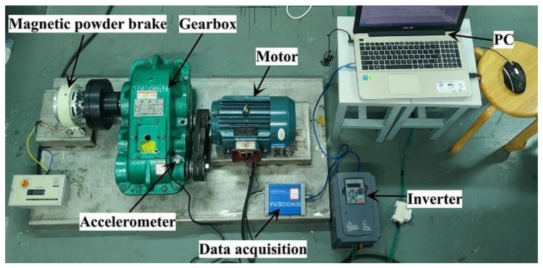
The rolling bearing fault test platform established in this paper is mainly composed of components such as the YE3-100L2-4 three-phase asynchronous motor, the JZQ250 gearbox, the YE6231 data acquisition card, the G7R5/P011T4 frequency converter, the CAYD051V piezoelectric acceleration sensor, and the magnetic powder brake, as shown in Figure 6. The three-phase induction motor combined with a frequency converter was selected because this configuration provides precise speed regulation and stable operation. A magnetic powder brake is used as the load so that a smooth and repeatable torque can be applied without inducing premature thermal failure, ensuring the comparability of fault features at different rotational speeds. The gearbox introduces background vibration and gear meshing harmonics closer to an actual transmission chain, thereby allowing us to test the robustness of the algorithm under non-ideal conditions. The piezoelectric accelerometer, with its wide bandwidth and high sensitivity, is mounted at an axial position on the gearbox to capture the energy of impacts transmitted by the rolling elements while reducing the risk of saturation from local structural resonances. The parameters of the three-phase induction motor are listed in

Table 1. Specific parameters of YE2-100L2-4 three-phase asynchronous motor (Zhejiang Dagao Electric Motor Co., Ltd., Taizhou, China).

Model Number	Infinity	Rated Voltage/V	Rated Rotational Speed/(r∙min−1)	Rated Power	Rated Torque/(N∙m)	Power Factor P.F
YE3-100L2-4	4	380	1440	3	19.9	0.82

.

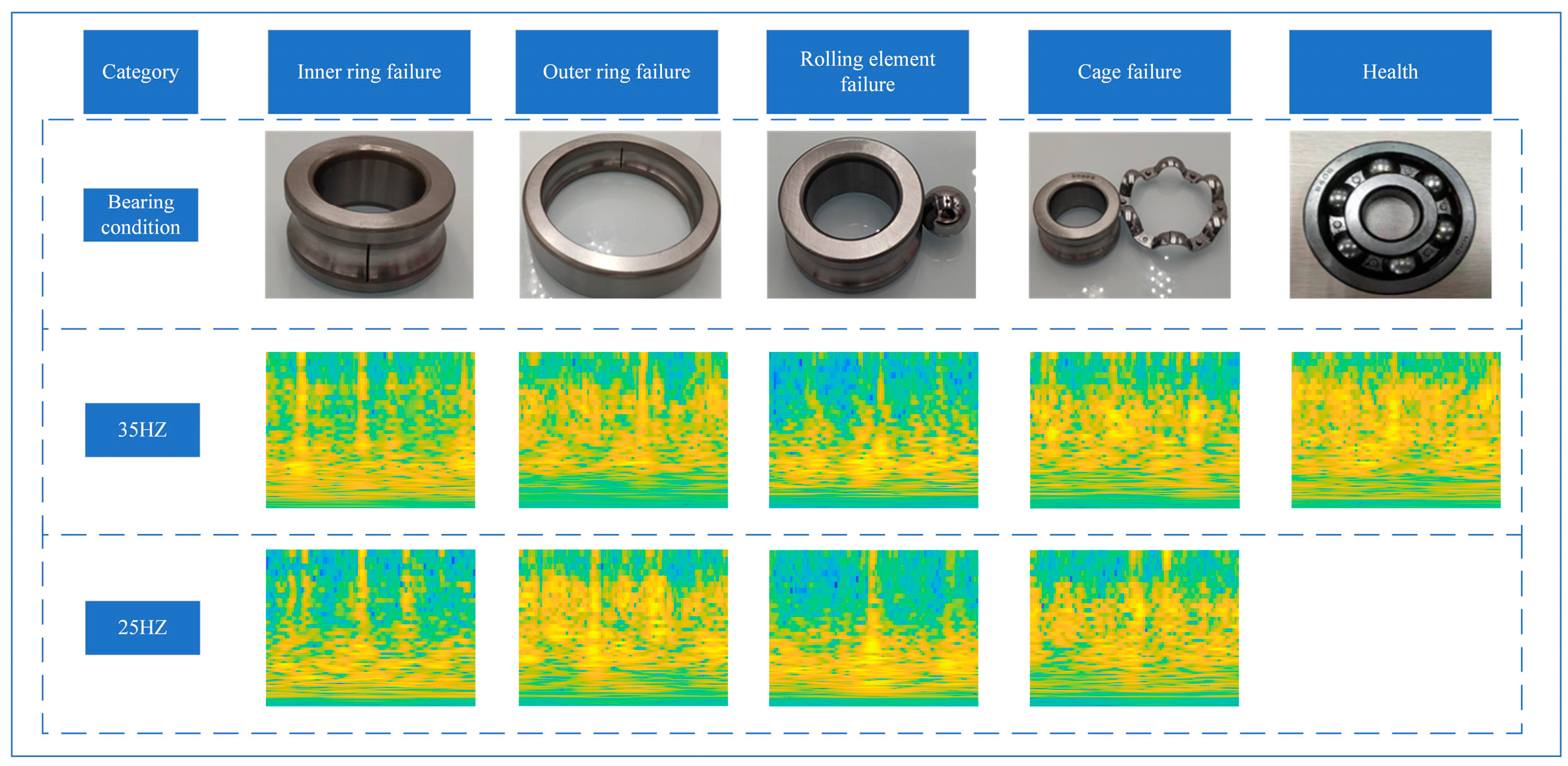
Given that common faults in rolling bearings occur in the inner ring, outer ring, rolling elements and cage, in this experiment, we designed five healthy states, namely, inner ring fault, outer ring fault, rolling element fault, cage fracture, and normal state [32]. The processing was carried out using laser and electrical discharge technology: the inner and outer rings were made of 0.6 × 0.4 mm linear flaking, the rolling elements were slightly pitted, and the cage was slightly broken, as shown in Figure 7, specifically.

In this experiment, multi-condition faults were simulated under a load of 0.5 hp and two rotational speed conditions (750 r/min and 1050 r/min), with continuous sampling triggered at regular intervals using a sampling frequency (Fs) of 12 kHz. A magnetic powder brake with a load setting of 0.5 hp was selected to ensure stable operation under moderate load conditions, preventing significant temperature increases and avoiding premature thermal failure or abnormal nonlinear vibrations, thus enhancing the repeatability and comparability of fault features. The frequency converter was set to frequencies of 25 Hz and 35 Hz, corresponding, respectively, to rotational speeds of 750 r/min and 1050 r/min. These two speeds were selected to analyze how bearing fault characteristics vary under different operating conditions, thus enhancing the generalizability of the collected data set. The fault object—a type 6406 rolling bearing—was installed on the high-speed shaft of the gearbox, with the accelerometer positioned axially on the gearbox to capture high-frequency impact vibrations resulting from localized bearing faults with high sensitivity. Under these two speed conditions (750 r/min and 1050 r/min), five bearing health states were simulated, including inner-race fault, outer-race fault, rolling-element fault, cage fault, and a healthy state. Each state consists of 500 samples, and each sample comprises 2048 data points. The reason for selecting 2048 data points per sample was to achieve a frequency resolution of about 6 Hz, balancing frequency-domain analysis precision with computational efficiency during model training. The data set was divided into training, validation, and testing sets using the commonly adopted ratio of 7:1.5:1.5 [33], with the specific partition details provided in

Table 2. Data partitioning.

Fault Status	Rotational Speed (r/min)	Label	Length	Training Set	Verification Set	Test Set	Sampling Frequency (Hz)
Inner ring fault	750	0	2048	350	75	75	15 K
Outer ring fault	750	1	2048	350	75	75	15 K
Rolling element fault	750	2	2048	350	75	75	15 K
Cage fracture	750	3	2048	350	75	75	15 K
Inner ring fault	1050	4	2048	350	75	75	15 K
Outer ring fault	1050	5	2048	350	75	75	15 K
Rolling element fault	1050	6	2048	350	75	75	15 K
Cage fracture	1050	7	2048	350	75	75	15 K
Normal	1050	8	2048	350	75	75	15 K

.

4. Rolling Bearing Fault Diagnosis Process Based on FCQ-NSGT and VMamba-Conv

The lightweight fault diagnosis method for rolling bearings based on FCQ-NSGT and VMamba-Conv proposed in this paper mainly includes modules such as signal acquisition, data preprocessing, parameter optimization, image transformation, feature extraction, and fault classification. The entire fault diagnosis process is shown in Figure 8.

The specific fault diagnosis steps are as follows:

(1)

Piezoelectric acceleration sensors are used to collect fault signals of rolling bearings on the comprehensive experimental platform for rolling bearings.

(2)

Standardized preprocessing is carried out on the collected fault signals.

(3)

The kurtosis entropy ratio is introduced into CQ-NSGT to obtain the optimal B and then fractional-order and sparse representation are performed to obtain the two-dimensional time spectrum of the sparsest and most discriminative fractional-order features. The FCO-NSGT method is adopted to convert the fault signal into a two-dimensional time–frequency graph, which is randomly sampled and finally divided into the training data set, the verification data set, and the test data set.

(4)

The VMamba-Conv model is constructed, and the training parameters of the model are initialized. The time–frequency graph is input into VMamba-Conv for feature extraction and fault identification. Based on EMA, the training set is input into the VMamba-Conv model for training. The validation set is used to continuously optimize the model parameters until the iteration is complete and the trained model is obtained.

(5)

The test set is inputted into the trained VMamba-Conv model to complete fault diagnosis for rolling bearings and obtain the diagnosis results.

The parameters of the VMamba-Conv model are shown in

Table 3. VMamab-Conv model parameters.

Patch Size	MLP Ratio	SSM d_State	SSM Ratio	SSM_Conv	Step_Size	Dims
4 × 4	4.0	16	2.0	3.0	2.0	24

. Setting a smaller Patch Size will increase the model’s sensitivity to the local information of the image. The MLP ratio is the ratio of the hidden layer dimension of the MLP layer to the input dimension, SSM d_State is the hidden state dimension of SSM, the SSM ratio is the internal channel expansion ratio of the SSM module, and SSm_conv is the kernel size of the depth-separable convolution in the SSM module. Step_Size is the mesh step size (control sequence length) during SSM scanning, and Dims is the reference value for the number of channels at each stage of the model.

5. Experimental Verification and Analysis

For the experiment in this paper, we adopted the Pytorch deep learning framework on the Linux-Ubuntu22.04 system. We set the Batchsize to 64 and the number of iterations to 50 times, adopted the cosine annealing learning rate adjustment strategy, set the gradient cropping threshold to 0.5, set the initial learning rate to 0.001, set the optimizer to AdamW, set the EMA index to 0.999, and enabled automatic mixed precision technology for training to accelerate the calculation and save video memory. To account for the inherent randomness of the model, all comparative experiments were independently repeated 10 times. All performance metrics (Adjusted Rand Index, Normalized Mutual Information, F1 Score, Accuracy) represent the average values from these 10 independent trials to ensure the reliability of the results.

5.1. Time–Frequency Image Acquisition

To verify the time–frequency representation ability of the proposed FCQ-NSGT method, a non-stationary continuous example signal X was constructed for analysis, with the sampling frequency set to 1000 Hz. The formula of the simulated signal is as follows:

$$\left\{\begin{array}{l}{X}_1=\sin (50\pi \mathrm{t})+\sin (100\pi t)+\sin (200\pi t),0\le t\le 4\hfill \\ X_2={\displaystyle \frac{{(t-4)}^2}{8}}\times \sin (400\pi t),0\le t\le 4\hfill \\ X_3=\left\{\begin{array}{l}[{(t-2)}^2/8]\times \sin \left(800\pi t\right),0\le t\le 2\\ 0,2<t\le 4\end{array}\right.\hfill \\ X=X_1+X_2+X_3+0.5\times n(t),0\le t\le 4\hfill \end{array}\right.$$

(16)

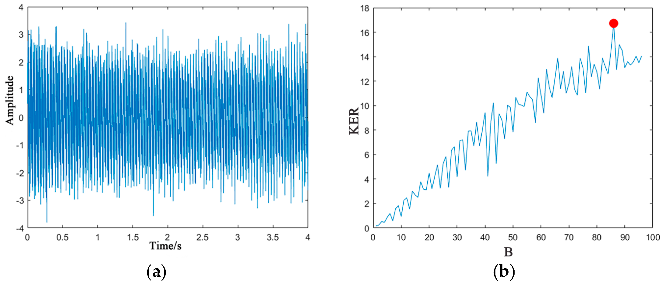
Here, $X_1$ is the superposition of 25 Hz, 50 Hz, and 100 Hz sine waves, $X_2$ and $X_3$ are 200 Hz and 400 Hz sine waves with different amplitude decays; $n(t)$ is a Gaussian white noise component superimposed on three deterministic signals to simulate noise interference in real environments, generated by the MATLAB 2022 function $randn(\cdot )$. Figure 9a shows the time-domain waveform of the sample signal and the result of the time frequency conversion.

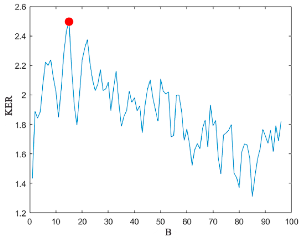
Figure 9b shows that in sample signals, when the number of frequency boxes per octave B reaches 86, the KER reaches the maximum value of 16.8. That is, the optimal number of frequency boxes is 86. By comparing Figure 9c,d, it can be seen that the TFR energy distribution of FCQ-NSGT is more concentrated than that of the original CQ-NSGT, especially the high-frequency components marked by the red box (corresponding, respectively, to signals $X_1$, $X_2$, and $X_3$ ), indicating that its time–frequency representation ability is better. This preliminarily verifies the effectiveness of FCQ-NSGT in time–frequency transformation. The KER graph of the rolling bearing fault signal in Figure 10 shows that when the number of B-frequency boxes per octave is 15, the KER reaches the maximum value of 2.5, and the optimal number of frequency boxes is determined to be 15.

The FCQ-NSGT is adopted to perform time–frequency conversion on the preprocessed vibration signal of the rolling bearing, converting the one-dimensional vibration signal into the FCQ-NSGT time–frequency graph, as shown in Figure 11.

5.2. Result Analysis

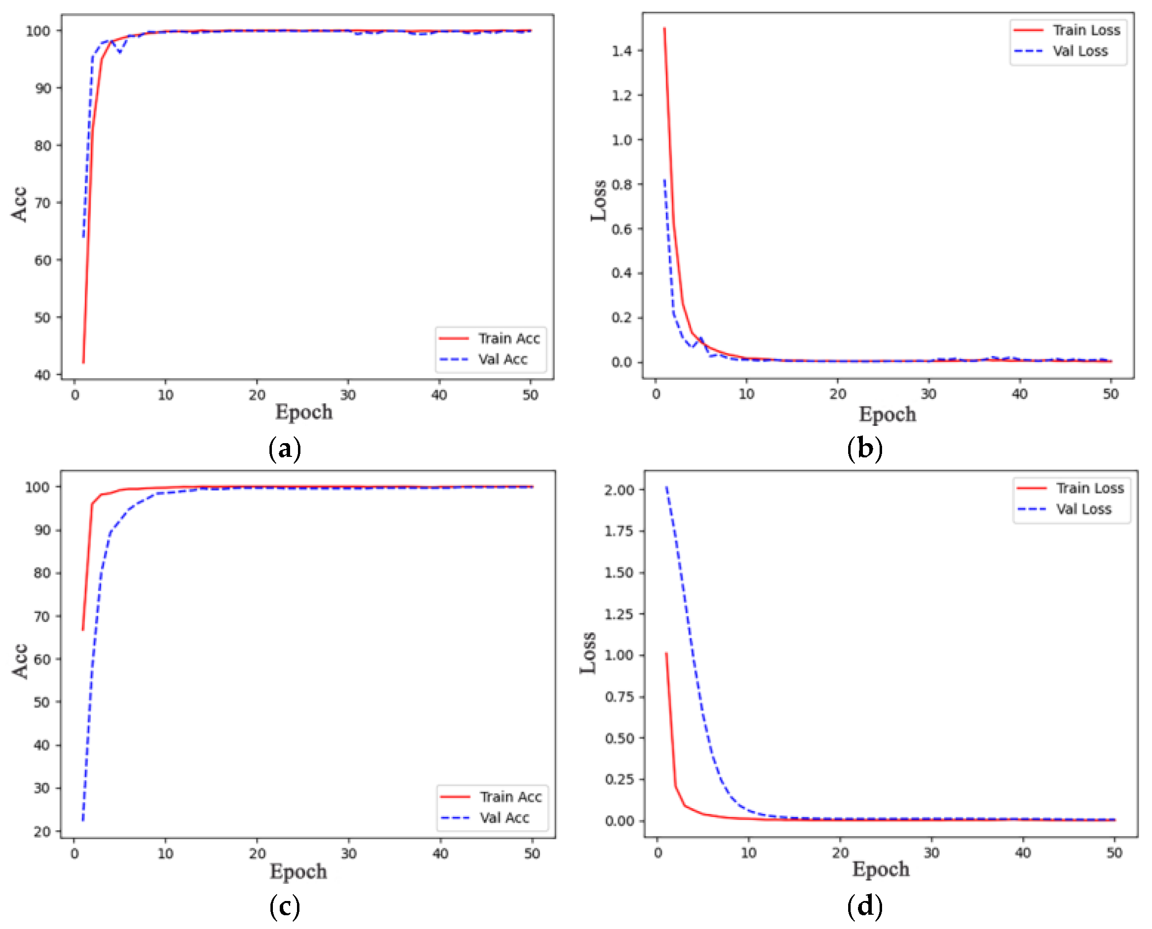
The fault features of the FCQ-NSGT time–frequency graph are extracted through VMamba-Conv. After the training of the VMamba-Conv model, the fault classification results are obtained. Figure 12 shows the iterative curves of the model’s accuracy and loss on the training and validation sets. It can be seen that EMA significantly improves the generalization ability of the model. Without the use of EMA, the convergence performance of the model is very good. However, the performance on the training set and the validation set still fluctuates. Compared with the iterative curve of CQ-NSGT, the fluctuation is reduced, further demonstrating the effectiveness of FCQ-NSGT. After the use of EMA, the curve fluctuation significantly improves, and the convergence speed is not affected. This indicates that EMA effectively improves the generalization ability of the model by smoothing the model weights, making the model perform more stably on the validation set. Therefore, EMA plays a positive role in improving model generalization and alleviating overfitting cooperation and is particularly crucial when dealing with complex tasks.

The training accuracy graph (c) shows that the training accuracy of the model rapidly approaches 100% within the first 10 epochs, indicating the rapid learning and good fitting of data features. The verification accuracy rate has simultaneously increased to nearly 100%, and the curves of the two almost overlap, indicating that the model has no overfitting, has a strong generalization ability, and can adapt to new data.

The training loss graph (d) shows that the training loss of the model drops rapidly and approaches 0 in the first 20 epochs, with a fast fitting speed and low prediction error. The verification loss decreases simultaneously and tends to be stable, indicating that the model performed stably and effectively on the verification set. Overall, the model achieves high accuracy and low loss in fault diagnosis in rolling bearings and has practical application value.

To demonstrate the diagnostic results of the model for rolling bearing faults, the classification confusion matrix of the test set is shown in Figure 13. The classification accuracy for categories 0–6 and 10 (inner ring, outer ring, rolling element faults at 25 Hz/35 Hz, cage fracture (25 Hz) and normal state) reached 100%, indicating that the model has extremely high accuracy for such faults. Only category 7 (35 Hz cage fracture) had a misclassification rate of 1.33% (misjudged as 25 Hz rolling element failure), with an accuracy rate of 98.67%. Category 8 (normal state) has no misclassification, demonstrating the model’s effective distinction between normal and faulty states. The average recognition accuracy rate of multiple experiments was 99.85%, verifying the validity of the model in this paper.

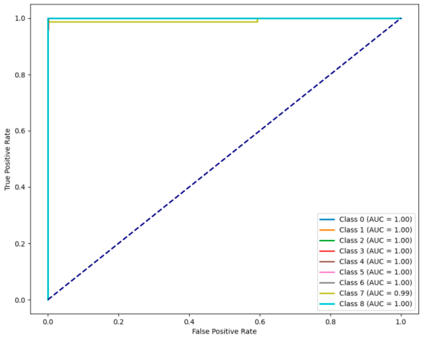
In order to reflect the different false-positive rates (FPRs) and true-positive rates (TPSs) for various categories under the effect of classification, in this paper, we performed ROC curve (receiver operating characteristic curve) analysis on the proposed model, as shown in Figure 14.

Figure 14 shows that, except for category 7 (35 Hz cage fracture, AUC = 0.99), the AUC values for the remaining categories are all close to 1, indicating that the model has an excellent classification effect for most faults, but the discrimination ability for this category is slightly weak. The ROC curves for all categories are far from the randomly guessed diagonal and rapidly approach the upper left corner, verifying that the model has high accuracy and reliability in fault diagnosis and can effectively distinguish various fault states.

To verify the robustness of the method proposed in this paper under strong noise, Gaussian white noise with an SNR of 0 dB, −5 dB, −10 dB, and −15 dB was added to the collected signal [34]. The diagnostic results are shown in Figure 15. Under a low signal-to-noise ratio ranging from 0 dB to −15 dB, the classification accuracy of the method still remains at a relatively high level and the accuracy decreases slowly with the reduction in the signal-to-noise ratio, verifying its excellent anti-noise performance and classification ability.

5.3. Ablation Experiment

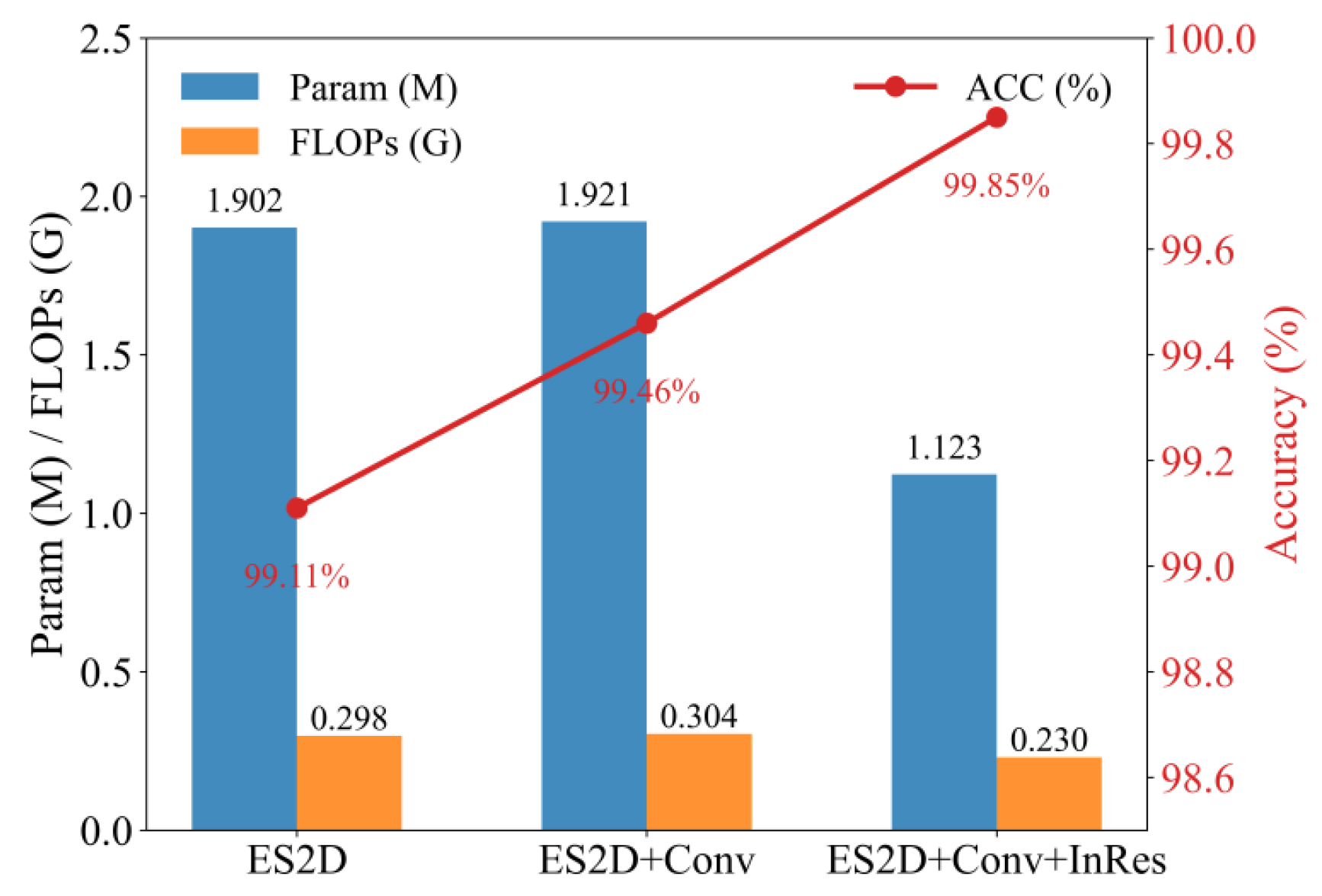
To verify the effectiveness and efficiency of the method proposed in this paper, the effects of ES2D and SimAM in enhancing convolutional branches and inverted residual blocks were analyzed through ablation experiments.

Table 4. Ablation experiment results.

Method	ES2D	ES2D-Conv	InRes	Parameters (M)	FLOPs (G)	ACC (%)
VMamba-Conv	√	×	×	1.902	0.298	99.11
	√	√	×	1.921	0.304	99.46
	√	√	√	1.123	0.230	99.85

and Figure 16 show the results of the ablation experiments (FLOPs and parameter count calculated in the THOP library). The results show that the progressive integration of each module significantly improves diagnostic accuracy while maintaining a low computational complexity.

Figure 16 shows that when using only the ES2D module, the model achieves an accuracy rate of 99.11% with parameters of 1.902M and 0.298GFLOPs, verifying that skip sampling can reduce the computational complexity while maintaining the ability for global feature extraction. After adding convolutional branches and SimAM blocks, the accuracy rate increased to 99.46%, indicating that local feature extraction and ensemble fusion can enhance generalization. The inverted residual module is introduced in the last two stages. Through hierarchical feature allocation (SSM global modeling for shallow high-resolution layers and InRes extraction of local features for deep low-resolution layers), the accuracy rate is increased to 99.85% without increasing parameters. Experiments have proven that the progressive integration of ES2D, Conv, SimAM, and InRes achieves a balance between accuracy and efficiency with linear complexity, providing a new idea for the optimization of lightweight visual models in fault diagnosis.

5.4. Comparative Analysis

To highlight the advantages of the proposed method, multi-index comparisons were conducted with typical deep learning models such as FCQ-NSGT-ConvNeXt, FCQ-NSGT-ViT, FCQ-NSGT-ViM, and CQ-NSGT-VMamba (covering CNN, transformer, and SSM classes) on the same diagnostic cases. After ten repeated experiments, the mean was taken and the error was calculated. The Adjusted Rand Index, Normalized Mutual Information, F1 Score, and accuracy rate were used for evaluation. The results show that the method proposed in this paper is significantly superior to the comparison methods in all indicators, verifying its strong performance in fault diagnosis.

It can be seen from

Table 5. Fault diagnosis results of rolling bearings by different methods.

Method	Evaluation Index
	Adjusted Rand Index	Normalized Mutual Information	F1 Score	Accuracy Rate
FCQ-NSGT-ConvNeXt	0.9770	0.9790	0.9894	0.9895
FCQ-NSGT-ViT	0.9588	0.9616	0.9813	0.9813
FCQ-NSGT-ViM	0.9778	0.9784	0.9903	0.9904
CQ-NSGT-VMamba	0.9875	0.9862	0.9945	0.9945
The method in this article	0.9969	0.9967	0.9985	0.9985

that the method proposed in this paper (FCQ-NSGT-VMamba-Conv) performs the best in all evaluation indicators and the deviation of the evaluation value is also relatively small. Specifically, compared with other advanced CNN-class, transformer-class, and SSM-class methods, it shows improvement by 0.94–3.81%, 1.05–3.51%, 0.40–1.72%, and 0.40–1.72%, respectively, for the ARI, NMI, F1, and ACC indicators, which proves its effectiveness and superiority. The FCO-NSGT-ViM and FCO-NSGT-ViT in this paper show improvements for all four indicators compared with CQ-NSGT-ViT and co-NSGT-VIM, proving that CO-NSGT offers improved efficiency and a better representation ability for time–frequency fault characteristics, greatly improving the performance of the model.

To further compare the feature extraction capabilities of the methods, the features outputted by the test sets in the five methods are visualized in two dimensions using T-SNE, as shown in Figure 17.

As shown in Figure 17, the original data features are scattered and the categories overlap severely, making it impossible to identify the fault type. After extracting features and training using the method proposed in this paper, the degree of feature dispersion and overlap in the T-SNE graph has been significantly improved, whereby the normal state (Class 8) and the fault state are significantly separated, and the features of different types of faults show obvious clustering with only a small amount of local overlap (for example, Class 7 is mistakenly classified as Class 3, as circled in Figure 17f). Compared with other methods, the feature distribution of the method proposed in this paper is more compact and uniform with less overlap, verifying that the model in this paper has a strong feature extraction ability in fault diagnosis in rolling bearings, providing reliable support for practical applications.

It can be seen from

Table 6. Lightweight performance analysis of the model.

Method	FLOPs (G)	Parameters (M)	ACC (%)
CQ-NSGT-VMamba	0.561	3.607	99.45
FCQ-NSGT-VMamba	0.561	3.607	99.91
The method in this article	0.230	1.123	99.85

and Figure 18 that the method proposed in this paper is significantly superior to CO-NSGT-VMamba and FCQ-NSGT-VMamba in terms of computational complexity (FLOPs) and parameters (Parameters), as calculated through the THOP library. The FLOPs decreased from 0.561 G to 0.230 G, and the number of parameters decreased from 3.607 M to 1.123 M. Meanwhile, the classification accuracy (ACC) of the method proposed in this paper reached 99.85%, which is almost on par with the 99.91% of FCQ-NSGT-VMAMBA and superior to the 99.45% of CQ-NSGT-VMAMBA. Compared with CQ-NSGT, FCQ-NSGT improved by 0.46%, further highlighting the level of improvement seen using the FCO-NSGT. The results show that the method proposed in this paper significantly improves computational efficiency of the model and allows it to be more lightweight while maintaining extremely high fault diagnosis performance. It is suitable for scenarios with limited computing resources and effectively guarantees accuracy and rapidity in fault diagnosis.

6. Summary

This paper proposes a new method for fault diagnosis in rolling bearings based on fractional constant Q non-stationary Gabor transform and VMamba-Conv. The results show that the method proposed in this paper has an excellent fault diagnosis ability, with an average accuracy rate reaching 99.85%. Through comprehensive experimental verification and performance evaluation, the contributions and innovation points of this study can be summarized as follows:

(1)

A fractional constant Q non-stationary Gabor transform method is proposed to solve the problems of calculation errors in the original CQ-NSGT, the imperfect time–frequency representation caused by manual parameter setting, and energy dispersion still existing in the face of frequency modulation signals with frequencies that vary with time.

(2)

The results show that the method proposed in this paper improves the indicators of ARI, NMI, F1, and ACC by 0.94–3.81%, 1.05–3.51%, 0.40–1.72%, and 0.40–1.72%, respectively, compared with the control methods. Moreover, the computational complexity and the number of parameters are reduced by approximately 59% and 69%, respectively, compared with CQ-NSGT-VMamba and FCQ-NSGT-VMamba. Its average classification accuracy rate reaches 99.85%, which is close to the 99.91% seen for FCQ-NSGT-VMAMBA and is superior to the 99.45% seen for CQ-NSGT-VMAMBA. Moreover, FCQ-NSGT shows an improvement of 0.46% compared with CQ-NSGT. This method not only improves the computational efficiency of the model and makes it more lightweight, but also shows high diagnostic performance and noise resistance, opening up new possibilities for the application of lightweight state space vision models in fault diagnosis in rolling bearings.

Although the diagnostic results of this study are very good, there are still certain limitations. The method that we propose has currently only been studied and applied under offline conditions in the laboratory and cannot yet be used for online real-time monitoring. In the future, we will monitor the status of rolling bearings in real time online and achieve the early prediction of faults through deep learning models. We also hope to apply this experimental theory to engineering practice.

References

1. Xie, F.; Li, G.; Liu, H.; Sun, E.; Wang, Y. Advancing Early Fault Diagnosis for Multi-Domain Agricultural Machinery Rolling Bearings through Data Enhancement. Agriculture 2024, 14, 112. [Google Scholar] [CrossRef]
2. Peng, B.; Bi, Y.; Xue, B.; Zhang, M.; Wan, S. A Survey on Fault Diagnosis of Rolling Bearings. Algorithms 2022, 15, 347. [Google Scholar] [CrossRef]
3. Liu, R.; Yang, B.; Zio, E.; Chen, X. Artificial intelligence for fault diagnosis of rotating machinery: A review. Mech. Syst. Signal Process. 2018, 108, 33–47. [Google Scholar] [CrossRef]
4. Peng, H.; Zhang, H.; Fan, Y. A review of research on wind turbine bearings’ failure analysis and fault diagnosis. Lubricants 2022, 11, 14. [Google Scholar] [CrossRef]
5. Xie, F.; Wang, Y.; Wang, G.; Sun, E.; Fan, Q.; Song, M. Fault Diagnosis of Rolling Bearings in Agricultural Machines Using SVD-EDS-GST and ResViT. Agriculture 2024, 14, 1286. [Google Scholar] [CrossRef]
6. Wang, C.; Sun, Y.; Wang, X. Image Deep Learning in Fault Diagnosis of Mechanical Equipment. J. Intell. Manuf. 2024, 35, 2475–2515. [Google Scholar] [CrossRef]
7. Wang, J.; Zhang, Q.; Li, Y.; Zhang, T.; Zhang, H. Fault Diagnosis of Bearings Based on Multi-Sensor Information Fusion and 2D Convolutional Neural Network. IEEE Access 2021, 9, 23717–23725. [Google Scholar] [CrossRef]
8. Wang, L.; Qin, Z.; Zhang, Z.; Zhang, J. Free Metaplectic K-Wigner Distribution: Uncertainty Principles and Applications. Fractal Fract. 2025, 9, 245. [Google Scholar] [CrossRef]
9. Bhat, M.Y.; Dar, A.H.; Nurhidayat, I.; Pinelas, S. An Interplay of Wigner–Ville Distribution and 2D Hyper-Complex Quadratic-Phase Fourier Transform. Fractal Fract. 2023, 7, 159. [Google Scholar] [CrossRef]
10. Ding, S.; Chen, R.; Huang, Y.; Wang, X.; Li, J. Application of Reparametric VGG Network in Rolling Bearing Fault Diagnosis. J. Vib. Shock 2023, 42, 313–323. [Google Scholar]
11. Huo, J.; Li, Y.; Chang, C.; Zhang, L.; Wang, Q. Rolling Bearing Fault Diagnosis Based on Hybrid Clipping Unbalanced Data Enhancement and SwinNet Network. J. Vib. Shock 2019, 43, 64–74. [Google Scholar]
12. Wang, S.; Feng, Z. Multi-sensor fusion rolling bearing intelligent fault diagnosis based on VMD and ultra-lightweight GoogLeNet in industrial environments. Digit. Signal Process. 2024, 145, 104306. [Google Scholar] [CrossRef]
13. Guo, J.; Tan, B.; Wang, Z. Fault Diagnosis Method of Rolling Bearing Based on MDAM-GhostCNN. J. Beijing Univ. Aeronaut. Astronaut. 2025, 51, 1172–1184. [Google Scholar]
14. Zhang, H.; Liu, Y.; Wang, J.; Li, Q.; Chen, R. Intelligent Fault Diagnosis of Rolling Bearing Based on EMDPWVD Time-Frequency Image and Improved ViT Network. J. Vib. Shock 2024, 24, 1234–1247. [Google Scholar]
15. Li, T.; Wu, X.; Luo, Z.; Chen, Y.; He, C.; Ding, R.; Zhang, C.; Yang, J. A Bearing Fault Diagnosis Method under Small Sample Conditions Based on the Fractional Order Siamese Deep Residual Shrinkage Network. Fractal Fract. 2024, 8, 134. [Google Scholar] [CrossRef]
16. Hou, Y.; Wang, J.; Chen, Z.; Ma, J.; Li, T. Diagnosisformer: An efficient rolling bearing fault diagnosis method based on improved transformer. Eng. Appl. Artif. Intell. 2023, 124, 106507. [Google Scholar] [CrossRef]
17. Li, J.; Wang, C.; Su, W.; Ye, D.; Wang, Z. Uncertainty-Aware Self-Attention Model for Time Series Prediction with Missing Values. Fractal Fract. 2025, 9, 181. [Google Scholar] [CrossRef]
18. Gu, A.; Tri, D. Mamba: Linear-time sequence modeling with selective state spaces. arXiv 2023, arXiv:2312.00752. [Google Scholar]
19. Than, N.L.; Nguyen, V.Q.; Truong, G.B.; Pham, V.T.; Tran, T.T. Mixmamba-fewshot: Mamba and attention mixer-based method with few-shot learning for bearing fault diagnosis. Appl. Intell. 2025, 55, 484. [Google Scholar] [CrossRef]
20. Deng, F.; Zhu, Y.; Hao, R.; Yang, S.; Li, X. An Improved RSMamba Network Based on Multi-Domain Image Fusion for Wheelset Bearing Fault Diagnosis under Composite Conditions. J. Comput. Des. Eng. 2025, 12, 65–79. [Google Scholar] [CrossRef]
21. Hue, N.T.; Hung, V.V.; Anh, T.L.D.; Thinh, D.D.; Thao, T.T.; Hong, H.S. ConvMamba: A Data-Efficient Neural Network for Bearing Fault Diagnosis. In Proceedings of the 2024 7th International Conference on Green Technology and Sustainable Development (GTSD), Ho Chi Minh City, Vietnam, 25–26 July 2024. [Google Scholar]
22. Bakalis, E.; Lugli, F.; Zerbetto, F. Daughter Coloured Noises: The Legacy of Their Mother White Noises Drawn from Different Probability Distributions. Fractal Fract. 2023, 7, 600. [Google Scholar] [CrossRef]
23. Cao, H.; Chu, R.; Cui, Y. Complex Dynamical Characteristics of the Fractional-Order Cellular Neural Network and Its DSP Implementation. Fractal Fract. 2023, 7, 633. [Google Scholar] [CrossRef]
24. Yu, G. A concentrated time–frequency analysis tool for bearing fault diagnosis. IEEE Trans. Instrum. Meas. 2019, 69, 371–381. [Google Scholar] [CrossRef]
25. Yan, X.; Jiang, D.; Xiang, L.; Xu, Y.; Wang, Y. CDTFAFN: A novel coarse-to-fine dual-scale time-frequency attention fusion network for machinery vibro-acoustic fault diagnosis. Inf. Fusion 2024, 112, 102554. [Google Scholar] [CrossRef]
26. Yan, Z.; Hao, L.; Pi, Q.; Chen, T. Fractional-Order Sliding Mode Terrain-Tracking Control of Autonomous Underwater Vehicle with Sparse Identification. Fractal Fract. 2025, 9, 15. [Google Scholar] [CrossRef]
27. Yang, L.; Zhang, R.Y.; Li, L.; Xie, X. Simam: A Simple, Parameter-Free Attention Module for Convolutional Neural Networks. In Proceedings of the 38th International Conference on Machine Learning, Virtual Event, 18–24 July 2021. [Google Scholar]
28. Andrew, G.H.; Zhu, M.; Chen, B.; Dmitry, K.; Wang, W.; Tobias, W.; Marco, A.; Hartwig, A. Mobilenets: Efficient Convolutional Neural Networks for Mobile Vision Applications. arXiv 2017, arXiv:1704.04861. [Google Scholar]
29. Han, K.; Wang, Y.; Tian, Q.; Guo, J.; Xu, C.; Xu, C. Ghostnet: More Features from Cheap Operations. In Proceedings of the IEEE/CVF Conference on Computer Vision and Pattern Recognition, Nashville, TN, USA, 11–15 June 2025. [Google Scholar]
30. Tu, Z.; Talebi, H.; Zhang, H.; Yang, F.; Molanfar, P.; Bovik, A.; Li, Y. Maxvit: Multi-Axis Vision Transformer. In Computer Vision—ECCV 2022, Proceedings of the European Conference on Computer Vision, Tel Aviv, Israel, 23–27 October 2022; Springer Nature: Cham, Switzerland, 2022; pp. 459–479. [Google Scholar]
31. Wu, J.; Tang, T.; Chen, M.; Wang, Y.; Wang, K. A study on adaptation lightweight architecture based deep learning models for bearing fault diagnosis under varying working conditions. Expert Syst. Appl. 2020, 160, 113710. [Google Scholar] [CrossRef]
32. Xie, F.; Sun, E.; Wang, L.; Wang, G.; Xiao, Q. Rolling Bearing Fault Diagnosis in Agricultural Machinery Based on Multi-Source Locally Adaptive Graph Convolution. Agriculture 2024, 14, 1333. [Google Scholar] [CrossRef]
33. Xie, F.; Fan, Q.; Li, G.; Wang, Y.; Sun, E.; Zhou, S. Motor Fault Diagnosis Based on Convolutional Block Attention Module-Xception Lightweight Neural Network. Entropy 2024, 26, 810. [Google Scholar] [CrossRef]
34. Zheng, H.; Deng, W.; Song, W.; Cheng, W.; Cattani, P.; Villecco, F. Remaining Useful Life Prediction of a Planetary Gearbox Based on Meta Representation Learning and Adaptive Fractional Generalized Pareto Motion. Fractal Fract. 2024, 8, 14. [Google Scholar] [CrossRef]
Figure 1. Architecture of SimAM attention mechanism.
Fractalfract 09 00515 g001
Figure 2. Overall architecture of VMamba-Conv.
Fractalfract 09 00515 g002
Figure 3. Efficient 2D selective scanning of schematics.
Fractalfract 09 00515 g003
Figure 4. Lightweight visual state space structure diagram.
Fractalfract 09 00515 g004
Figure 5. Convolution branch structure diagram.
Fractalfract 09 00515 g005
Figure 6. Experimental platform.
Fractalfract 09 00515 g006
Figure 7. Test bearing pictures: (a) inner ring fault, (b) outer ring fault, (c) rolling element fault, (d) normal, (e) outer raceway fault.
Fractalfract 09 00515 g007
Figure 8. Rolling bearing fault diagnosis flow chart.
Fractalfract 09 00515 g008
Figure 9. The waveform and the analysis result of the example signal: (a) the time-domain graph of the sample signal, (b) KER variation curve, (c) TFR of CQ-NSGT, and (d) TFR of FCQ-NSGT.
Fractalfract 09 00515 g009aFractalfract 09 00515 g009b
Figure 10. Rolling bearing fault signal KER change curve.
Fractalfract 09 00515 g010
Figure 11. FCQ-NSGT time–frequency diagram under different working conditions.
Fractalfract 09 00515 g011
Figure 12. Training set and verification set iteration curves: (a) Acc variation curves of the training set and the validation set, (b) Loss variation curves of the training set and the validation set, (c) Acc variation curves (EMA) of the training set and the validation set, (d) Loss variation curve (EMA) of the training set and the validation set.
Fractalfract 09 00515 g012
Figure 13. Confusion matrix result graph.
Fractalfract 09 00515 g013
Figure 14. ROC curve.
Fractalfract 09 00515 g014
Figure 15. Variation trend of accuracy rate under different SNR.
Fractalfract 09 00515 g015
Figure 16. Results of ablation experiment.
Fractalfract 09 00515 g016
Figure 17. Feature visualizations for different methods: (a) raw data, (b) ICQ-NSGT-ViT, (c) ICQ-NSGT-ConvNeXt, (d) ICQ-NSGT-ViM, (e) CQ-NSGT-VMamba, (f) ICQ-NSGT-VMamba-Conv.
Fractalfract 09 00515 g017
Figure 18. Model lightweight performance analysis.
Fractalfract 09 00515 g018