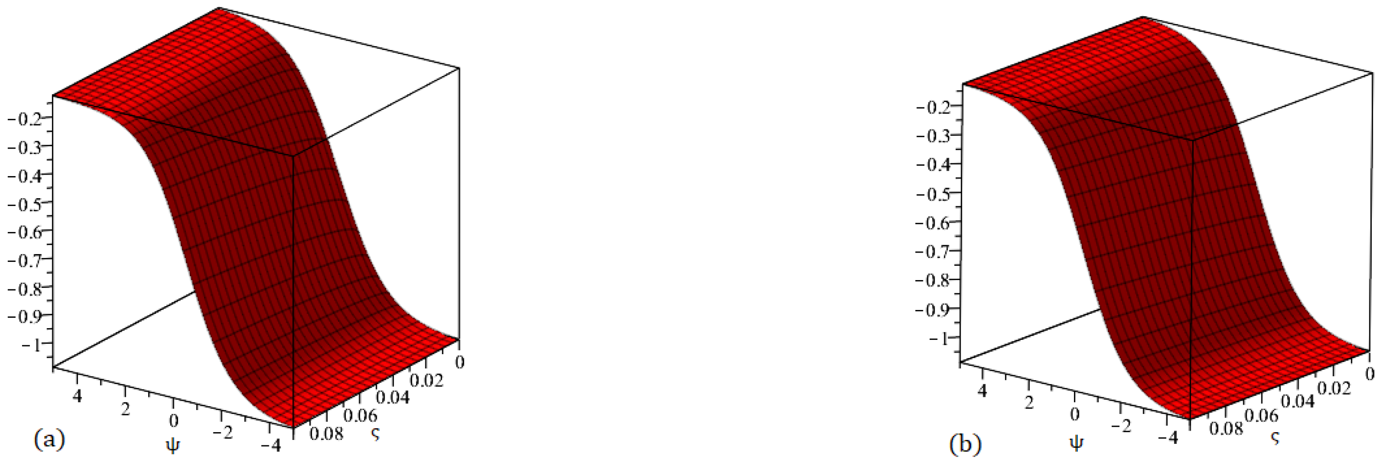
Figure 1.
Graph (a) demonstrating the accurate solution and (b) demonstrating our method solution for .
Figure 1.
Graph (a) demonstrating the accurate solution and (b) demonstrating our method solution for .
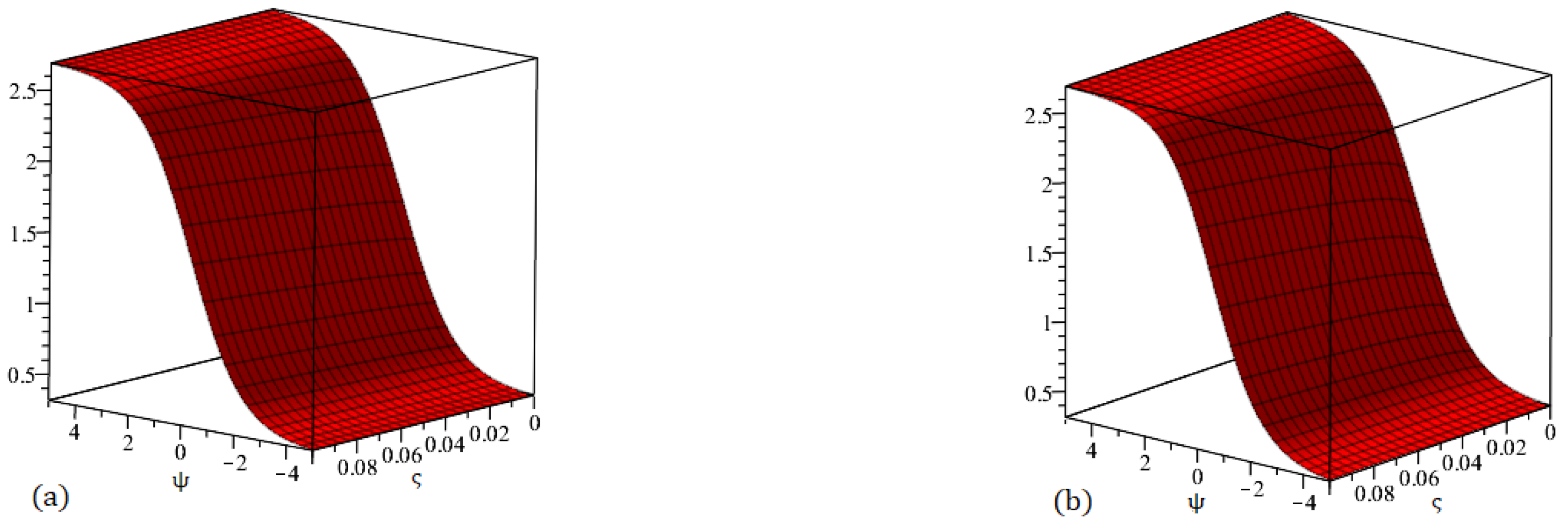
Figure 2.
Graph (a) demonstrating the accurate solution and (b) demonstrating our method solution for .
Figure 2.
Graph (a) demonstrating the accurate solution and (b) demonstrating our method solution for .
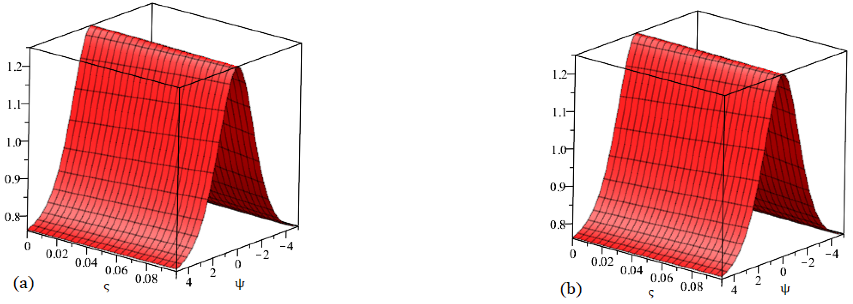
Figure 3.
Graph (a) demonstrating the accurate solution and (b) demonstrating our method solution for .
Figure 3.
Graph (a) demonstrating the accurate solution and (b) demonstrating our method solution for .
Figure 4.
Graphs demonstrating our method solution for at (a) and (b) .
Figure 4.
Graphs demonstrating our method solution for at (a) and (b) .
Figure 5.
Graphs demonstrating our method solution for at (a) and (b) .
Figure 5.
Graphs demonstrating our method solution for at (a) and (b) .
Figure 6.
Graphs demonstrating our method solution for at (a) and (b) .
Figure 6.
Graphs demonstrating our method solution for at (a) and (b) .
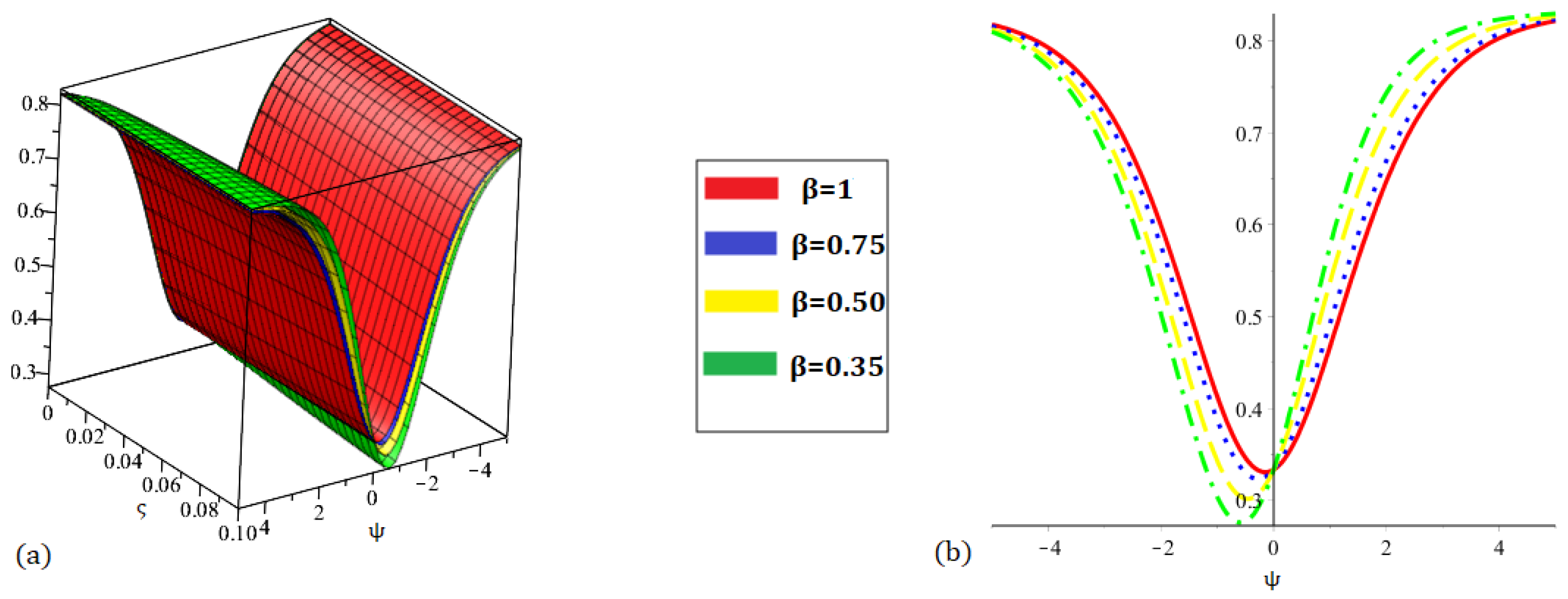
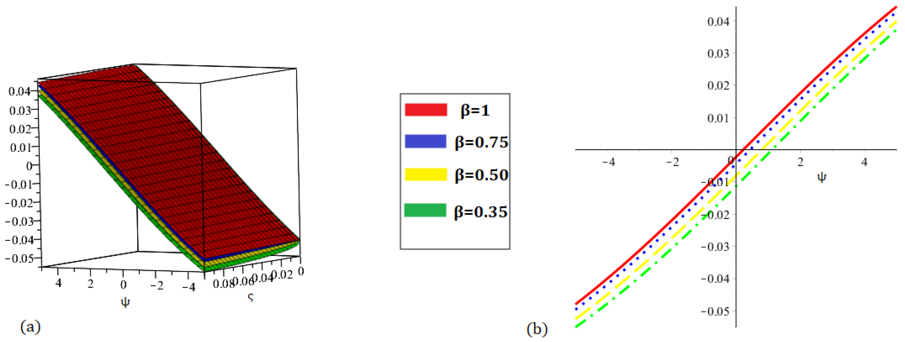
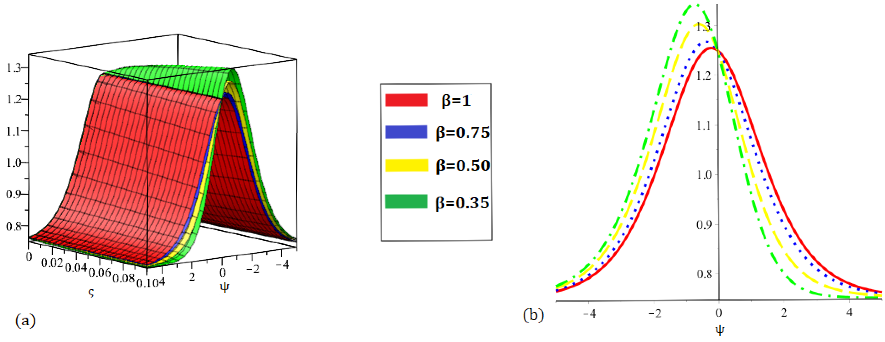
Figure 7.
Graph (a) demonstrating three-dimensional and (b) demonstrating two-dimensional nature of the proposed method result for at various fractional orders of .
Figure 7.
Graph (a) demonstrating three-dimensional and (b) demonstrating two-dimensional nature of the proposed method result for at various fractional orders of .
Figure 8.
Graph (a) demonstrating three-dimensional and (b) demonstrating two-dimensional nature of the proposed method result for at various fractional orders of .
Figure 8.
Graph (a) demonstrating three-dimensional and (b) demonstrating two-dimensional nature of the proposed method result for at various fractional orders of .
Figure 9.
Graph (a) demonstrating three-dimensional and (b) demonstrating two-dimensional nature of the proposed method result for at various fractional orders of .
Figure 9.
Graph (a) demonstrating three-dimensional and (b) demonstrating two-dimensional nature of the proposed method result for at various fractional orders of .
Figure 10.
Graph (a) demonstrating the accurate solution and (b) demonstrating our method solution for .
Figure 10.
Graph (a) demonstrating the accurate solution and (b) demonstrating our method solution for .
Figure 11.
Graph (a) demonstrating the accurate solution and (b) demonstrating our method solution for .
Figure 11.
Graph (a) demonstrating the accurate solution and (b) demonstrating our method solution for .
Figure 12.
Graphs demonstrating our method solution for at (a) and (b) .
Figure 12.
Graphs demonstrating our method solution for at (a) and (b) .
Figure 13.
Graphs demonstrating our method solution for at (a) and (b) .
Figure 13.
Graphs demonstrating our method solution for at (a) and (b) .
Figure 14.
Graph (a) demonstrating three-dimensional and (b) demonstrating two-dimensional nature of the proposed method result for at various fractional orders of .
Figure 14.
Graph (a) demonstrating three-dimensional and (b) demonstrating two-dimensional nature of the proposed method result for at various fractional orders of .
Figure 15.
Graph (a) demonstrating three-dimensional and (b) demonstrating two-dimensional nature of the proposed method result for at various fractional orders of .
Figure 15.
Graph (a) demonstrating three-dimensional and (b) demonstrating two-dimensional nature of the proposed method result for at various fractional orders of .
Table 1.
Numerical comparison between accurate and proposed method solution at different fractional orders for .
Table 1.
Numerical comparison between accurate and proposed method solution at different fractional orders for .
| | | | | |
|---|
| 0.0 | 0.4933335653 | 0.4933334681 | 0.4933334114 | 0.4933333783 | 0.4933333783 |
| 0.1 | 0.4933368309 | 0.4933364566 | 0.4933361820 | 0.4933359781 | 0.4933359781 |
| 0.2 | 0.4933440935 | 0.4933434422 | 0.4933429500 | 0.4933425755 | 0.4933425755 |
| 0.3 | 0.4933553470 | 0.4933544196 | 0.4933537101 | 0.4933531651 | 0.4933531652 |
| 0.4 | 0.4933705829 | 0.4933693797 | 0.4933684537 | 0.4933677388 | 0.4933677388 |
| 0.5 | 0.4933897886 | 0.4933883109 | 0.4933871689 | 0.4933862847 | 0.4933862846 |
| 0.6 | 0.4934129491 | 0.4934111977 | 0.4934098409 | 0.4934087881 | 0.4934087880 |
| 0.7 | 0.4934400458 | 0.4934380223 | 0.4934364515 | 0.4934352309 | 0.4934352308 |
| 0.8 | 0.4934710572 | 0.4934687632 | 0.4934669798 | 0.4934655923 | 0.4934655922 |
| 0.9 | 0.4935059587 | 0.4935033961 | 0.4935014015 | 0.4934998482 | 0.4934998481 |
| 1.0 | 0.4935447229 | 0.4935418936 | 0.4935396892 | 0.4935379714 | 0.4935379714 |
Table 2.
Numerical comparison between accurate and proposed method solutions at different fractional orders for .
Table 2.
Numerical comparison between accurate and proposed method solutions at different fractional orders for .
| | | | | |
|---|
| 0.0 | −3.0193627730 | −3.0195023340 | −3.0196119980 | −3.0196980000 | −3.0196980000 |
| 0.1 | −3.0173495930 | −3.0174891320 | −3.0175987790 | −3.0176847690 | −3.0176847690 |
| 0.2 | −3.0153369450 | −3.0154764300 | −3.0155860390 | −3.0156720000 | −3.0156720000 |
| 0.3 | −3.0133252270 | −3.0134646340 | −3.0135741820 | −3.0136600970 | −3.0136600970 |
| 0.4 | −3.0113148430 | −3.0114541430 | −3.0115636080 | −3.0116494600 | −3.0116494600 |
| 0.5 | −3.0093061930 | −3.0094453590 | −3.0095547200 | −3.0096404910 | −3.0096404900 |
| 0.6 | −3.0072996750 | −3.0074386780 | −3.0075479140 | −3.0076335870 | −3.0076335870 |
| 0.7 | −3.0052956880 | −3.0054345000 | −3.0055435890 | −3.0056291470 | −3.0056291470 |
| 0.8 | −3.0032946250 | −3.0034332200 | −3.0035421390 | −3.0036275680 | −3.0036275670 |
| 0.9 | −3.0012968810 | −3.0014352310 | −3.0015439600 | −3.0016292390 | −3.0016292400 |
| 1.0 | −2.9993028430 | −2.9994409220 | −2.9995494400 | −2.9996345550 | −2.9996345550 |
Table 3.
Numerical comparison between accurate and proposed method solutions at different fractional orders for .
Table 3.
Numerical comparison between accurate and proposed method solutions at different fractional orders for .
| | | | | |
|---|
| 0.0 | 1.5003165040 | 1.5002471850 | 1.5001927160 | 1.5001500000 | 1.5001500000 |
| 0.1 | 1.5013164270 | 1.5012471200 | 1.5011926600 | 1.5011499500 | 1.5011499490 |
| 0.2 | 1.5023160870 | 1.5022468060 | 1.5021923640 | 1.5021496690 | 1.5021496690 |
| 0.3 | 1.5033152840 | 1.5032460430 | 1.5031916310 | 1.5031489580 | 1.5031489590 |
| 0.4 | 1.5043138200 | 1.5042446310 | 1.5041902600 | 1.5041476190 | 1.5041476190 |
| 0.5 | 1.5053114930 | 1.5052423710 | 1.5051880530 | 1.5051454520 | 1.5051454520 |
| 0.6 | 1.5063081080 | 1.5062390670 | 1.5061848110 | 1.5061422580 | 1.5061422580 |
| 0.7 | 1.5073034660 | 1.5072345200 | 1.5071803370 | 1.5071378400 | 1.5071378410 |
| 0.8 | 1.5082973720 | 1.5082285340 | 1.5081744340 | 1.5081320030 | 1.5081320030 |
| 0.9 | 1.5092896290 | 1.5092209110 | 1.5091669070 | 1.5091245500 | 1.5091245500 |
| 1.0 | 1.5102800450 | 1.5102114610 | 1.5101575620 | 1.5101152870 | 1.5101152870 |
Table 4.
Numerical comparison between proposed method solution with accurate solution and fractional reduced differential transform method (FRDTM) for .
Table 4.
Numerical comparison between proposed method solution with accurate solution and fractional reduced differential transform method (FRDTM) for .
| | | | |
|---|
| | 0.0 | 0.493351 | 0.493333 | 0.493351 |
| | 0.25 | 0.493393 | 0.493345 | 0.493393 |
| 0.2 | 0.50 | 0.493460 | 0.493381 | 0.493460 |
| | 0.75 | 0.493552 | 0.493443 | 0.493552 |
| | 1.0 | 0.493667 | 0.493528 | 0.493667 |
| | 0.0 | 0.493405 | 0.493333 | 0.493405 |
| | 0.25 | 0.493477 | 0.493344 | 0.493477 |
| 0.4 | 0.50 | 0.493573 | 0.493380 | 0.493573 |
| | 0.75 | 0.493693 | 0.493440 | 0.493693 |
| | 1.0 | 0.493836 | 0.493525 | 0.493836 |
| | 0.0 | 0.493494 | 0.493333 | 0.493495 |
| | 0.25 | 0.493595 | 0.493343 | 0.493596 |
| 0.6 | 0.50 | 0.493720 | 0.493378 | 0.493721 |
| | 0.75 | 0.493868 | 0.493438 | 0.493868 |
| | 1.0 | 0.494038 | 0.493523 | 0.494038 |
Table 5.
Numerical comparison between proposed method solution with accurate solution and FRDTM for .
Table 5.
Numerical comparison between proposed method solution with accurate solution and FRDTM for .
| | | | |
|---|
| | 0.0 | −3.013961 | −3.019919 | −3.013960 |
| | 0.25 | −3.008937 | −3.014887 | −3.008936 |
| 0.2 | 0.50 | −3.003927 | −3.009862 | −3.003925 |
| | 0.75 | −2.998937 | −3.004849 | −2.998935 |
| | 1.0 | −2.993973 | −2.999856 | −2.993971 |
| | 0.0 | −3.007934 | −3.019839 | −3.007920 |
| | 0.25 | −3.002927 | −3.014807 | −3.002913 |
| 0.4 | 0.50 | −2.997942 | −3.009782 | −2.997927 |
| | 0.75 | −2.992984 | −3.004771 | −2.992969 |
| | 1.0 | −2.988058 | −2.999779 | −2.988045 |
| | 0.0 | −3.001928 | −3.019758 | −3.001880 |
| | 0.25 | −2.996948 | −3.014727 | −2.996899 |
| 0.6 | 0.50 | −2.991996 | −3.009703 | −2.991948 |
| | 0.75 | −2.987078 | −3.004693 | −2.987031 |
| | 1.0 | −2.982200 | −2.999702 | −2.982154 |
Table 6.
Numerical comparison between proposed method solution with accurate solution and FRDTM for .
Table 6.
Numerical comparison between proposed method solution with accurate solution and FRDTM for .
| | | | |
|---|
| | 0.0 | 1.502999 | 1.500039 | 1.503000 |
| | 0.25 | 1.505494 | 1.502539 | 1.505495 |
| 0.2 | 0.50 | 1.507983 | 1.505035 | 1.507983 |
| | 0.75 | 1.510461 | 1.507525 | 1.510462 |
| | 1.0 | 1.512927 | 1.510005 | 1.512928 |
| | 0.0 | 1.505993 | 1.500079 | 1.506000 |
| | 0.25 | 1.508479 | 1.502579 | 1.508383 |
| 0.4 | 0.50 | 1.510956 | 1.505075 | 1.510756 |
| | 0.75 | 1.513418 | 1.507564 | 1.513117 |
| | 1.0 | 1.515865 | 1.510043 | 1.515463 |
| | 0.0 | 1.508975 | 1.500111 | 1.509000 |
| | 0.25 | 1.511449 | 1.502619 | 1.511381 |
| 0.6 | 0.50 | 1.513909 | 1.505114 | 1.513749 |
| | 0.75 | 1.516352 | 1.507603 | 1.516100 |
| | 1.0 | 1.518774 | 1.510081 | 1.518433 |
Table 7.
Numerical comparison between proposed method solution and q-homotopy analysis transform method (q-HATM) for .
Table 7.
Numerical comparison between proposed method solution and q-homotopy analysis transform method (q-HATM) for .
| q−HATM | |
|---|
| −50 | 1.502999 | 1.000000 |
| −40 | 8.46214 | 1.000000 |
| −30 | 6.03700 | 2.000000 |
| −20 | 3.38628 | 1.600000 |
| −10 | 5.51964 | 2.500000 |
| 0 | 9.24074 | 1.300000 |
| 10 | 4.87746 | 5.500000 |
| 20 | 3.31997 | 1.800000 |
| 30 | 5.86792 | 2.000000 |
| 40 | 8.21664 | 0.00000000 |
| 50 | 1.11710 | 0.00000000 |
Table 8.
Numerical comparison between proposed method solution and q-homotopy analysis transform method (q-HATM) for .
Table 8.
Numerical comparison between proposed method solution and q-homotopy analysis transform method (q-HATM) for .
| q−HATM | |
|---|
| −50 | 1.15064 | 4.15000 |
| −40 | 8.46214 | 2.838000 |
| −30 | 6.03701 | 2.637000 |
| −20 | 3.38628 | 1.733000 |
| −10 | 5.51964 | 4.610000 |
| 0 | 9.24074 | 1.400000 |
| 10 | 4.87746 | 4.600000 |
| 20 | 3.31998 | 1.800000 |
| 30 | 5.86792 | 2.000000 |
| 40 | 8.21664 | 0.00000000 |
| 50 | 1.11710 | 0.00000000 |


