Time-Fractional Evolution of Quantum Dense Coding Under Amplitude Damping Noise

Abstract

In this paper, we investigate the memory effects introduced by the time-fractional Schrödinger equation proposed by Naber on quantum entanglement and quantum dense coding under amplitude damping noise. Two formulations are analyzed: one with fractional operations applied to the imaginary unit and one without. Numerical results show that the formulation without fractional operations on the imaginary unit may be more suitable for describing non-Markovian (power-law) behavior in dissipative environments. This finding provides a more physically meaningful interpretation of the memory effects in time-fractional quantum dynamics and indirectly addresses fundamental concerns regarding the violation of unitarity and probability conservation in such frameworks. Our work offers a new perspective for the application of fractional quantum mechanics to realistic open quantum systems and shows promise in supporting the theoretical modeling of decoherence and information degradation.

1. Introduction

The study of physical systems has traditionally been grounded in well-established mathematical frameworks and physical principles [1]. In classical mechanics, time is generally treated as isotropic and independent of spatial variables, while space is assumed to be continuous and homogeneous. These assumptions, in conjunction with integer-order calculus, have enabled a robust description of deterministic phenomena. In quantum mechanics, the Schrödinger equation serves as a foundational equation for describing the evolution of quantum states in both time and space [2,3]. Its formulation relies on integer-order derivatives, implicitly assuming smooth and uniform temporal evolution. However, growing evidence suggests that many physical systems, especially at microscopic and statistical levels, deviate from these classical assumptions [4,5,6]. Phenomena such as long-range memory, fractal geometries, and non-Markovian dynamics challenge the adequacy of integer-order models. These complexities reveal limitations in traditional calculus when applied to systems exhibiting history dependence and anomalous transport. In response, fractional calculus, which generalizes differentiation and integration to non-integer orders, has emerged as a powerful mathematical framework for overcoming the limitations of classical integer-order models [7,8,9,10].

One notable application of fractional calculus in quantum theory is the time-fractional Schrödinger equation (TFSE), which was proposed by Naber to describe non-Markovian quantum evolution [11]. His approach involves mapping the time-fractional diffusion equation into a Schrödinger-like form, analogous to the classical correspondence between the diffusion equation and the standard Schrödinger equation. It is important to emphasize that the construction of this equation does not originate from the first principles of quantum mechanics. Instead, it is based on a substitution method, wherein the first-order time derivative in the conventional Schrödinger equation is formally replaced by a fractional-order Caputo derivative. Although this heuristic approach is mathematically self-consistent, it lacks a rigorous foundation in quantum theory, and its physical interpretation remains a subject of ongoing scrutiny. In terms of different treatments to the imaginary unit i, Naber constructed two types of TFSE. The choice and role of the imaginary unit are non-trivial: it is essential for preserving quantum coherence, enabling interference, and ensuring the probabilistic interpretation of the wave function. This distinguishes the TFSE from fractional diffusion equations, which lack such phase-related structure. Therefore, determining the appropriate formulation of the imaginary unit in the TFSE is a critical consideration [11,12,13,14]. In the past two decades, the TFSE has found applications in diverse areas such as optics [15], free-particle dynamics [11], and optical solitons [16], with promising results also reported in recent studies [17,18,19,20]. However, the introduction of the Caputo derivative causes a deviation from the framework of standard quantum mechanics. Specifically, it breaks unitary time evolution and violates probability conservation. This observation prompts us to reflect on whether it is appropriate to employ this type of equation to study non-Markovian dynamics in dissipative quantum systems, and whether such an approach could offer a plausible explanation for these two phenomena. Given the limited attention this framework has received in the context of quantum communication, we aim to explore its potential further by analyzing the behavior of quantum dense coding under amplitude damping noise. This investigation serves to assess the TFSE’s capacity to model dissipation and memory effects in quantum information processes.

Over the past decade, there has been significant advancement in understanding non-Markovian dynamics, where memory effects allow lost information to flow back into the system, potentially restoring coherence and entanglement [21,22,23]. For instance, in non-Markovian dissipative environments, entangled states may periodically decay and revive. However, due to the mathematical complexity of non-Markovian systems and the difficulty of solving the corresponding dynamical equations, the development of accurate and tractable models remains challenging [24,25]. This limitation continues to hinder the practical application of non-Markovian environments in real-world quantum communication systems. In this context, the time-fractional Schrödinger equation offers a promising alternative framework for describing non-Markovian dynamics [11]. Here, the order of the fractional time derivative serves as a tunable parameter that directly characterizes the strength of memory effects, enabling a more straightforward and flexible modeling approach. Unlike conventional methods, the TFSE-based framework does not require detailed modeling of environmental structure, time delays, or high-dimensional state spaces. As such, it presents a valuable and simplified tool for exploring the dynamics and practical applications of non-Markovian quantum systems.

The time-fractional Schrödinger equation is employed in this work as a phenomenological framework to model non-Markovian behavior. Its effectiveness lies in the capacity of fractional-order derivatives to mathematically characterize memory effects, without implying any alteration of the foundational principles of quantum mechanics. We utilize the time-fractional Schrödinger equation to investigate quantum dense coding under amplitude damping noise. The shared entangled state between the sender Alice and the receiver Bob is a composite state formed by the linear superposition of two Bell states, with the preparation of this composite state being accomplished by a third party, Charlie. When Charlie sends the particles to Alice and Bob, they experience amplitude damping noise (AD) with memory effects and identical noise strength. This noise can be physically modeled using the double Jaynes–Cummings (J-C) model. That is to say, the time-fractional Schrödinger equation is applied solely to describe the evolution of the shared quantum state during its transmission through the noisy channel. Our findings demonstrate that the TFSE without fractional operations involving the imaginary unit provides a more suitable framework for describing non-Markovian dynamics in dissipative quantum systems. The memory effects inherent in the TFSE significantly enhance the robustness of entangled states against environmental interference, even suppressing entanglement sudden death (ESD). Furthermore, we establish that stronger memory effects correlate with higher dense coding capacity. This work advances the understanding of the TFSE and presents a novel approach for its application in quantum information science.

This paper is organized as follows. In Section 2, we provide an overview of the time-fractional Schrödinger equation, quantum dense coding, and the double Jaynes–Cummings model as discussed in this work. Then, in Section 3, we study the quantum dense coding using the time-fractional Schrödinger equation. Finally, the discussions and conclusions are summarized in Section 4.

2. Overview of Key Concepts

In this section, we review the time-fractional Schrödinger equation proposed by Naber in Section 2.1, quantum dense coding in Section 2.2 and the double Jaynes–Cummings model in Section 2.3.

2.1. Time-Fractional Schrödinger Equation and Its Memory

The TFSE was first introduced by Naber, motivated by the development of the time-fractional diffusion equation. In his formulation, the first-order time derivative in the Schrödinger equation is formally replaced by a fractional-order derivative. However, unlike the diffusion equation, the Schrödinger equation involves the imaginary unit, which presents additional challenges in generalizing it to fractional time dynamics. To address this, Naber proposed two distinct forms of the TFSE, based on different treatments of the imaginary unit in the fractional derivative operator, which can be expressed as

$$i\hslash T_c^{\alpha -1}{\displaystyle \frac{{\partial }^{\alpha }}{\partial t}}{\psi }_{\alpha }(\overrightarrow{r},t)=\widehat{H}{\psi }_{\alpha }(\overrightarrow{r},t).$$

(1)

$$i^{\alpha }\hslash T_c^{\alpha -1}{\displaystyle \frac{{\partial }^{\alpha }}{\partial t}}{\psi }_{\alpha }(\overrightarrow{r},t)=\widehat{H}{\psi }_{\alpha }(\overrightarrow{r},t),$$

(2)

where ℏ is the reduced Planck constant, ${\psi }_{\alpha }(\overrightarrow{r},t)$ is the wave function, i is the imaginary unit and $i=\sqrt{-1}$. $T_c$ is an arbitrary time constant, which is used to replace the Planck time $T_p$ [26]. ${\displaystyle \frac{{\partial }^{\alpha }}{\partial t}}$ is the Caputo fractional derivative of order $\alpha$ defined by

$${\displaystyle \frac{{\partial }^{\alpha }}{\partial t}}f\left(t\right)={}_0{}^{c}D_t^{\alpha }f\left(t\right)={\displaystyle \frac{1}{\mathsf{\Gamma }(1-\alpha )}}\underset{0}{\overset{t}{\int }}{\displaystyle \frac{f^{\prime }\left(\tau \right)}{{(t-\tau )}^{\alpha }}}d\tau (0<\alpha \le 1),$$

(3)

where $\mathsf{\Gamma }(1-\alpha )$ is the Gamma function and $f^{\prime }\left(\tau \right)$ is the first-order time derivative. The memory effects inherent in the TFSE are characterized by the order $\alpha$ of the fractional derivative. To further elucidate the origin of this memory, we rewrite Equation (3) as

$$\begin{array}{c}{\displaystyle \frac{{\partial }^{\alpha }}{\partial t}}f\left(t\right)={}_0{}^{c}D_t^{\alpha }f\left(t\right)={\displaystyle \frac{1}{\mathsf{\Gamma }(1-\alpha )}}\underset{0}{\overset{t}{\int }}{(t-\tau )}^{(1-\alpha )-1}{f}^{\prime }\left(\tau \right)d\tau \hfill \\ =r\left(t\right)\ast f^{\prime }\left(\tau \right)(0<\alpha \le 1)\hfill \end{array}$$

(4)

where $r\left(t\right)={\displaystyle \frac{1}{\mathsf{\Gamma }(1-\alpha )}}{t}^{-\alpha }$, and ∗ represents a convolution operation. Clearly, the Caputo fractional derivative is defined through fractional integration. As shown in Equation (4), evaluating a Caputo derivative of order $\alpha$ ($0<\alpha \le 1$) involves first computing the ordinary derivative $f^{\prime }\left(t\right)$, followed by a fractional integral of order $1-\alpha$. Thus, the Caputo fractional derivative can be interpreted as a weighted integral of the first derivative $f^{\prime }\left(t\right)$, where the weight decays as a power law determined by $\alpha$. The memory strength encoded in the kernel $r\left(t\right)$ decreases with increasing $\alpha$, indicating that the system “forgets” more quickly. Especially, when $\alpha \to 1$, $r\left(t\right)$ turns into a unit impulse function $\delta \left(t\right)$, and TFSE loses memory and becomes the standard Schrödinger equation. For $\alpha \to 0$, $r\left(t\right)$ becomes unit step function, and TFSE has full memory. To better understand the role of the TFSE in describing non-Markovian quantum dynamics, it is instructive to perform a systematic comparison with established theoretical frameworks, such as the Nakajima–Zwanzig (NZ) projection operator formalism and generalized master equations (GMEs) based on memory kernels. From the perspective of theoretical foundation, the NZ method and GME originate from the Liouville-von Neumann equation of the total system-plus-environment and are derived rigorously using projection operator techniques. In this framework, memory effects naturally arise from the microscopic interactions between the system and its environment. In contrast, the TFSE introduces memory effects phenomenologically by replacing the first-order time derivative in the standard Schrödinger equation with a fractional-order derivative, leading to a power-law memory kernel. This substitution is not derived from first principles but provides a mathematically tractable means to incorporate long-range memory effects. Structurally, the TFSE features a fixed power-law memory kernel of the form, capturing long-time correlations via convolution integrals. In comparison, the memory kernel in the NZ formalism depends on the spectral density of the environment and can exhibit richer behavior, including exponential decay, oscillations, or structured noise. The TFSE, due to its compact form, is particularly suitable for modeling systems with algebraically decaying memory, while the NZ approach, although more involved, offers stronger physical interpretability and can be tailored to specific open-system models. Therefore, TFSE may be viewed as a phenomenological approximation to the more rigorous NZ and GME frameworks, especially in scenarios where the memory follows a power-law distribution and detailed information about the environment is unavailable. Previous studies have shown that, at the specific fractional order $\alpha =0.5$, the TFSE is isospectral to a comb model [27]. Both Equations (1) and (2) violate the probability conservation law for $0<\alpha <1$. The total probability for Equation (1) will be decay to zero [28], while that for Equation (2) will be greater than one [11]. Clearly, for dissipative systems, Equation (1) offers a more intuitive interpretation.

2.2. Quantum Dense Coding

Quantum dense coding is a quantum communication protocol that leverages the properties of quantum entanglement to achieve efficient encoding of information in bit transmission. It allows the sender to transmit two bits of classical information by sending just one quantum bit when they share entangled quantum bits. During the preparation phase, the sender (Alice) and the receiver (Bob) share a pair of entangled quantum bits. In the encoding phase, Alice performs operations on her quantum bit based on the two classical bits she wants to send. For example, if she wants to send “00,” she performs no operation; if she wants to send “01,” she applies an X gate to her quantum bit. In the transmission phase, Alice sends her quantum bit to Bob. During the decoding phase, Bob measures the received quantum bit and decodes the two classical bits of information sent by Alice based on the measurement results. Compared to traditional communication methods, quantum dense coding enhances communication efficiency by allowing the transmission of two classical bits with the sending of just one quantum bit. In this work, as illustrated in Figure 1, the entangled quantum state is initially prepared by a third party (Charlie), and then transmitted to the sender (Alice) and the receiver (Bob) via quantum channels. During this transmission process, the entangled state is affected by amplitude damping noise with memory effects and identical noise strength. In this scenario, we describe the evolution using the time-fractional Schrödinger equation with Caputo fractional derivative, which is known to effectively model such non-Markovian behavior. Considering that environmental interference can lead to the decoherence of quantum entanglement, we need to optimize the channel to suppress noise. By utilizing mutually orthogonal unitary encoding operations, we can mitigate the impact of noise on the system, thereby achieving optimal dense coding capacity. Ultimately, the unitary encoding capacity over a quantum noisy channel can be expressed as follows

$$C=S\left(\overline{\rho }\right)-S\left(\rho \right)$$

(5)

where $\rho$ is a shared entangled state, $S\left(\rho \right)$ is the von Neumann entropy and $S\left(\rho \right)=-tr(\rho log\rho )=-\sum K_{i}log{K}_i$, $K_i$ are the eigenvalues of the density matrix $\rho$. $\overline{\rho }$ represents the average density matrix of the signal state set, which can be expressed as

$$\overline{\rho }={\displaystyle \frac{1}{4}}\sum _0^3(U_i\otimes I)\rho (U_i^{†}\otimes I)$$

(6)

where ⊗ denotes the tensor product. $U_i\otimes I$ represents the application of the unitary operator $U_i$ on the first qubit and the identity operation I on the second qubit. $U_i$ is a series of mutually orthogonal unitary transformations in the dense coding protocol of a qubit system, $U_i^{†}$ is the complex conjugate transpose of $U_i$. This paper mainly discusses a two-qubit system, which can be represented as follows

$$\begin{array}{c}{U}_0=\left(\begin{array}{cc}1& 0\\ 0& 1\end{array}\right),U_1=\left(\begin{array}{cc}0& 1\\ 1& 0\end{array}\right),\hfill \\ U_2=\left(\begin{array}{cc}1& 0\\ 0& -1\end{array}\right),U_3=\left(\begin{array}{cc}0& 1\\ -1& 0\end{array}\right).\hfill \end{array}$$

(7)

The advantage of the quantum dense coding protocol is reflected in the system capacity of two bits $1<C<2$. If the dense coding capacity is less than 1, then quantum dense coding loses its advantage and may even result in performance inferior to that of classical information transmission.

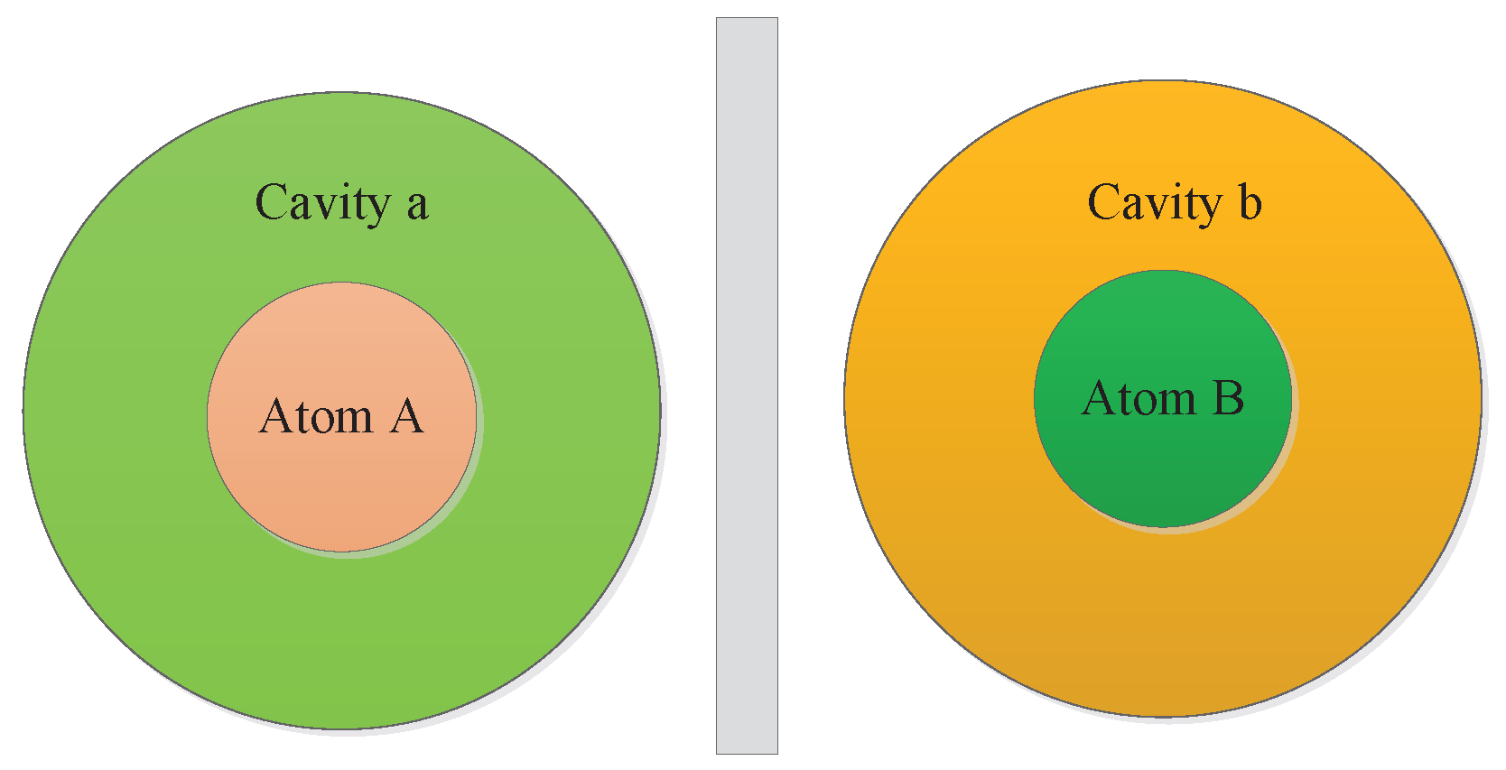
2.3. Double Jaynes–Cummings Model

In order to simulate the dynamical evolution of a shared entangled state in an amplitude damping noise environment, we use the double Jaynes–Cummings model. As shown in Figure 2, this model consists of two two-level atoms. Each atom is situated in a perfect single-mode nearly resonant cavity and interacts with its initially unexcited cavity mode, while each atom is completely isolated from the other atom and the cavity. The Hamiltonian of the double Jaynes–Cummings model can be expressed as

$$\begin{array}{c}H={\omega }_A{\sigma }_{+}^A{\sigma }_{-}^A+{\omega }_B{\sigma }_{+}^B{\sigma }_{-}^B+\lambda (a{\sigma }_{+}^A+a^{†}{\sigma }_{-}^A)\hfill \\ +\lambda (b{\sigma }_{+}^B+b^{†}{\sigma }_{-}^B)+{\omega }_a{a}^{†}a+{\omega }_b{b}^{†}b.\hfill \end{array}$$

(8)

$\lambda$ denotes the coupling coefficient between the two subsystems, and ${\sigma }_{+}$ and ${\sigma }_{-}$ are the raising and lowering operators of the two-level system, respectively. ${\sigma }_{+}$ represents a transition from the ground state to the excited state, typically corresponding to the absorption of a photon. Conversely, ${\sigma }_{-}$ describes a transition from the excited state to the ground state, corresponding to the emission of a photon. $a^{†}$ and a are the creation and annihilation operators of a single-mode cavity, respectively. $a^{†}$ creates a photon in the cavity mode, increasing the photon number state $\left|n\right.〉$ to $\left|n+1\right.〉$. Conversely, a annihilates a photon, reducing the photon number state from $\left|n\right.〉$ to $\left|n-1\right.〉$. These operators collectively form the foundational components of the Jaynes–Cummings model, which captures the essential dynamics of the interaction between a quantized field and a two-level atom. It is important to note that the photon lost to the cavity does not vanish, and the photon can return to the atom over time. Considering the characteristics of amplitude damping noise, which primarily models energy dissipation in quantum systems, we only need to focus on the stage where the photon is lost to the cavity.

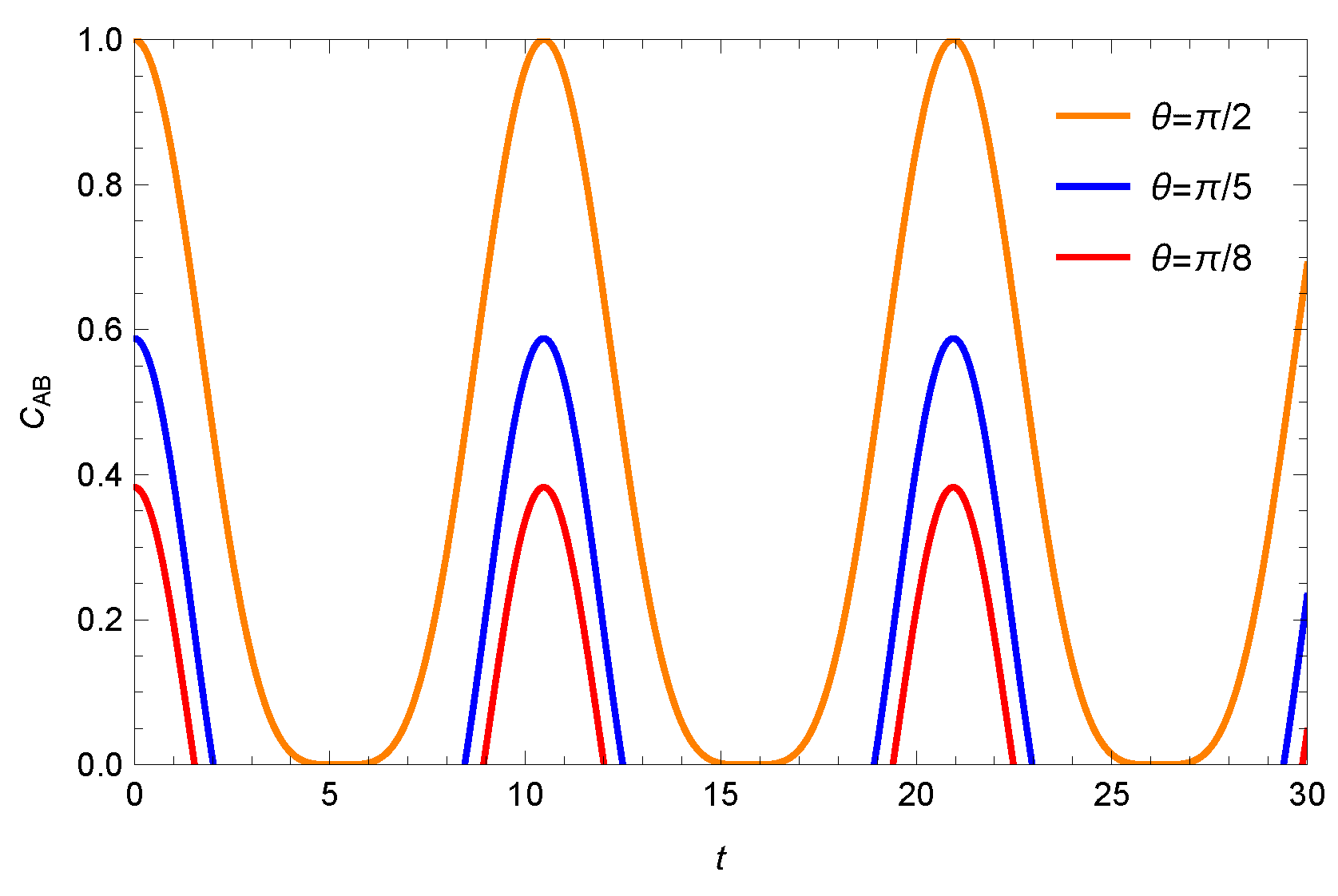
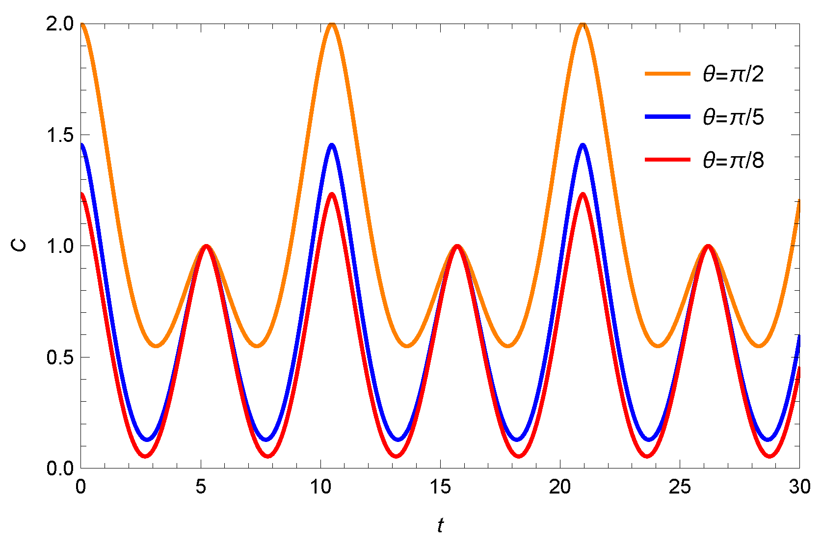
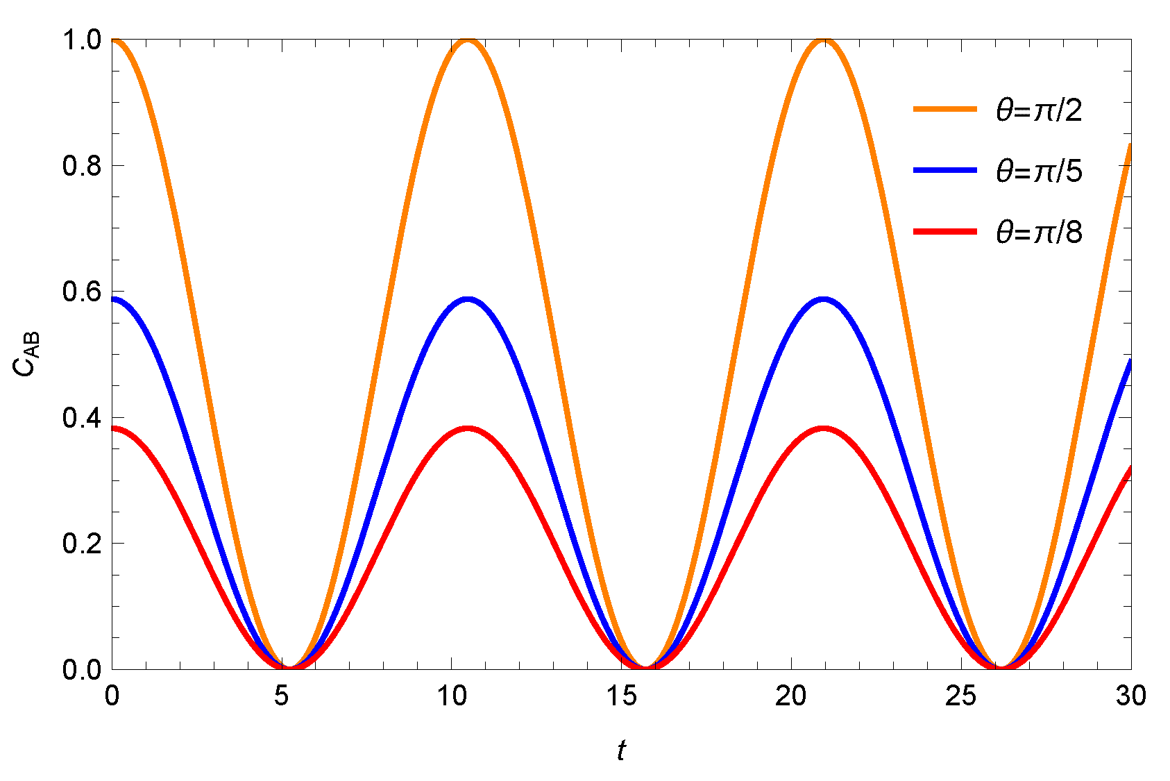
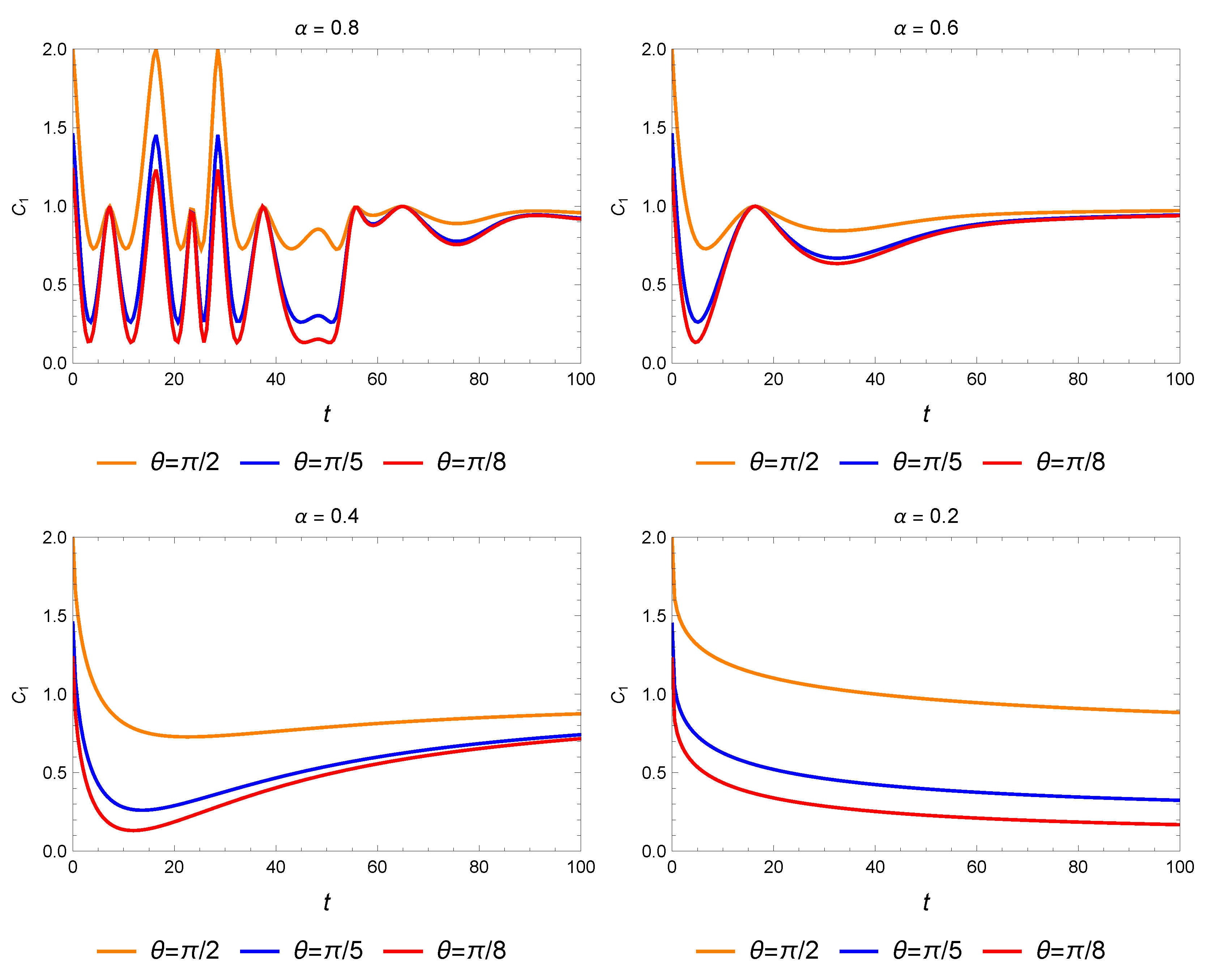
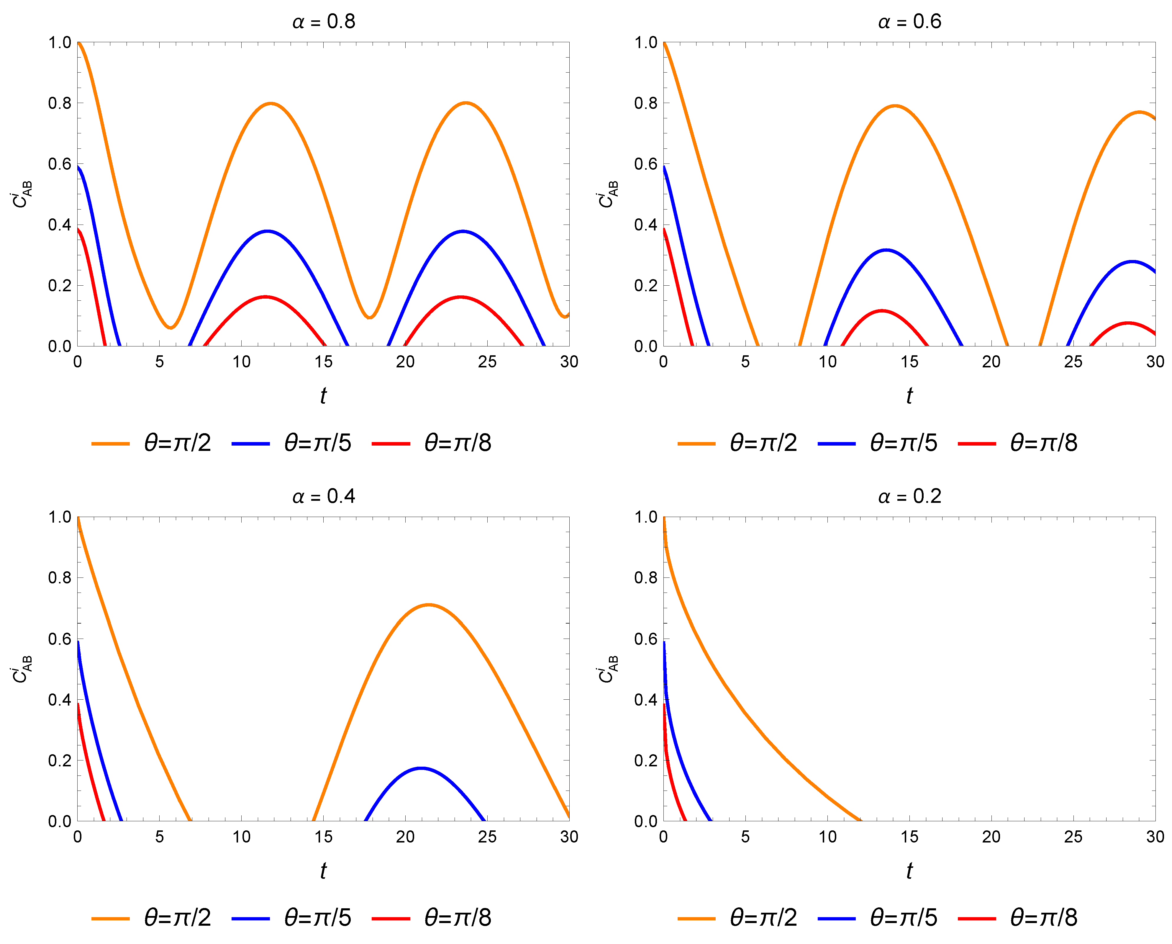
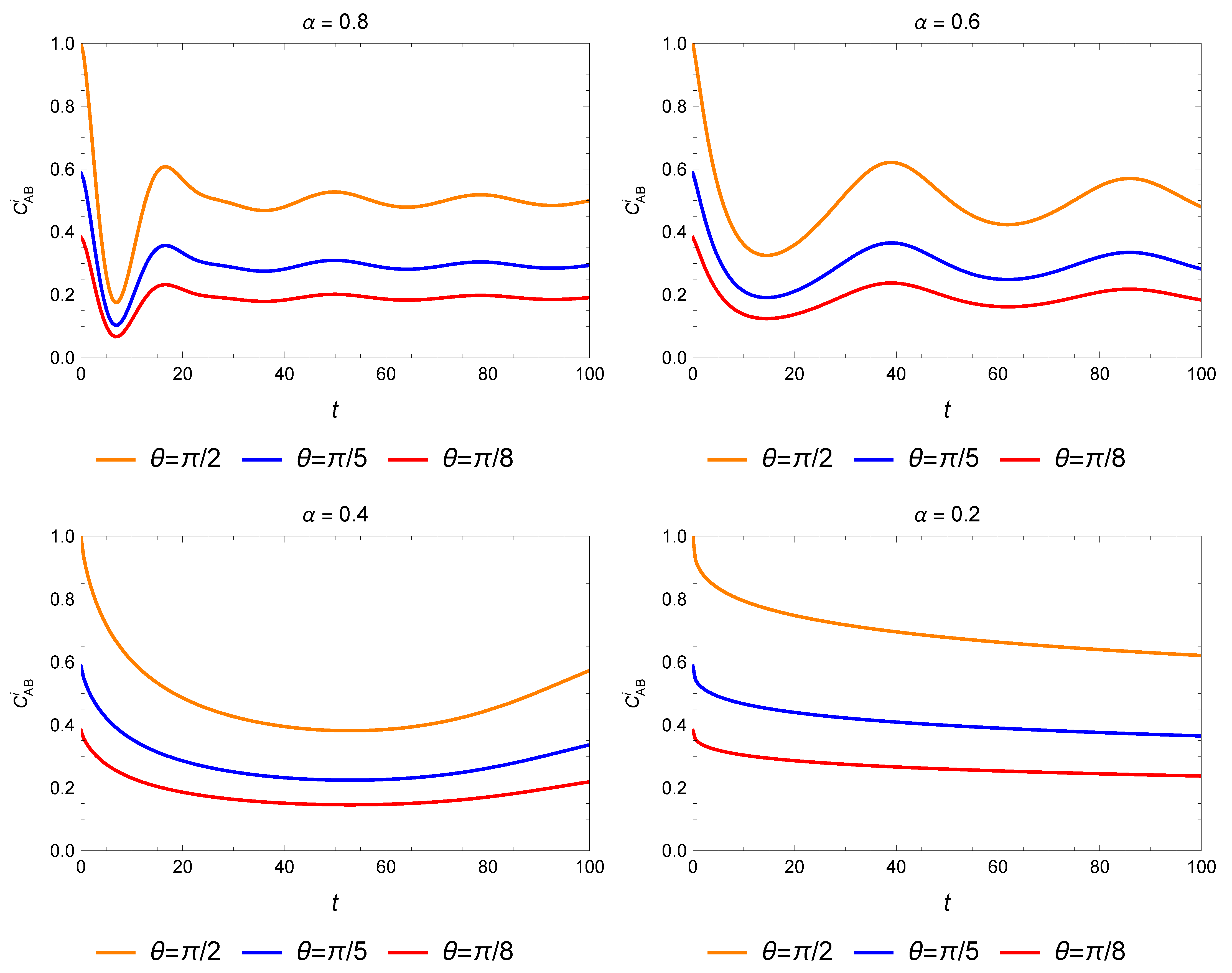
3. Time Fractional Evolution of Quantum Dense Coding

In this section, we explore the time-fractional evolution of quantum dense coding. The strengths and limitations of Equations (1) and (2) have been extensively analyzed, revealing that the suitability of each equation depends on the specific application. To provide a comprehensive understanding, we employ both equations in our study of quantum dense coding. Without loss of generality, supposing that $\hslash T_c^{\alpha -1}=1$ [26]. From the general analysis of a fractional differential linear system [29], the solution of Equation (1) takes the form,

$$\begin{array}{c}{\psi }_{\alpha }(\overrightarrow{r},t)=c_1{E}_{\alpha }(-i{k}_1{t}^{\alpha })u_1+c_2{E}_{\alpha }(-i{k}_2{t}^{\alpha })u_2\hfill \\ +....+c_n{E}_{\alpha }(-i{k}_n{t}^{\alpha })u_n,\hfill \end{array}$$

(9)

Similarly, the solution of Equation (2) can be expressed

$$\begin{array}{c}{\psi }_{\alpha }(\overrightarrow{r},t)=c_1{E}_{\alpha }\left(i^{-\alpha }{k}_1{t}^{\alpha }\right)u_1+c_2{E}_{\alpha }\left(i^{-\alpha }{k}_2{t}^{\alpha }\right)u_2\hfill \\ +....+c_n{E}_{\alpha }\left(i^{-\alpha }{k}_n{t}^{\alpha }\right)u_n,\hfill \end{array}$$

(10)

where $c_i$ are arbitrary constants, and $k_i$ and $u_i(i=1,2,\dots ,n)$ are the eigenvalues and the corresponding eigenvectors of the matrix $\widehat{H}$. The expression $E_{\beta }\left(k_i{t}^{\beta }\right)$ denotes the Mittag–Leffler function, which is relevant for their connection with fractional calculus, and is defined as

$$E_{\beta }\left(z\right)=\sum _{j=0}^{\infty }{\displaystyle \frac{z^j}{\mathsf{\Gamma }(\beta j+1)}},\beta >0,z\in C.$$

(11)

In order to ensure the reliability of the conclusions, we employ a linear combination of two Bell states as the shared entangled states for quantum dense coding, represented as follows

$${\psi }_{AB}=cos{\displaystyle \frac{\theta }{2}}\left|0_A{0}_B\right.〉+sin{\displaystyle \frac{\theta }{2}}\left|1_A{1}_B\right.〉,$$

(12)

$${\psi }_{AB}=cos{\displaystyle \frac{\theta }{2}}\left|0_A{1}_B\right.〉+sin{\displaystyle \frac{\theta }{2}}\left|1_A{0}_B\right.〉,$$

(13)

where $\left|0\right.〉$, $\left|1\right.〉$ represent the ground state and excited state, respectively. The subscripts A and B indicate the A and B quantum systema, respectively. Specifically, the shared entangled state becomes a maximally entangled state when $\theta =\pi /2$.

3.1. The Imaginary Unit Has No Operation

This section adopts the model given by Equation (1), in which the conventional imaginary unit is preserved, and only the time derivative is fractionalized. To simulate the situation of amplitude damping noise, we assume that both cavities are prepared initially in the vacuum state $\left|00\right.〉$, and the two atoms are in a pure entangled state specified Equation (12). The initial state for the total system is given by

$$\begin{array}{c}\left|{\psi }_0\right.〉=(cos{\displaystyle \frac{\theta }{2}}\left|0_A{0}_B\right.〉+sin{\displaystyle \frac{\theta }{2}}\left|1_A{1}_B\right.〉)\otimes \left|00\right.〉\hfill \\ =cos{\displaystyle \frac{\theta }{2}}\left|0_A{0}_{B}00\right.〉+sin{\displaystyle \frac{\theta }{2}}\left|1_A{1}_{B}00\right.〉\hfill \end{array}$$

(14)

Under the influence of amplitude damping noise, the state change due to energy dissipation is as follows

$$\begin{array}{c}\left|0_A{0}_{B}00\right.〉\to \left|0_A{0}_{B}00\right.〉,\hfill \\ \left|1_A{1}_{B}00\right.〉\to \left|1_A{0}_{B}01\right.〉\to \left|0_A{0}_{B}11\right.〉,\hfill \\ \left|1_A{1}_{B}00\right.〉\to \left|0_A{1}_{B}10\right.〉\to \left|0_A{0}_{B}11\right.〉.\hfill \end{array}$$

(15)

Therefore, the system state at time t can be expressed as

$$\begin{array}{c}\left|{\psi }_t\right.〉=x_1\left|0_A{0}_{B}11\right.〉+x_2\left|0_A{1}_{B}10\right.〉\hfill \\ +x_3\left|1_A{0}_{B}01\right.〉+x_4\left|1_A{1}_{B}00\right.〉+x_5\left|0_A{0}_{B}00\right.〉\hfill \end{array}$$

(16)

Using basis $\{\left|0_A{0}_{B}11\right.〉, \left|0_A{1}_{B}10\right.〉, \left|1_A{0}_{B}01\right.〉, \left|1_A{1}_{B}00\right.〉\}$, then assume ${\omega }_A={\omega }_B={\omega }_a={\omega }_b$. In the interaction picture, the Hamiltonian can be expressed as

$$H_I=\left(\begin{array}{cccc}0& \lambda & \lambda & 0\\ \lambda & 0& 0& \lambda \\ \lambda & 0& 0& \lambda \\ 0& \lambda & \lambda & 0\end{array}\right)$$

(17)

The corresponding eigenvalues and eigenvectors of $H_I$ are simply calculated as

$$\begin{array}{c}{k}_1=0,u_1=\left(\begin{array}{c}0\\ -1\\ 1\\ 0\end{array}\right).k_2=0,u_2=\left(\begin{array}{c}-1\\ 0\\ 0\\ 1\end{array}\right).\hfill \\ k_3=-2\lambda ,u_3=\left(\begin{array}{c}1\\ -1\\ -1\\ 1\end{array}\right).k_4=2\lambda ,u_4=\left(\begin{array}{c}1\\ 1\\ 1\\ 1\end{array}\right).\hfill \end{array}$$

(18)

From Equations (1), (9), and (18), the final entangled state can be expressed as

$$\left|\psi \left(t\right)\right.〉=c_1\left(\begin{array}{c}0\\ -1\\ 1\\ 0\end{array}\right)+c_2\left(\begin{array}{c}-1\\ 0\\ 0\\ 1\end{array}\right)+c_3\left(\begin{array}{c}1\\ -1\\ -1\\ 1\end{array}\right)E_{\alpha }\left(2\lambda i{t}^{\alpha }\right)+c_4\left(\begin{array}{c}0\\ -1\\ 0\\ 1\end{array}\right)E_{\alpha }(-2\lambda i{t}^{\alpha }),$$

(19)

The constants $c_1$, $c_2$, $c_3$ and $c_4$ can be obtained by Equation (14)

$$\begin{array}{c}{c}_1=0,c_2={\displaystyle \frac{1}{2}}cos{\displaystyle \frac{\theta }{2}},\hfill \\ c_3=c_4={\displaystyle \frac{1}{4}}cos{\displaystyle \frac{\theta }{2}},\hfill \end{array}$$

(20)

Therefore,

$$\begin{array}{c}{x}_1=-{\displaystyle \frac{1}{2}}cos{\displaystyle \frac{\theta }{2}}+{\displaystyle \frac{1}{4}}cos{\displaystyle \frac{\theta }{2}}[E_{\alpha }\left(2\lambda i{t}^{\alpha }\right)+E_{\alpha }(-2\lambda i{t}^{\alpha })]\hfill \\ x_2=x_3={\displaystyle \frac{1}{4}}cos{\displaystyle \frac{\theta }{2}}[E_{\alpha }(-2\lambda i{t}^{\alpha })-E_{\alpha }\left(2\lambda i{t}^{\alpha }\right)]\hfill \\ x_4={\displaystyle \frac{1}{2}}cos{\displaystyle \frac{\theta }{2}}+{\displaystyle \frac{1}{4}}cos{\displaystyle \frac{\theta }{2}}[E_{\alpha }\left(2\lambda i{t}^{\alpha }\right)+E_{\alpha }(-2\lambda i{t}^{\alpha })]\hfill \\ x_5=sin{\displaystyle \frac{\theta }{2}}\hfill \end{array}.$$

(21)

The information about the entanglement of two atoms is contained in the reduced density matrix ${\rho }_{AB}$, which can be obtained from Equation (16). The explicit $4\times 4$ matrix written in the basis $\{\left|00\right.〉, \left|01\right.〉, \left|10\right.〉, \left|11\right.〉\}$ is given by

$${\rho }_{AB}={\displaystyle \frac{1}{N}}\left(\begin{array}{cccc}a& 0& 0& b\\ 0& c& 0& 0\\ 0& 0& c& 0\\ b^{*}& 0& 0& d\end{array}\right),$$

(22)

where $N={\displaystyle \frac{1}{4}}{cos}^2{\displaystyle \frac{\theta }{2}}({\left|E_{\alpha }\left(2\lambda i{t}^{\alpha }\right)\right|}^2+{\left|E_{\alpha }(-2\lambda i{t}^{\alpha })\right|}^2+2)+{sin}^2{\displaystyle \frac{\theta }{2}}$ is the normalization factor, and the other parameters are as follows

$$\begin{array}{c}a={sin}^2{\displaystyle \frac{\theta }{2}}+{\displaystyle \frac{1}{16}}{cos}^2{\displaystyle \frac{\theta }{2}}{\left|E_{\alpha }\left(2\lambda i{t}^{\alpha }\right)+E_{\alpha }(-2\lambda i{t}^{\alpha })-2\right|}^2\hfill \\ b={\displaystyle \frac{1}{4}}\left|cos{\displaystyle \frac{\theta }{2}}\right|\left|sin{\displaystyle \frac{\theta }{2}}\right|\left|E_{\alpha }\left(2\lambda i{t}^{\alpha }\right)+E_{\alpha }(-2\lambda i{t}^{\alpha })+2\right|\hfill \\ c={\displaystyle \frac{1}{16}}{cos}^2{\displaystyle \frac{\theta }{2}}{\left|E_{\alpha }(-2\lambda i{t}^{\alpha })-E_{\alpha }\left(2\lambda i{t}^{\alpha }\right)\right|}^2\hfill \\ d={\displaystyle \frac{1}{16}}{cos}^2{\displaystyle \frac{\theta }{2}}{\left|E_{\alpha }\left(2\lambda i{t}^{\alpha }\right)+E_{\alpha }(-2\lambda i{t}^{\alpha })+2\right|}^2\hfill \end{array}.$$

(23)

Considering the importance of entangled states for quantum dense coding, we use concurrence to analyze the entangled states, which can be obtained by [30]

$$C\left({\rho }_{AB}\right)=max(0,\sqrt{{\lambda }_1}-\sqrt{{\lambda }_2}-\sqrt{{\lambda }_3}-\sqrt{{\lambda }_4}),$$

(24)

where ${\rho }_{AB}$ is the joint density matrix of the A and B quantum systems. ${\lambda }_1\ge {\lambda }_2\ge {\lambda }_3\ge {\lambda }_4$ is the eigenvalue of density matrix $\tilde{\rho }={\rho }_{AB}({\sigma }_y^A\otimes {\sigma }_y^B){\rho }_{AB}^{*}({\sigma }_y^A\otimes {\sigma }_y^B)$ and ${\rho }_{AB}^{*}$ is the complex conjugate of ${\rho }_{AB}$. Therefore, the concurrence can be obtained by substituting Equation (22) into Equation (24), which is expressed by

$$C_{AB}={\displaystyle \frac{1}{2}}{\displaystyle \frac{4\left|cos\frac{\theta }{2}\right|\left|sin\frac{\theta }{2}\right|\left|E_{\alpha 1}+E_{\alpha 2}+2\right|-{cos}^2\frac{\theta }{2}{\left|E_{\alpha 2}-E_{\alpha 1}\right|}^2}{{cos}^2\frac{\theta }{2}({\left|E_{\alpha 1}\right|}^2+{\left|E_{\alpha 2}\right|}^2+2)+4{sin}^2\frac{\theta }{2}}},$$

(25)

where $E_{\alpha 1}=E_{\alpha }\left(2\lambda i{t}^{\alpha }\right), E_{\alpha 2}=E_{\alpha }(-2\lambda i{t}^{\alpha })$.

The behaviors of $C_{AB}$ as a function of the parameter t for different parameters $\theta$ with $\lambda =0.3, \alpha =1$ are shown in Figure 3. It is intuitively observed that when the entangled state is not at maximum entanglement, entanglement sudden death can occur as the state evolves over time. Moreover, the time required for entanglement recovery is related to the initial degree of entanglement: the greater the initial entanglement, the shorter the recovery time. Furthermore, by comparing with Figure 3, we find the presence of memory effects ($\alpha \ne 1$) alleviates or even eliminates the occurrence of ESD. As shown in Figure 4, the rate of concurrence decay slows down, and the minimum concurrence value increases with the decrease in the fractional order $\alpha$. This suggests that stronger memory effects play a protective role against entanglement decoherence.

From Equations (6), (7) and (22), the average state of the system can be expressed as

$${\overline{\rho }}_{AB}={\displaystyle \frac{1}{2}}\left(\begin{array}{cccc}a+c& 0& 0& 0\\ 0& c+d& 0& 0\\ 0& 0& a+c& 0\\ 0& 0& 0& c+d\end{array}\right),$$

(26)

The dense coding capacity C can be obtained by substituting Equation (26) into Equation (5), which is expressed by

$$\begin{array}{c}C=-{\displaystyle \frac{a+c}{N}}{log}_2{\displaystyle \frac{a+c}{2N}}-{\displaystyle \frac{c+d}{N}}{log}_2{\displaystyle \frac{c+d}{2N}}+2{\displaystyle \frac{c}{N}}{log}_2{\displaystyle \frac{c}{N}}\hfill \\ +{\displaystyle \frac{a+d-{(a^2-2ad+4b^2+d^2)}^{\frac{1}{2}}}{2N}}{log}_2({\displaystyle \frac{a+d-{(a^2-2ad+4b^2+d^2)}^{\frac{1}{2}}}{2N}})\hfill \\ +{\displaystyle \frac{a+d+{(a^2-2ad+4b^2+d^2)}^{\frac{1}{2}}}{2N}}{log}_2({\displaystyle \frac{a+d+{(a^2-2ad+4b^2+d^2)}^{\frac{1}{2}}}{2N}})\hfill \end{array}$$

(27)

Figure 5 shows the result of the dense coding capacity as a function of t with $\lambda =0.3, \alpha =1$ for different $\theta$. Due to the characteristics of amplitude damping noise, we focus on the dense coding capacity within the range of 2 to 1. It is clearly observed that as the concurrence of quantum entanglement decreases from 1 to 0, the capacity of dense coding initially drops rapidly below 1, and subsequently increases back toward 1. To investigate the impact of memory effects, Figure 6 depicts the dense coding capacity with varying memory strengths. The results demonstrate that memory effects significantly enhance the channel capacity of quantum dense coding. Notably, when the memory effect is sufficiently strong (e.g., $\alpha \le 0.4$), the advantage of quantum dense coding is sustained for $\theta =\pi /2$.

Now, we use Equation (13) to study the time fractional evolution of quantum dense coding. The initial state for the total system is given by

$$\begin{array}{c}\left|{\psi }_0\right.〉=(cos{\displaystyle \frac{\theta }{2}}\left|1_A{0}_B\right.〉+sin{\displaystyle \frac{\theta }{2}}\left|0_A{1}_B\right.〉)\otimes \left|00\right.〉\hfill \\ =cos{\displaystyle \frac{\theta }{2}}\left|1_A{0}_{B}00\right.〉+sin{\displaystyle \frac{\theta }{2}}\left|0_A{1}_{B}00\right.〉\hfill \end{array}$$

(28)

The specific calculation process is covered in Ref. [17] and will not be elaborated here. The explicit $4\times 4$ matrix written in the basis $\{\left|11\right.〉, \left|10\right.〉, \left|01\right.〉, \left|00\right.〉\}$ is given by

$${\rho }_{AB}={\displaystyle \frac{1}{N_1}}\left(\begin{array}{cccc}0& 0& 0& 0\\ 0& a_1& b_1& 0\\ 0& b_1^{*}& c_1& 0\\ 0& 0& 0& d_1\end{array}\right),$$

(29)

where

$$\begin{array}{c}{a}_1={\displaystyle \frac{1}{4}}{cos}^2{\displaystyle \frac{\theta }{2}}{\left|E_{\alpha }(-\lambda i{t}^{\alpha })+E_{\alpha }\left(\lambda i{t}^{\alpha }\right)\right|}^2\hfill \\ b_1={\displaystyle \frac{1}{4}}sin{\displaystyle \frac{\theta }{2}}cos{\displaystyle \frac{\theta }{2}}{\left|E_{\alpha }(-\lambda i{t}^{\alpha })+E_{\alpha }\left(\lambda i{t}^{\alpha }\right)\right|}^2\hfill \\ c_1={\displaystyle \frac{1}{4}}{sin}^2{\displaystyle \frac{\theta }{2}}{\left|E_{\alpha }(-\lambda i{t}^{\alpha })+E_{\alpha }\left(\lambda i{t}^{\alpha }\right)\right|}^2\hfill \\ d_1={\displaystyle \frac{1}{4}}{\left|E_{\alpha }(-\lambda i{t}^{\alpha })-E_{\alpha }\left(\lambda i{t}^{\alpha }\right)\right|}^2\hfill \\ N_1={\displaystyle \frac{1}{4}}({\left|E_{\alpha }(-\lambda i{t}^{\alpha })-E_{\alpha }\left(\lambda i{t}^{\alpha }\right)\right|}^2+{\left|E_{\alpha }(-\lambda i{t}^{\alpha })+E_{\alpha }\left(\lambda i{t}^{\alpha }\right)\right|}^2)\hfill \end{array}.$$

(30)

From Equation (24), the concurrence can be given by

$$C_{AB}={\displaystyle \frac{\left|sin\theta \right|{\left|E_{{\alpha }_{11}}+E_{{\alpha }_{22}}\right|}^2}{{\left|E_{{\alpha }_{11}}+E_{{\alpha }_{22}}\right|}^2+{\left|E_{{\alpha }_{11}}-E_{{\alpha }_{22}}\right|}^2}}$$

(31)

where $E_{{\alpha }_{11}}=E_{\alpha }(-\lambda i{t}^{\alpha })E_{{\alpha }_{22}}=E_{\alpha }\left(\lambda i{t}^{\alpha }\right)$.

Figure 7 shows the result of the concurrence as a function of t with $\lambda =0.3$ for different $\theta$. It is evident that the entangled state at this point does not exhibit the phenomenon of entanglement sudden death, which marks a significant difference from the results shown in Figure 3. Similarly, we plot Figure 8 to show the influence of memory on concurrence. In comparison with Figure 7, it is observed that for $\alpha \ne 1$, the time taken for concurrence to decay from its maximum to zero increases, which reveals that the presence of memory effectively slows down the rate of information loss in the system. Meanwhile, we observe that the smaller the value of $\alpha$, the longer it takes for the concurrence to decrease from its maximum to minimum. This indicates that stronger memory effects enhance the system’s ability to resist noise-induced decoherence, which is consistent with physical expectations.

From Equations (5), (6) and (29), the dense coding capacity can be expressed as

$$\begin{array}{c}{C}_1=-{\displaystyle \frac{c_1}{N_1}}{log}_2({\displaystyle \frac{c_1}{2N_1}})-{\displaystyle \frac{a_1+d_1}{N_1}}{log}_2({\displaystyle \frac{a_1+d_1}{2N_1}})+{\displaystyle \frac{d_1}{N_1}}{log}_2{\displaystyle \frac{d_1}{N_1}}\hfill \\ +{\displaystyle \frac{a_1+c_1-{(a_1^2-2a_1{c}_1+4b_1^2+c_1^2)}^{\frac{1}{2}}}{2N_1}}{log}_2({\displaystyle \frac{a_1+c_1-{(a_1^2-2a_1{c}_1+4b_1^2+c_1^2)}^{\frac{1}{2}}}{2N_1}})\hfill \\ +{\displaystyle \frac{a_1+c_1+{(a_1^2-2a_1{c}_1+4b_1^2+c_1^2)}^{\frac{1}{2}}}{2N_1}}{log}_2({\displaystyle \frac{a_1+c_1+{(a_1^2-2a_1{c}_1+4b_1^2+c_1^2)}^{\frac{1}{2}}}{2N_1}})\hfill \end{array}$$

(32)

Figure 9 shows the result of the dense coding capacity as a function of t with $\lambda =0.3, \alpha =1$ for different $\theta$. The results are consistent with those in Figure 5, indicating that quantum dense coding loses its advantage under the influence of amplitude damping noise. To gain deeper insight into the influence of memory effects, the corresponding results are presented in Figure 10. It is evident that the introduction of memory effects leads to a significant enhancement in channel capacity. This improvement is chiefly reflected in the extended time required for the dense coding capacity to decay from its peak value to the minimum and subsequently return to 1 as the memory strength increases. In particular, when the memory effect is strong enough, the dense coding capacity is sustained above 1 for a longer period of time.

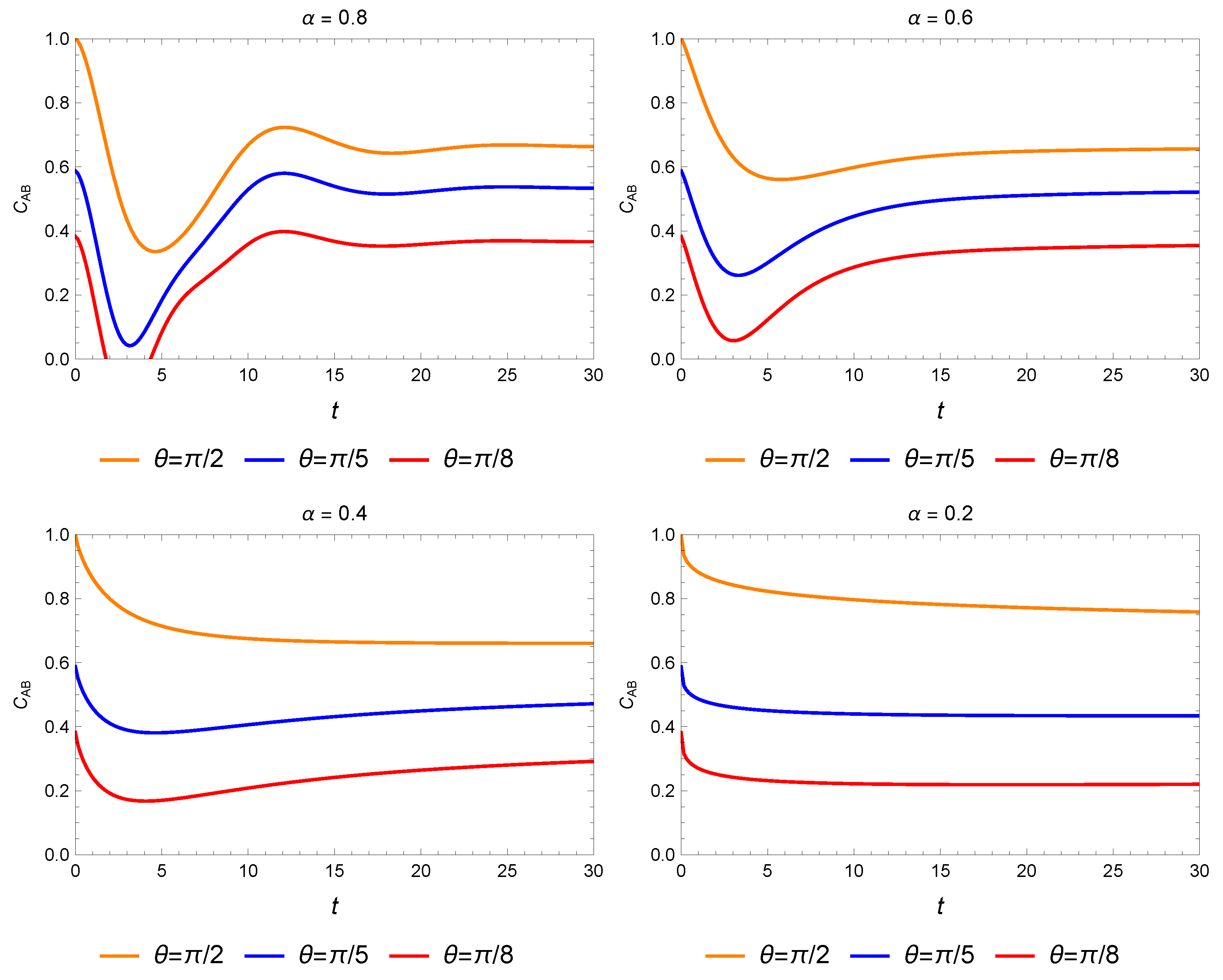
3.2. Imaginary Unit Fractional-Order Operations

This section is based on the fractional model given by Equation (2), which is characterized by raising the imaginary unit i to the fractional power $\alpha$. The model used and the corresponding calculation process are not elaborated here, we directly present the results. Considering that the shared entangled state is expressed by Equation (12), the entangled state after fractional order evolution over time can be expressed as

$${\rho }_{AB}^i={\displaystyle \frac{1}{N^i}}\left(\begin{array}{cccc}{a}^i& 0& 0& b^i\\ 0& c^i& 0& 0\\ 0& 0& c^i& 0\\ b^{i*}& 0& 0& d^i\end{array}\right)$$

(33)

where $x^i(x=a,b,c,d)$ represents the imaginary unit increased to the same power as the time coordinates and

$$\begin{array}{c}{a}^i={sin}^2{\displaystyle \frac{\theta }{2}}+{\displaystyle \frac{1}{16}}{cos}^2{\displaystyle \frac{\theta }{2}}{\left|E_{\alpha }(-2\lambda i^{-\alpha }{t}^{\alpha })+E_{\alpha }\left(2\lambda i^{-\alpha }{t}^{\alpha }\right)-2\right|}^2\hfill \\ b^i={\displaystyle \frac{1}{4}}cos{\displaystyle \frac{\theta }{2}}sin{\displaystyle \frac{\theta }{2}}[E_{\alpha }(-2\lambda i^{-\alpha }{t}^{\alpha })+E_{\alpha }\left(2\lambda i^{-\alpha }{t}^{\alpha }\right)-2]\hfill \\ c^i={\displaystyle \frac{1}{16}}{cos}^2{\displaystyle \frac{\theta }{2}}{\left|E_{\alpha }(-2\lambda i^{-\alpha }{t}^{\alpha })-E_{\alpha }\left(2\lambda i^{-\alpha }{t}^{\alpha }\right)\right|}^2\hfill \\ d^i={\displaystyle \frac{1}{16}}{cos}^2{\displaystyle \frac{\theta }{2}}{\left|E_{\alpha }(-2\lambda i^{-\alpha }{t}^{\alpha })+E_{\alpha }\left(2\lambda i^{-\alpha }{t}^{\alpha }\right)\right|}^2\hfill \\ N^i={\displaystyle \frac{1}{4}}{cos}^2{\displaystyle \frac{\theta }{2}}({\left|E_{\alpha }\left(2\lambda i^{-\alpha }{t}^{\alpha }\right)\right|}^2+{\left|E_{\alpha }(-2\lambda i^{-\alpha }{t}^{\alpha })\right|}^2+2)+{sin}^2{\displaystyle \frac{\theta }{2}}\hfill \end{array}.$$

(34)

Therefore, the concurrence is expressed by

$$C_{AB}^i={\displaystyle \frac{1}{2}}{\displaystyle \frac{4\left|cos\frac{\theta }{2}\right|\left|sin\frac{\theta }{2}\right|\left|E_{\alpha 1}^i+E_{\alpha 2}^i+2\right|-{cos}^2\frac{\theta }{2}{\left|E_{\alpha 2}^i-E_{\alpha 1}^i\right|}^2}{{cos}^2\frac{\theta }{2}({\left|E_{\alpha 1}^i\right|}^2+{\left|E_{\alpha 2}^i\right|}^2+2)+4{sin}^2\frac{\theta }{2}}},$$

(35)

where $E_{\alpha 1}^i=E_{\alpha }\left(2\lambda i^{-\alpha }{t}^{\alpha }\right), E_{\alpha 2}^i=E_{\alpha }(-2\lambda i^{-\alpha }{t}^{\alpha })$. The dense coding capacity can be expressed as

$$\begin{array}{c}{C}^i=-{\displaystyle \frac{a^i+c^i}{N^i}}{log}_2{\displaystyle \frac{a^i+c^i}{2N^i}}-{\displaystyle \frac{c^i+d^i}{N^i}}{log}_2{\displaystyle \frac{c^i+d^i}{2N^i}}+2{\displaystyle \frac{c^i}{N^i}}{log}_2{\displaystyle \frac{c^i}{N^i}}\hfill \\ +{\displaystyle \frac{a^i+d^i-{[{\left(a^i\right)}^2-2a^i{d}^i+4{\left(b^i\right)}^2+{\left(d^i\right)}^2]}^{\frac{1}{2}}}{2N^i}}{log}_2({\displaystyle \frac{a^i+d^i-{[{\left(a^i\right)}^2-2a^i{d}^i+4{\left(b^i\right)}^2+{\left(d^i\right)}^2]}^{\frac{1}{2}}}{2N^i}})\hfill \\ +{\displaystyle \frac{a^i+d^i+{[{\left(a^i\right)}^2-2a^i{d}^i+4{\left(b^i\right)}^2+{\left(d^i\right)}^2]}^{\frac{1}{2}}}{2N^i}}{log}_2({\displaystyle \frac{a^i+d^i+{[{\left(a^i\right)}^2-2a^i{d}^i+4{\left(b^i\right)}^2+{\left(d^i\right)}^2]}^{\frac{1}{2}}}{2N^i}})\hfill \end{array}.$$

(36)

Equation (1) is equivalent to Equation (2) when $\alpha =1$, and we directly study the influence of memory on entanglement. Figure 11 shows the result of the concurrence as a function of t with $\lambda =0.3$ for different $\theta$. Compared with Figure 3, it is clearly evident that the larger the memory effect, the larger the region where entanglement suddenly disappears. In other words, memory promotes the decoherence of entangled states. This result is completely opposite to the one shown in Figure 4. Furthermore, Figure 12 illustrates the influence of memory on the dense coding capacity. Compared to Figure 6, we observe that memory effects exhibit a detrimental influence. With increasing memory strength, the interval within which the dense coding capacity exceeds 1 progressively narrows as the entanglement decreases from its maximum value to zero.

Now, we investigate the time-fractional evolution of quantum dense coding using Equation (13). Similarly, we directly present the state of the entangled state after time-fractional evolution, which can be expressed as

$${\rho }_{AB}^i={\displaystyle \frac{1}{N_1^i}}\left(\begin{array}{cccc}0& 0& 0& 0\\ 0& a_1^i& b_1^i& 0\\ 0& b_1^{i*}& c_1^i& 0\\ 0& 0& 0& d_1^i\end{array}\right),$$

(37)

where

$$\begin{array}{c}{a}_1^i={\displaystyle \frac{1}{4}}{cos}^2{\displaystyle \frac{\theta }{2}}{\left|E_{\alpha }\left(\lambda i^{-\alpha }{t}^{\alpha }\right)+E_{\alpha }(-\lambda i^{-\alpha }{t}^{\alpha })\right|}^2\hfill \\ b_1^i={\displaystyle \frac{1}{4}}sin{\displaystyle \frac{\theta }{2}}cos{\displaystyle \frac{\theta }{2}}{\left|E_{\alpha }\left(\lambda i^{-\alpha }{t}^{\alpha }\right)+E_{\alpha }(-\lambda i^{-\alpha }{t}^{\alpha })\right|}^2\hfill \\ c_1^i={\displaystyle \frac{1}{4}}{sin}^2{\displaystyle \frac{\theta }{2}}{\left|E_{\alpha }\left(\lambda i^{-\alpha }{t}^{\alpha }\right)+E_{\alpha }(-\lambda i^{-\alpha }{t}^{\alpha })\right|}^2\hfill \\ d_1^i={\displaystyle \frac{1}{4}}{\left|E_{\alpha }\left(\lambda i^{-\alpha }{t}^{\alpha }\right)-E_{\alpha }(-\lambda i^{-\alpha }{t}^{\alpha })\right|}^2\hfill \\ N_1^i={\displaystyle \frac{1}{4}}({\left|E_{\alpha }(-\lambda i^{-\alpha }{t}^{\alpha })-E_{\alpha }\left(\lambda i^{-\alpha }{t}^{\alpha }\right)\right|}^2+{\left|E_{\alpha }(-\lambda i^{-\alpha }{t}^{\alpha })+E_{\alpha }\left(\lambda i^{-\alpha }{t}^{\alpha }\right)\right|}^2)\hfill \end{array}.$$

(38)

Therefore, the concurrence is expressed by

$$C_{AB}^i={\displaystyle \frac{\left|sin\theta \right|{\left|E_{\alpha }\left(\lambda i^{-\alpha }{t}^{\alpha }\right)+E_{\alpha }(-\lambda i^{-\alpha }{t}^{\alpha })\right|}^2}{{\left|E_{\alpha }\left(\lambda i^{-\alpha }{t}^{\alpha }\right)+E_{\alpha }(-\lambda i^{-\alpha }{t}^{\alpha })\right|}^2+{\left|E_{\alpha }\left(\lambda i^{-\alpha }{t}^{\alpha }\right)-E_{\alpha }(-\lambda i^{-\alpha }{t}^{\alpha })\right|}^2}}$$

(39)

The dense coding capacity can be expressed as

$$\begin{array}{c}{C}_1^i=-{\displaystyle \frac{c_1^i}{N_1^i}}{log}_2{\displaystyle \frac{c_1^i}{2N_1^i}}-{\displaystyle \frac{a_1^i+d_1^i}{N_1^i}}{log}_2{\displaystyle \frac{a_1^i+d_1^i}{2N_1^i}}+{\displaystyle \frac{d_1^i}{N_1^i}}{log}_2{\displaystyle \frac{d_1^i}{N_1^i}}\hfill \\ +{\displaystyle \frac{a_1^i+c_1^i-{[{\left(a_1^i\right)}^2-2a_1^i{c}_1^i+4{\left(b_1^i\right)}^2+{\left(c_1^i\right)}^2]}^{\frac{1}{2}}}{2N_1^i}}{log}_2({\displaystyle \frac{a_1^i+c_1^i-{[{\left(a_1^i\right)}^2-2a_1^i{c}_1^i+4{\left(b_1^i\right)}^2+{\left(c_1^i\right)}^2]}^{\frac{1}{2}}}{2N_1^i}})\hfill \\ +{\displaystyle \frac{a_1^i+c_1^i+{[{\left(a_1^i\right)}^2-2a_1^i{c}_1^i+4{\left(b_1^i\right)}^2+{\left(c_1^i\right)}^2]}^{\frac{1}{2}}}{2N_1^i}}{log}_2({\displaystyle \frac{a_1^i+c_1^i+{[{\left(a_1^i\right)}^2-2a_1^i{c}_1^i+4{\left(b_1^i\right)}^2+{\left(c_1^i\right)}^2]}^{\frac{1}{2}}}{2N_1^i}})\hfill \end{array}.$$

(40)

The behaviors of $C_{AB}^i$ as a function of the parameter t for different parameters $\theta$ are shown in Figure 13. In comparison with Figure 7, we find that when memory effects are present (i.e., $\alpha \ne 1$), the time required for the concurrence to decay from 1 to 0 becomes longer, which is consistent with the results shown in Figure 8. However, it can be clearly observed that the minimum value of the $C_{AB}^i$ is always greater than zero regardless of the time evolution. Figure 14 shows the result of the dense coding capacity as a function of the parameter t for different $\theta$. Similar to Figure 10, the increase in memory strength ensures the advantage of quantum dense coding (e.g., for $\alpha \le 2$ and $\theta =\pi /2$).

4. Conclusions

A comparative analysis of several figures reveals that the results presented in Figure 4, Figure 6, Figure 8 and Figure 10 better align with the characteristic behavior of non-Markovian dissipative quantum systems. In contrast, Figure 11, Figure 12, Figure 13 and Figure 14 exhibit trends that deviate from this physical expectation. By comparing Figure 3 with Figure 4 and Figure 11, we observe that Figure 4 suggests that increasing memory strength can effectively suppress the phenomenon of entanglement sudden death, slowing the decay of entanglement and increasing its minimum value. This behavior is consistent with the role of memory in mitigating decoherence, whereas Figure 11 reveals that stronger memory effects expand the region where entanglement vanishes, implying an enhanced decoherence effect. This outcome contradicts the widely accepted understanding that memory effects typically assist in preserving quantum coherence. Similarly, Figure 6 shows that memory effects significantly improve the dense coding capacity, particularly for $\alpha \le 0.4$ and $\theta =\pi /2$, enabling the capacity to remain above 1 for extended periods. Conversely, Figure 12 illustrates a detrimental impact: the interval during which the capacity exceeds 1 shrinks as memory increases. This is inconsistent with the commonly accepted view that memory effects prolong quantum advantage in noisy environments. The comparison between Figure 8 and Figure 13 further supports this conclusion. By comparing Figure 7 with Figure 8 and Figure 13, it is observed that the presence of memory effects (i.e., $\alpha \ne 1$) increases the time required for entanglement to decay from its maximum to minimum, indicating a slowing down of information loss. However, Figure 13 does not show a complete disappearance of entanglement. This absence of complete decoherence diverges from typical dissipative system behavior, thereby reinforcing the relevance of Figure 8. Lastly, Figure 10 highlights how memory effects delay the decay of dense coding capacity and extend the duration during which it remains above 1, again supporting the positive role of memory. Although Figure 14 shows a similar advantage, the parameter conditions under which it occurs are not entirely consistent with realistic dissipative settings, making the result less representative.

In summary, we systematically investigated the memory effects introduced by the time-fractional Schrödinger equation proposed by Naber on quantum entanglement and dense coding capacity under amplitude damping noise. By conducting numerical analyses of the system’s dynamical behavior, we compare two formulations of the time-fractional model: one where the imaginary unit is subjected to fractional operations, and another where it is not. The results suggest that the formulation without fractional operations on the imaginary unit (Equation (1)) may be more suitable for describing non-Markovian (power-law) behavior in dissipative environments. This finding provides a more physically meaningful interpretation of the memory effects in time-fractional quantum dynamics. Considering the characteristics of dissipative systems, this finding also responds to fundamental concerns regarding the violation of unitarity and the lack of probability conservation in the time-fractional Schrödinger equation. We hope that our study provides a new perspective for the application of fractional quantum mechanics in realistic open quantum systems and offers theoretical support for modeling phenomena such as decoherence and information degradation.

We should finally mention that in this work, the time-fractional Schrödinger equation is treated as a phenomenological model for describing non-Markovian effects. Its effectiveness stems from the mathematical capacity of fractional derivatives to represent memory, rather than from a modification of the fundamental principles of quantum mechanics. Although the fractional order $\alpha$ in TFSE allows for the tuning of memory strength, its quantitative correspondence to real physical systems remains to be established through microscopic derivations. Therefore, a key direction of our future research will focus on developing microscopic foundations and experimental verification of the TFSE framework. In terms of microscopic derivation, the theoretical construction of fractional models should be grounded in the first principles of quantum mechanics. Most existing formulations of the time-fractional Schrödinger equation are still phenomenological extensions, lacking a direct mapping to concrete microscopic mechanisms. It is therefore essential to investigate whether fractional dynamics can emerge naturally from the fundamental evolution of open quantum systems under specific coupling structures, spectral densities, or time-delay mechanisms. On the experimental validation side, efforts should focus on establishing a quantitative correspondence between the fractional order parameter $\alpha$ and microscopic environmental features—such as the spectral density function of a structured reservoir or the coupling configuration in quantum simulators. Realizing such a parameter-structure mapping would be a crucial step toward transforming fractional models from purely mathematical constructs into physically implementable theories. This would significantly help to bridge the gap between phenomenological modeling of the time-fractional Schrödinger equation and experimentally controllable non-Markovian quantum dynamics.

References

1. Einstein, A.; Infeld, L. Evolution of Physics; Simon and Schuster: New York, NY, USA, 1966. [Google Scholar]
2. Feynman, R.P.; Hibbs, A.R.; Styer, D.F. Quantum Mechanics and Path Integrals; Courier Corporation: North Chelmsford, MA, USA, 2010. [Google Scholar]
3. Sakurai, J.J.; Napolitano, J. Modern Quantum Mechanics; Cambridge University Press: Cambridge, UK, 2020. [Google Scholar]
4. Man, Z.X.; Xia, Y.J.; Lo, F.R. Harnessing non-Markovian quantum memory by environmental coupling. Phys. Rev. A 2015, 92, 012315. [Google Scholar] [CrossRef]
5. Goswami, K.; Giarmatzi, C.; Monterola, C.; Shrapnel, S.; Romero, J.; Costa, F. Experimental characterization of a non-Markovian quantum process. Phys. Rev. A 2021, 104, 022432. [Google Scholar] [CrossRef]
6. Abu-Nada, A.; Banerjee, S.; Sabale, V.B. Exploring the non-Markovian dynamics in depolarizing maps. Phys. Rev. A 2024, 110, 052209. [Google Scholar] [CrossRef]
7. Wyss, W. The fractional diffusion equation. J. Math. Phys. 1986, 27, 2782–2785. [Google Scholar] [CrossRef]
8. Laskin, N. Fractional Schrödinger Equation. Phys. Rev. E 2002, 66, 056108. [Google Scholar] [CrossRef]
9. Micolta-Riascos, B.; Droguett, B.; Mattar Marriaga, G.; Leon, G.; Paliathanasis, A.; del Campo, L.; Leyva, Y. Fractional Time-Delayed Differential Equations: Applications in Cosmological Studies. Fractal Fract. 2025, 9, 318. [Google Scholar] [CrossRef]
10. Haque, R.; Rahaman, M.; Alrasheedi, A.F.; Chalishajar, D.; Mondal, S.P. Fractional Calculus for Neutrosophic-Valued Functions and Its Application in an Inventory Lot-Sizing Problem. Fractal Fract. 2025, 9, 433. [Google Scholar] [CrossRef]
11. Naber, M. Time fractional Schrödinger equation. J. Math. Phys. 2004, 45, 3339. [Google Scholar] [CrossRef]
12. Wei, D.M.; Liu, H.L.; Li, Y.M.; Wan, L.; Qin, S.; Wen, Q.; Gao, F. Non-Markovian dynamics of time-fractional open quantum systems. Chaos Solitons Fractals 2024, 182, 114816. [Google Scholar] [CrossRef]
13. Zu, C.J.; Yu, X.Y. Memory effect in time fractional Schrödinger equation. Chin. Phys. B 2024, 33, 020501. [Google Scholar] [CrossRef]
14. Zu, C.J.; Yu, X.Y. The time-fractional Schrödinger equation in the context of non-Markovian dynamics with dissipation. J. Chem. Phys. 2025, 162, 074310. [Google Scholar] [CrossRef] [PubMed]
15. Lu, L.Z.; Yu, X.Y. Time fractional evolution of the two-level system interacting with light field. Laser Phys. Lett. 2017, 14, 115202. [Google Scholar] [CrossRef]
16. Wang, G.W.; Xu, T.Z. Optical soliton of time fractional Schrödinger equations with He’s semi-inverse method. Laser Phys. 2015, 25, 055402. [Google Scholar] [CrossRef]
17. Zu, C.J.; Gao, Y.M.; Yu, X.Y. Time fractional evolution of a single quantum state and entangled state. Chaos Solitons Fractals 2021, 147, 110930. [Google Scholar] [CrossRef]
18. Zu, C.J.; Yu, X.Y. Time fractional Schrödinger equation with a limit based fractional derivative. Chaos Solitons Fractals 2022, 57, 111941. [Google Scholar] [CrossRef]
19. Wei, D.M.; Liu, H.L.; Li, Y.M.; Gao, F.; Qin, S.J.; Wen, Q.Y. Quantum speed limit for Time-Fractional open systems. Chaos Solitons Fractals 2023, 175, 114065. [Google Scholar] [CrossRef]
20. Allati, A.E.; Bukbech, S.; Anouz, K.E.; Allali, Z.E. Entanglement versus Bell non-locality via solving the fractional Schrödinger equation using the twisting model. Chaos Solitons Fractals 2024, 179, 114446. [Google Scholar] [CrossRef]
21. Sayer, T.; Montoya-Castillo, A. Compact and complete description of non-Markovian dynamics. J. Chem. Phys. 2023, 158, 014105. [Google Scholar] [CrossRef]
22. Li, Z.Y.; Shen, H.Z. Non-Markovian dynamics with a giant atom coupled to a semi-infinite photonic waveguide. Phys. Rev. A 2024, 109, 023712. [Google Scholar] [CrossRef]
23. Pandey, D.; Wubs, M. Collective photon emission in solid state environments: Concatenating non-markovian and markovian dynamics. Phys. Rev. Res. 2024, 6, 033044. [Google Scholar] [CrossRef]
24. Gribben, D.; Rouse, D.M.; Iles-Smith, J.; Strathearn, A.; Maguire, H.; Kirton, P.; Nazir, A.; Gauger, E.M.; Lovett, B.W. Exact dynamics of nonadditive environments in non-Markovian open quantum systems. PRX Quantum 2022, 3, 010321. [Google Scholar] [CrossRef]
25. Milz, S.; Modi, K. Quantum stochastic processes and quantum non-Markovian phenomena. PRX Quantum 2021, 2, 030201. [Google Scholar] [CrossRef]
26. Lu, L.Z.; Yu, X.Y. The fractional dynamics of quantum systems. Ann. Phys. 2018, 392, 260–271. [Google Scholar] [CrossRef]
27. Iomin, A. Fractional-time quantum dynamics. Phys. Rev. E 2009, 80, 022103. [Google Scholar] [CrossRef] [PubMed]
28. Saxena, R.K.; Saxena, R.; Kalla, S.L. Computational solution of a fractional generalization of the Schrödinger equation occurring in quantum mechanics. Appl. Math. Comput. 2010, 216, 1412–1417. [Google Scholar] [CrossRef]
29. Odibat, Z.M. Analytic study on linear systems of fractional differential equations. Comp. Math. Appl. 2010, 59, 1171–1183. [Google Scholar] [CrossRef]
30. Wootters, W.K. Entanglement of Formation of an Arbitrary State of Two Qubits. Phys. Rev. Lett. 1997, 80, 2245. [Google Scholar] [CrossRef]
Figure 1. The sketch map of quantum dense coding under amplitude damping noise.
Fractalfract 09 00501 g001
Figure 2. The schematic diagram of the double J-C model.
Fractalfract 09 00501 g002
Figure 3. The concurrence C A B as a function of t with λ = 0.3 ,   α = 1 .
Fractalfract 09 00501 g003
Figure 4. The concurrence C A B as a function of t with λ = 0.3 for different θ and α .
Fractalfract 09 00501 g004
Figure 5. The dense coding capacity C as a function of t with λ = 0.3 ,   α = 1 for different θ .
Fractalfract 09 00501 g005
Figure 6. The dense coding capacity C as a function of t with λ = 0.3 for different θ and α .
Fractalfract 09 00501 g006
Figure 7. The C A B as a function of t with λ = 0.3 ,   α = 1 for different θ .
Fractalfract 09 00501 g007
Figure 8. The C A B as a function of t with λ = 0.3 for different θ and α .
Fractalfract 09 00501 g008
Figure 9. The dense coding capacity C 1 as a function of t with λ = 0.3 ,   α = 1 for different θ .
Fractalfract 09 00501 g009
Figure 10. The dense coding capacity C 1 as a function of t with λ = 0.3 for different θ and α .
Fractalfract 09 00501 g010
Figure 11. The C A B i as a function of t with λ = 0.3 for different θ .
Fractalfract 09 00501 g011
Figure 12. The dense coding capacity C i as a function of t with λ = 0.3 for different θ and α .
Fractalfract 09 00501 g012
Figure 13. The C A B i as a function of t with λ = 0.3 for different θ .
Fractalfract 09 00501 g013
Figure 14. The dense coding capacity C 1 i as a function of t with λ = 0.3 for different θ and α .
Fractalfract 09 00501 g014
Disclaimer/Publisher’s Note: The statements, opinions and data contained in all publications are solely those of the individual author(s) and contributor(s) and not of MDPI and/or the editor(s). MDPI and/or the editor(s) disclaim responsibility for any injury to people or property resulting from any ideas, methods, instructions or products referred to in the content.